Please cite this article as: S. Poursafary, N. Javadian, R. Tavakkoli-Moghaddam, Seeker Evolutionary Algorithm (SEA): a Novel Algorithm for Continuous Optimization, International Journal of Engineering (IJE), TRANSACTIONS A: Basics Vol. 27, No. 10, (October 2014) 1601-1610
International Journal of Engineering
J o u r n a l H o m e p a g e : w w w . i j e . i rSeeker Evolutionary Algorithm (SEA): a Novel Algorithm for Continuous
Optimization
S. Poursafary a,*, N. Javadiana, R. Tavakkoli-Moghaddamb,c
a Department of Industrial Engineering, Mazandaran University of Science & Technology, Babol, Iran b School of Industrial Engineering, College of Engineering, University of Tehran, Tehran, Iran c Research Center for Organizational Processes Improvement, Sari, Iran
P A P E R I N F O
Paper history: Received 19 April 2013
Received in revised form 20 June 2014 Accepted 26 June 2014
Keywords:
Evolutionary Algorithms Meta-heuristic Algorithms Global Optimization
Seeker Evolutionary Algorithm Multiple Global Minima
A B S T R A C T
Nowadays, in majority of academic contexts, it has been tried to consider the highest possible level of similarities to the real world. Hence, most of the problems have complicated structures. Traditional methods for solving almost all of the mathematical and optimization problems are inefficient. As a result, meta-heuristic algorithms have been employed increasingly during recent years. In this study, a new algorithm, namely Seeker Evolutionary Algorithm (SEA), is introduced for solving continuous mathematical problems, which is based on a group seeking logic. In this logic, the seeking region and the seekers located inside are divided into several sections and they seek in that special area. In order to assess the performance of this algorithm, from the available samples in papers, the most visited algorithms have been employed. The obtained results show the advantage of the proposed SEA in comparison to these algorithms. At the end, a mathematical problem is designed, which is unlike the structure of meta-heuristic algorithms. All the prominent algorithms are applied to solve this problem, and none of them is able to solve.
doi: 10.5829/idosi.ije.2014.27.10a.14
1. INTRODUCTION1
The aim of optimization is to find the best acceptable solution by considering the constraints and requirements of the problem. From this perspective, optimization is an important and determinant action. It is likely that there would be different solutions for a problem. In this case, an objective function is defined in order to compare the solutions and select the optimal solution. Many of the optimization problems are more complex and difficult to be solved by traditional optimization methods (e.g., mathematical planning method). Among the existing solutions to face these kinds of problems, the evolutionary algorithms can be applied. These algorithms give more favourable solutions in much less time in comparison to mathematical methods. However, these methods do not guarantee to provide the optimal solution. In fact, the
1*Corresponding Author’s Email: [email protected] (S.
Poursafary)
precision of solution differs depending on the spent time for calculation. In recent years, one of the most important and promising studies was “the meta-heuristic methods adopted from the nature”. These methods have some similarities with social systems or the nature. Their structures have been obtained from the evolutionary trend in the system that has had good results in solving the problems with complicated structures. In most of these types of algorithms, the seeking operation is started by producing a random population in the seeking region. Afterward, the solutions will be moved using computational intelligence available in the algorithm. This shift is performed in such a way that, after passing some steps, the population will be converged to the optimal point. The main difference of evolutionary algorithms is laid in the way that the population is moved. Up to now, various evolutionary algorithms have been introduced. A genetic algorithm (GA) is based on the evolutionary trend in the subjects of genes and propagation [1, 2].
The real-valued genetic algorithm (RGA) difference with a genetic algorithm is on the
chromosome coding, based on real numbers [3]. Simulated annealing (SA) is based on the cooling procedure of melting metals in the science of metallurgy [4]. Ant colony optimization (ACO) is based on utilizing pheromones by ants to find the shortest path [5]. Particle swarm optimization (PSO) is based on mass movements of animals specially birds. In this algorithm, each solution represents as a particle in the real world. In each iteration, a particle has got a movement. The current position, previous speed, best position of particle and the best position of all particles are the factors that effect on how the particles move [6, 7]. An imperialist competitive algorithm (ICA) has been developed based on social and political strategies of the countries [8]. The gravitational search algorithm (GSA) is based on the law of gravity, in this algorithm each solution represent a planet [9]. The artificial bee colony algorithm (ABC) is based on the bee’s behaviour on foraging. In this algorithm each solution represents as a food source. In this algorithm bees are divided to: employed, onlooker and scout [10]. The bees algorithm (BA) difference with the ABC is the bees movement [11]. The BA was improved by using a shrinking process [12].
Harmony search (HS) based on the harmony in musicians notes. In this algorithm each solution represents as a musical note [13]. Cuckoo search (CS) is a new algorithm, which is based on a cuckoo bird migration [14]. The firefly algorithm (FA) structure is formed according to the mechanism of firefly light absorption (LFA) [15], which is the extended version of this algorithm that uses Lévy flights for searching feasible solution [16]. The bat algorithm (BA) is based on the echolocation in bats life [17]. The cuckoo optimization algorithm (COA) has been inspired from the cuckoo flyblow [18]. The electromagnetism-like algorithm (EM) applies a type of attraction and repulsion mechanism for charged particles [19].
Tavakkoli-Moghaddam [20] presented new
mathematical model for a p-hub location-allocation problem and proposed three meta-heuristics, namely genetic algorithm, particle swarm optimization, and simulated annealing.
In section 2, we introduce the SEA. In section 3, the performance of the SEA is shown for different problems and some comparisons will be made several algorithms.
2. SEEKER EVOLUTIONARY ALGORITHM
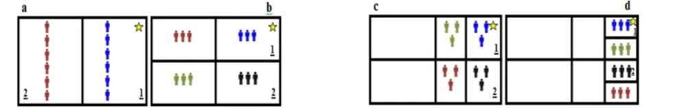
This section introduces the seeker evolutionary algorithm (SEA), which is an algorithm based on a simple seeking logic. Assume that some people want to seek their objectives in a region, which is the feasible solution space. In order to perform an optimized seeking and avoid parallelism, seekers are segmented
into some groups. They divide the seeking area into several sections and each of the groups moves to a section and starts seeking inside there. After analyzing the obtained results, the best area will be identified. In the next stage, the seeking team will divide the chosen area into some smaller sections and then, every group goes to a region and starts seeking in there. This trend will continue until the stop condition is met, which can be fulfilling some extents of the objective or the time, or having no significant evolutionary improvement in the seeking procedure. It can be expressed that in all continuous meta-heuristic algorithms we are facing with similar types of motion trends. The solutions move towards the area, which has had a good fitness up to now. However, it is with a difference, which in the movement is made based on a phenomenon in the nature.
Figure 1. Seekers’ motion trend in the solution area
This structure leads to a balanced trend towards a convergence to the optimal solution. In many of the algorithms, the convergence speed of solutions is considerably high that leads to some problems for algorithms to move towards the optimal solution. The gained results from various problems show that the chosen areas are not necessarily positioned beside the best chosen area. This has accidentally happened that the chosen area 2 is always close to the chosen area 1 in this figure and this happening does not essentially occur for the entire samples.
The SEA has a main and a subsidiary loop. The main loop involves selecting the chosen areas, dividing them, and allocating the seekers into each area. The subsidiary loop involves movement of the seeker team in the area that has been specified for it. Some of the parameters used in this algorithm are as follows:
Number of the chosen areas. 0
nc :
Number of the obtained areas from dividing the chosen area.
0
na :
These two parameters should be adjusted for different problems. Usually the value 2 is suitable for them. By increasing the value of these two parameters, the possibility of missing the area, the one that the optimal value exists in there, will be diminished knowingly.
Moreover, the convergence speed of the solutions will decrease. In addition, the number of times for evaluating the objective function increases and naturally, the solving time will be both increased accordingly. When these two parameters decrease, the opposite will occur.
The minimum number of iterations to perform restart.
g
:The minimum improvement level for the objective function to perform restart.
b :
These two parameters are for restart conditions. For instance, if we consider g =5 and b=0.001, it means that in the iterations with the multiple value of 5, if the improvement of algorithm is less than 0.001, the “restart” task will be performed. “b “ can be considered in a way that after each restart, its amount decreases. This operation leads to an increase in the convergence speed of the algorithm towards the optimal point. In some problems, the existence of “restart” may cause an improvement in the algorithm performance and in others, its absence will lead to a better result. In this case, the value of “
g
“ will be adjusted equal to the maximum number of iterations or more than that.The minimum size of an area that can be divided into smaller sections.
a :
If the size of the chosen area is very small and in other words, it is less than “
a
“, we can ignore the division of this area into smaller sections. In fact, in small sizes, the algorithm can reach desirable results even without being divided. This leads to a decrease in the solving time and optimization of the algorithm structure.Number of variables that will be crushed. nv :
In order to divide the chosen areas, the value of some variables should be divided. The criterion for choosing variables is based on the distance between their upper and lower bounds, and its number is equal to nv. The obtained results from different examples show that the most desirable value for this parameter is equal to 1 or, half of or all of the number of variables. In most of the optimization problems, considering all the limitations, the value 1 is appropriate for this parameter.
One of the stop conditions for the main and subsidiary loops of the algorithm is the specific number of iterations. In this algorithm, the maximum number of the total iterations of the algorithm is equal to maxiter0 * maxiter1 *na0 * nc0. The seekers’ motion in their seeking area (i.e., the subsidiary loop of the algorithm) is performed by:
(1) 1
1
2
( )
( (0,1) ( )
new old
old w
w Ran
Seeker Seeker
Best Seeker Seeker d
=
´
-´ +
´
maxiter0: The maximum number of iterations of the main loop.
Figure 2. Seekers’ movement towards the best seeker
In fact, each seeker in each stage moves towards.
The best seeker is in its group and there is a deviation in its movement path. The creation of this deviation is obtained from multiplying random numbers (equals to the number of variables) to the seeker’s distance from the best seeker. The trend of this movement is shown in Figure 2. In fact, if the values of W1 and W2 are considered equal to 1, the seeker is positioned between the seeker’s old position and the best seeker’s position with a little deviation. The movement of seekers based on this formula leads to their convergence to the best obtained solution.
The gained results from different examples show that the most favourable value for w1 and w2 is from 0.5 to 2. There may be some other suitable values for some problems that can be obtained from adjusting the parameter. The seeker’s motion, which is based on formula 1, leads to a situation where in some cases, the new position of the seeker in some variables might be out of the acceptable area for that variable. In these cases, the new position for those variables is located on the boundary of the acceptable area. If this occurs for the entire variables, it means that the new position of the seeker is totally out of the acceptable area. In this case, if the new position is equal to the Varmin of the given area (i.e., the lower bound of the considered area), formula 2 will be used. If the new position equals to the Varmax of the given area (i.e., the upper bound of the considered area), formula 3 will be used.
(2) Seeker new =Varmin + Rand(0.75, 1)´ (Best
Seeker1– Varmin).
(3) Seeker new =Varmax - Rand(0.75,1)´ (Varmax –
Best Seeker1 ).
According to these two formulas, when each of these seekers is completely out of the solution area, they will be positioned close to the best seeker. The values of W1 and W2 should be selected in a way that the times that the seekers are totally out of the acceptable area will be very few. The less this value is, the more desirable the obtained results well be. The results show
that the maximum number of times that this event happens should not be more than 25% of the entire cases. In the subsidiary loop of the algorithm, for the seekers that their performance value has been unsuitable, we consider another chance to improve their performance. For this purpose, we should firstly normalize the performance values of the seekers. This action is performed based on formulas 4 and 5 for
minimization and maximization functions,
respectively.
(4)
| ( ) min( ) |
( )
| max( ) min( ) |
fitness i fitness
i
fitness fitness
s =
-(5)
| max( ) ( ) |
( )
| max( ) min( ) |
fitness fitness i i
fitness fitness
s =
-If the normalized value for a seeker’s performance is less than our random number between 0 and 1, that seeker will have another chance to improve the value of its performance by another movement according to formula 1. If the seeker’s performance value improves after making this movement, the position and performance of the seeker will be updated. Obviously, the maximum number of times that this event will happen should be equal to maximum 25% of the number of the seekers in each stage.
Main Loop
Determining the feasible solution space as the chosen area.
Step 1 :
Dividing the chosen area into na0 sections.
Step 2 :
Allocating the seekers into the areas and performing the seeking operation in the subsidiary loop.
Step 3 :
Selecting nc0 premier areas as the chosen areas.
Step 4 :
If the restart condition is met, go to step 1.
Step 5 :
If the stopping condition is met, stop; otherwise, go to step 2.
Step 6 :
Figure 3. Pseudo code for the main loop SEA.
Subsidiary Loop
Producing random seekers (solutions) and calculating the fitness of each one.
Step 1 :
If a seeker’s performance is better than Best fitness1, Best
Seeker1 and Best Seeker1 will be updated.
Step 2 :
Shifting each seeker based on formula 1 and calculating its performance.
Step 3 :
Repeat Step 2
Step 4 :
Normalizing the solutions performance.
Step 5 :
If rand<s( )i : giving another chance to the seeker (i) to improve its performance
Step 6 :
if the stopping condition is met, stop; otherwise, go to step 3
Step 7:
if Best fitness1 better than Best fitness0 update Best
fitness0 and Best Seeker0
Step 8:
Figure 4. Pseudo code for the subsidiary loop SEA
Best Seeker0 : The best solution found in the entire algorithm.
The pseudo-codes for the SEA’s main and subsidiary loops are shown in Figures 3 and 4, respectively. The most important and main ideas are to divide the search space. This procedure avoids unnecessary and repetitive searches a lot. In most algorithms, an evolutionary process searches a search space region many times and useless. This algorithm is based on regular and objectively searches. The movement searchers is similar to the movement solutions in the ICA and PSO algorithms, of course the unique feature of this algorithm is dividing the search space.
3. VALIDATION OF THE SEA
In this section, in order to validate the performance of the proposed algorithm, 11 benchmark functions are used. The information about this problem is presented in Section 3.1. In Section 3.2, some problems are utilized to present the efficiency of SEA. In Section 3.3, a comparison is made between the performance of the SEA, CICA3, ICA and OICA. This action is repeated for the RGA, GSA and PSO algorithms in Section 3.4, and ABS, IBA and HS algorithms in Section 3.5, and FA, CS, BA and LFA algorithms in Section 3.6. In these sections, the numbers in the tables are in this format: 80± 10(100%); which shows the average of 80, the standard deviation of 10, and the success rate of 100%. In Section 3.7, the disability of meta-heuristic algorithms in obtaining an optimal solution in some continuous optimization problems has been discussed by presenting an example.
3. 1.Benchmark Functions In order to assess the performance of the SEA, several benchmark functions are used that the information about tens of them is presented in the beginning of this section and in Table 1 [21]. In this table, d is the dimension of the function. All the functions are of the minimization type and the most optimal value for these functions is the least one. The optimal solution for each function has been also mentioned in this table.
3. 2. Performance of the SEA In order to display the motion trend of the seekers in iterations of the SEA and the efficiency of the algorithm, the function F1 is used. Function F1:
0
sin(4 ) 1.1 sin(2 )
0 10, 10,
minimum : (9.039,8.668) 18.5547
f x
f y
x y y
x < <
= ´ + ´
< <
=
-(6)
For this function, the number of seekers is set to 20. Moreover, nc0=1, na0=2, maxiter1=10, nv=1, a b= =0 and the value for
g
is set to 50 in this case. Actually, the “restart” action is not performed for this function.The parameters of the algorithm show that one chosen area is selected and divided into two parts in each stage. The division task is obtained from crushing the space of a selected variable. The variable that has the widest domain will be crushed. The seeking operation in each crushed area is performed in 10 iterations and with 10 seekers.
3. 3. A Comparison with ICA, OICA and CICA3 In order to introduce and evaluate the performance of the proposed algorithm, The existing problems in Table 1 are used, in which the dimension of problems is as 10, the number of a population is as 30, and the maximum times of iteration is as 2000. The number of executions to evaluate and compare the performance of their considered algorithms is assumed as 100. The information in Table 2 for the algorithms CICA3, OICA and ICA is obtained from the same study.
In this study, those four problems with the dimension of 10 are used to compare the performance of our proposed algorithm. The number of a population for the SEA is assumed as 30, the maximum number of iterations is as 2000, and a b= =0. The average results from 100 times of the algorithm in addition to the parameters’ values for SEA are mentioned in Table 2. The results show that the SEA has a better performance in comparison with other three algorithms on an equal basis.
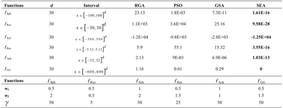
3. 4. A Comparison with RGA, PSO and GSA
Rashedi et al. [9] used 23 benchmark functions in their research in order to introduce and evaluate the performance of the GSA algorithm. Among these problems, six problems that are also among the problems in this study are selected. They set the number of population and maximum number of iterations equal to 50 and 1000, respectively. The average results from execution of the algorithms PSO, RGA and GSA for 30 times are demonstrated in Table 3. For SEA, the number of population is considered as 40 and maximum times of iterations as 1000. For this function, Rosenbrock nc0=1, na0=8, maxiter0=25,
maxiter1=5, a b= =0, nv=d and for the other functions, we have na0=2, maxiter0=50, nv=d,
maxiter1=5, a b= =0, nc0=2. The average of the obtained results from 30 times execution of SEA is provided in Table 3.
TABEL 1. Benchmark functions
Function name Function Global minimum
Rosenbrock 1 2 2 2
( ) (100( 1 ) ( 1) )
1
d
f x xi xi xi i
-å
= + - +
-= f(1)=0
r
Sphere ( ) 2 1 d f x xi
iå
=
= f(0)=0
r
Schwefel
( ) s in ( )
1
d
f x xi xi
iå
=
-= f(420.9687)= -418.9829d
uuuuuuur
Ackley 1 1
2
( ) 20 exp 0.2 exp cos(2 ) (20 )
1 1
d d
f x xi xi e
di di p
é ù é ù
ê ú ê ú
= - - å - å + +
ê = ú êë = úû
ë û f(0)=0
r
Rastrigin 2
( ) 10 10 cos(2 )
1 d
f x d xi xi
iå p
= +
-= éë ùû f(0)=0
r
Easom 2 2
( 1, 2) cos( 1) cos( 2) exp ( 1 ) ( 2 )
f x x = - x x éë-x -p - x -p ùû f( )pr = -1
Griewank 1 2
( ) cos( ) 1
1 1
4000
d
d x i
f x x i
iå iÕ i
= - +
= =
f(0)r =0
TABLE 2. Results obtained for the ICA, OICA, CICA3 and SEA and information about some the SEA parameters
Functions d Interval ICA OICA CICA3 SEA
f Gri 10 xÎ -[ 1 5 0 , 1 5 0]d 1.03E-10± 8.14E-10 2.36E-12± 1.21E-11 3.47E-14± 5.07E-15 0± 0
f Ack 10 x Î -
[
3 2 , 3 2]
d 7.11E-5± 8.20E-6 3.34E-6± 4.56E-7 1.02E-7± 1.23E-7 8.87E-14± 1.12E-14f Ros 10 xÎ -
[ ]
5, 5d 0.201± 0.362 0.0535± 0.043 0.0241± 0.021 2.77E-22± 1.49E-21f Ras 10 xÎ -
[
10, 10]
d 1.66E-06± 9.12E-06 1.27E-06± 7.00E-06 9.34E-09± 3.42E-08 7.10E-17± 3.49E-16Functions w1 w2 maxiter0 maxiter1 nc0 na0 nv
g
f Gri 0.5 2 15 10 3 2 d 5
f Ack 1 1 50 5 2 2 d 50
f Ros 1 1 50 5 2 2 d 20
f Ras 0.5 1.5 50 5 2 2 d 20
TABLE 3. Results obtained for the RGA, PSO, GSA and SEA and information about some the SEA parameters
Functions d Interval RGA PSO GSA SEA
f Sph 30 xÎ -
[
100, 100]
d 23.13 1.8E-03 7.3E-11 1.61E-16f Ros 30
[
30, 30]
dxÎ - 1.1E+03 3.6E+04 25.16 9.58E-28
f Sch 30 x Î -[ 5 0 0 , 5 0 0]d -1.2E+04 -9.8E+03 -2.8E+03 -1.25E+04
f Ras 30 xÎ -[5 .12 , 5.1 2]d 5.9 55.1 15.32 3.55E-16
f Ack 30
[
]
32, 32 d
xÎ - 2.13 9E-03 6.9E-06 1.03E-13
f Gri 30 x Î -
[
60 0 , 6 00]
d 1.16 0.01 0.29 0Functions f Sph f Ros f Sch f Ras f Ack f Gri
w1 0.5 0.5 1 0.5 1 0.5
w2 2 0.5 2 1.5 1 1.5
TABLE 4. Results obtained for the HS, IBA, ABC and SEA and information about some the SEA parameters
Functions d Interval HS IBA ABC SEA
f Sph 50
[
]
100,100d
xÎ - 546.25± 92.69 5.39E-16± 1.07E-16 1.19E-15± 4.68E-16 3.52E-43±2.83E-44
f Ros 50
[
]
30, 30d
xÎ - 24681± 10212 630.28± 1195.67 4.33± 5.48 5.08E-06±2.74E-05
f Ras 50 xÎ -[5.12, 5.12]d 37.6± 4.87 271.62± 32.7 0.4723± 0.4923 2.48E-15±6.1E-15
f Gri 50
[
]
600, 600d
xÎ - 5.81± 0.9161 134.05± 24.14 0.5721± 0.9216 0±0
f Ack 50
[
]
32, 32d
xÎ - 5.28± 0.4025 8.43± 7.7 4.38E-8± 4.65E-8 2.66E-15±0
TABLE 5. Results obtained for the CS, FA, LFA, BA and SEA and information about some the SEA parameters
Functions ns0 w1 w2 maxiter1
g
bf Sph 20 0.5 1.5 5 100 0
f Sch 12 1 2 3 10 0
f Ack 12 1 1 3 100 0
f Eas 20 0.5 2 3 40 1
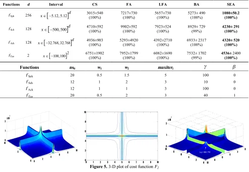
Figure 5. 3-D plot of cost function F2
Functions f Sph f Ros f Ras f Gri f Ack
w1 1 0.5 0.5 0.5 1
w2 1 0.5 1.5 2 1
g
80 10 25 100 100Functions f Sph f Ros f Ras f Gri f Ack
w1 1 0.5 0.5 0.5 1
w2 1 0.5 1.5 2 1
g
80 10 25 100 100Functions d Interval CS FA LFA BA SEA
f Sph 256 xÎ -
[
5.12, 5.12]
d 3015(100%) ±540 7217(100%) ±730 5657(100%) ±730 5273(100%) ± 490 1080(100%) ±50.2f Sch 128 xÎ -
[
500, 500]
d 4710(100%) ±592 9902(100%) ±592 7923(100%) ±524 8929(99%) ± 729 4230(100%) ± 291f Ack 128
[
32.768, 32.768]
d
xÎ - 4936(100%) ±903 5293(100%) ±4920 4392(100%) ±2710 6933(100%) ± 2317 4320(100%) ± 520
They considered food sources, d, maximum cycle number, and the maximum evaluation number equal to 20, 5, 2500, and 50000, respectively. The average results from 30 times execution of the algorithms are provided in Table 4. For the SEA, the number of populations, the maximum number of iterations, and maximum evaluation number are 20, 1600, and 40000, respectively. For all the functions, we considered maxiter1=5, a b= =0, nv=d, maxiter0=80, na0=2,
nc0=2, and just for the Rosenbrock function, b=0.01. The average results from 30 times execution of the SEA are mentioned in Table 4. The results show that the proposed SEA has a better performance in comparison to other three algorithms in this section on an equal basis.
3. 6. A Comparison with CS, FA, LFA and BA Yang and Deb [16] and Yang [17]used a number of test problems in their study in order to introduce and evaluate the BA, LFA, FA, and CS algorithms. The four functions available in Table 5 are selected from those problems for comparison in this research. The population of solutions for these algorithms is equal to 40. The numbers in Table 5 shows the times, in which the function is evaluated by each algorithm. Each algorithm stops whenever the deviation of its performance has the tolerances of
e
£
10
-5. Theresults obtained from 30 iterations of the algorithms are illustrated in Table 5. For the SEA and all the problems, a=0, nc0=2, na0=2, and nv=d. The results obtained from 30 executions of the SEA and the information about the other parameters are given in Table 5. The results show an advantage of the SEA compared to other four algorithms.
3. 7. Evolutionary Process of Meta-heuristics
Although the favourable performance of SEA has been shown in previous sections, it cannot be claimed that this algorithm has a desirable performance for the entire problems. Unlike other continuous algorithms that their structures are based on a phenomenon from around the world, the structure of SEA is based on the seeking space. In all meta-heuristic algorithms, a logic is followed. The basis of this logic is that any favourable solution leads the algorithm population with high probability to a more favourable solution which is highly likely that it is close to the same solution. In fact, meta-heuristic problems could be efficient in the problems in which around the optimal point, there are some points with desirable fitness. This trend is available in the majority of optimization problems. F2 is a sample of mathematical problems to present the weaknesses of meta-heuristic algorithms.
Function F2:
( )
6
2 6
1
10 5
5 10
d
i
i i
x f
x
-=
-=
- +
å
(7)0£xi £10 ; minimum : f
( )
5r =0As revealed for two dimensions, the point (5,5) is the optimal point of this function with the value zero for the objective function and the worst points, in terms of the objective function’s value, are around the optimal point. The objective function’s value for these points is
7
2 10´ . The results obtained from execution of this function on most of the well-known continuous algorithms show that no algorithm even with numerous iterations and with high populations can achieve the optimal value of this function. Most of the algorithms in the end identify one of the 4 points of (5, 0), (0, 5), (5, 10), and (10, 5) as the optimal point, which is very distant from the optimal point in terms of the objective function’s value. The value of the objective function for these points is 5
2 10´ . This happens because this function has been designed in contrast to the nature and structure of the meta-heuristic algorithms. The functions in which there are points with poor fitness around the optimal point, the algorithms will have difficulties to obtain the optimal point. For functions like F2, in which the worst points are located exactly around the best point, algorithms are unable to find the optimal point. If an algorithm is designed that is able to have a good performance for this problem, it will definitely have difficulties in other continuous optimization problems. It is happens because, the structure of these two problems is in contrast with each other. Therefore, the algorithm will be viable, the one which has a favourable performance for both defined continuous optimization problems. Fortunately, the number of the continuous optimization problems that has a similar structure like F2 is very few. Thus, the meta-heuristic algorithms are still accounted as the appropriate options for solving such problems.
4. CONCLUSION
condition was met, the algorithm restarted its trend from the beginning. In fact, this algorithm had been constructed based on a purposeful seeking logic. The structure of the SEA was in a way that there is a balance in the convergence of the solutions towards the optimal solution. The results obtained from the comparison of the proposed SEA with some other algorithms showed the more favourable performance of the SEA. Although various examples show the great capability of this algorithm, we are unable to claim that it has the best performance for all continuous optimization problems. In fact, this algorithm can be one of the suitable options to obtain the optimal solution for these kinds of problems.
5. REFERENCES
1. Melanie, M., "An introduction to genetic algorithms",
Cambridge, Massachusetts London, England, Fifth printing, Vol. 3, (1999).
2. Tavakkoli-Moghaddam R., Jolai F., Khodadadeghan Y. and Haghnevis M., "A mathematical model of a multi-criteria parallel machine scheduling problem: A genetic algorithm",
International Journal of Engineering, Vol. 19, No. 1, (2006), 79-86.
3. Tang, P.-H. and Tseng, M.-H., "Adaptive directed mutation for real-coded genetic algorithms", Applied Soft Computing, Vol. 13, No. 1, (2013), 600-614.
4. Kirkpatrick, S., Gelatt, C.D. and Vecchi, M.P., "Optimization by simmulated annealing", Science, Vol. 220, No. 4598, (1983), 671-680.
5. Dorigo M. and Caro G.D., "Ant colony optimization: A new meta-heuristic", in in: Proc. of the Congress on Evolutionary Computation, Washington, DC, IEEE Press, Piscataway, NJ. (1999), 1470-1477.
6. Tavakkoli-Moghaddam, R., Makui, A., Khazaei, M. and Ghodratnama, A., "Solving a new bi-objective model for a cell formation problem considering labor allocation by multi-objective particle swarm optimization", International Journal of Engineering-Transactions A: Basics, Vol. 24, No. 3, (2011), 249-255.
7. Chen, D. and Zhao, C., "Particle swarm optimization with adaptive population size and its application", Applied Soft Computing, Vol. 9, No. 1, (2009), 39-48.
8. Atashpaz-Gargari, E. and Lucas, C., "Imperialist competitive algorithm: An algorithm for optimization inspired by imperialistic competition", in Evolutionary Computation,. CEC. IEEE Congress on, IEEE. (2007), 4661-4667.
9. Rashedi, E., Nezamabadi-Pour, H. and Saryazdi, S., "Gsa: A gravitational search algorithm", Information Sciences, Vol. 179, No. 13, (2009), 2232-2248.
10. Karaboga, D. and Akay, B., "A comparative study of artificial bee colony algorithm", Applied Mathematics and Computation, Vol. 214, No. 1, (2009), 108-132.
11. Pham, D., Ghanbarzadeh, A., Koc, E., Otri, S., Rahim, S. and Zaidi, M., "The bees algorithm-a novel tool for complex optimisation problems", in Proceedings of the 2nd Virtual International Conference on Intelligent Production Machines and Systems (IPROMS). (2006), 454-459.
12. Karaboga, D. and Akay, B., "Artificial bee colony (abc), harmony search and bees algorithms on numerical optimization", in Innovative Production Machines and Systems Virtual Conference., (2009).
13. Geem, Z.W., Kim, J.H. and Loganathan, G., "A new heuristic optimization algorithm: Harmony search", Simulation, Vol. 76, No. 2, (2001), 60-68.
14. Yang, X.-S. and Deb, S., "Engineering optimisation by cuckoo search", International Journal of Mathematical Modelling and Numerical Optimisation, Vol. 1, No. 4, (2010), 330-343. 15. Yang, X.-S., Firefly algorithms for multimodal optimization, in
Stochastic algorithms: Foundations and applications., Springer. (2009). 169-178.
16. Yang, X.-S., Firefly algorithm, levy flights and global optimization, in Research and development in intelligent systems xxvi., Springer (2010). 209-218.
17. Yang, X.-S., A new metaheuristic bat-inspired algorithm, in Nature inspired cooperative strategies for optimization (nicso)., Springer, (2010). 65-74.
18. Rajabioun, R., "Cuckoo optimization algorithm", Applied Soft Computing, Vol. 11, No. 8, (2011), 5508-5518.
19. Alikhani, M.G., Javadian, N. and Tavakkoli-Moghaddam, R., "A novel hybrid approach combining electromagnetism-like method with solis and wets local search for continuous optimization problems", Journal of Global Optimization, Vol. 44, No. 2, (2009), 227-234.
20. Ghodratnama, A., Tavakkoli-Moghaddam, R. and Baboli, A., "Comparing three proposed meta-heuristics to solve a new p-hub location-allocation problem", International Journal of Engineering-Transactions C: Aspects, Vol. 26, No. 9, (2013), 1043.
Seeker Evolutionary Algorithm (SEA): a Novel Algorithm for Continuous
Optimization
S. Poursafary a, N. Javadiana, R. Tavakkoli-Moghaddamb,c
a Department of Industrial Engineering, Mazandaran University of Science & Technology, Babol, Iran b School of Industrial Engineering, College of Engineering, University of Tehran, Tehran, Iran c Research Center for Organizational Processes Improvement, Sari, Iran
P A P E R I N F O
Paper history: Received 19 April 2013
Received in revised form 20 June 2014 Accepted 26 June 2014
Keywords:
Evolutionary Algorithms Meta-heuristic Algorithms Global Optimization
Seeker Evolutionary Algorithm Multiple Global Minima.
هﺪﯿﮑﭼ ﯽﯾﺎﺠﻧآزا ﻪﮐ هزوﺮﻣا رد ﺮﺜﮐا ﻪﻨﯿﻣز يﺎﻫ ﯽﻤﻠﻋ ﯽﻌﺳ ﺮﺑ ﻦﯾا ﺖﺳا ﻪﮐ ﻦﯾﺮﺘﺸﯿﺑ ﺖﻫﺎﺒﺷ ﺎﺑ يﺎﯿﻧد ﯽﻌﻗاو رد ﻞﺋﺎﺴﻣ ظﺎﺤﻟ دﻮﺷ ، زا ﻦﯾا ور ﺮﺜﮐا ﻞﺋﺎﺴﻣ ياراد رﺎﺘﺧﺎﺳ هﺪﯿﭽﯿﭘ ﺪﻨﺘﺴﻫ . شور يﺎﻫ ﯽﺘﻨﺳ ياﺮﺑ ﻞﺣ ﺮﺜﮐا ﻞﺋﺎﺴﻣ ﯽﺿﺎﯾر و ﻪﻨﯿﻬﺑ يزﺎﺳ ﺪﻣآرﺎﮐﺎﻧ ﺪﻨﺘﺴﻫ . ﻪﺑ ﻦﯿﻤﻫ ﺖﻠﻋ هدﺎﻔﺘﺳا زا ﻢﺘﯾرﻮﮕﻟا يﺎﻫ اﺮﻓ يرﺎﮑﺘﺑا رد لﺎﺳ يﺎﻫ ﺮﯿﺧا ﺪﺷر ﻢﺸﭼ يﺮﯿﮔ ﻪﺘﺷاد ﺖﺳا . رد ﻦﯾا ﻖﯿﻘﺤﺗ ﻪﺑ ﯽﻓﺮﻌﻣ ﮏﯾ ﻢﺘﯾرﻮﮕﻟا ﺪﯾﺪﺟ ياﺮﺑ ﻞﺣ ﻞﺋﺎﺴﻣ ﯽﺿﺎﯾر ﻪﺘﺳﻮﯿﭘ ﻪﺘﺧادﺮﭘ ﺪﻫاﻮﺧ ﺪﺷ . يﺎﻨﺒﻣ ﻦﯾا ﻢﺘﯾرﻮﮕﻟا ﺮﺑ سﺎﺳا ﻖﻄﻨﻣ ﻮﺠﺘﺴﺟ ﯽﻫوﺮﮔ ﺖﺳا . رد ﻦﯾا ﻖﻄﻨﻣ ﻪﯿﺣﺎﻧ ﻮﺠﺘﺴﺟ و ﺎﻫﺮﮔﻮﺠﺘﺴﺟ ﻪﺑ ﺪﻨﭼ ﺖﻤﺴﻗ ﻢﯿﺴﻘﺗ ﯽﻣ ﺪﻧﻮﺷ و ﻪﺑ ﻮﺠﺘﺴﺟ رد نآ ﻪﯿﺣﺎﻧ ﯽﻣ ﺪﻧزادﺮﭘ . ياﺮﺑ ﺶﺠﻨﺳ دﺮﮑﻠﻤﻋ ﻦﯾا ﻢﺘﯾرﻮﮕﻟا زا لﺎﺜﻣ يﺎﻫ دﻮﺟﻮﻣ رد تﻻﺎﻘﻣ ﺮﭘ عﻮﺟر ﻦﯾﺮﺗ ﻢﺘﯾرﻮﮕﻟا ﺎﻫ هدﺎﻔﺘﺳا هﺪﺷ ﺖﺳا . ﺞﯾﺎﺘﻧ ﺖﺳﺪﺑ آ هﺪﻣ نﺎﺸﻧ هﺪﻨﻫد يﺮﺗﺮﺑ SEA ﺮﺑ ﻦﯾا ﻢﺘﯾرﻮﮕﻟا ﺎﻫ ﺖﺳا . رد ﺎﻬﺘﻧا ﺰﯿﻧ ﮏﯾ ﻪﻟﺎﺴﻣ ﯽﺿﺎﯾر ﯽﺣاﺮﻃ هﺪﺷ ﺖﺳا ﻪﮐ ﺮﺑ فﻼﺧ رﺎﺘﺧﺎﺳ ﻢﺘﯾرﻮﮕﻟا يﺎﻫ اﺮﻓ يرﺎﮑﺘﺑا ﺖﺳا . مﺎﻤﺗ ﻢﺘﯾرﻮﮕﻟا يﺎﻫ رﻮﻬﺸﻣ ياﺮﺑ ﻞﺣ ﻦﯾا ﻪﻟﺎﺴﻣ ﻪﺑ رﺎﮐ ﻪﺘﻓﺮﮔ هﺪﺷ ﺖﺳا ﯽﻟو ﭻﯿﻫ ماﺪﮐ ردﺎﻗ ﻪﺑ ﻞﺣ نآ ﯽﻤﻧ ﺪﻨﺷﺎﺑ .