https://doi.org/10.5194/gmd-12-1139-2019 © Author(s) 2019. This work is distributed under the Creative Commons Attribution 4.0 License.
The Polar Amplification Model Intercomparison Project (PAMIP)
contribution to CMIP6: investigating the causes and consequences
of polar amplification
Doug M. Smith1, James A. Screen2, Clara Deser3, Judah Cohen4, John C. Fyfe5, Javier García-Serrano6,7, Thomas Jung8,9, Vladimir Kattsov10, Daniela Matei11, Rym Msadek12, Yannick Peings13, Michael Sigmond5, Jinro Ukita14, Jin-Ho Yoon15, and Xiangdong Zhang16
1Met Office Hadley Centre, Exeter, UK
2College of Engineering, Mathematics and Physical Sciences, University of Exeter, Exeter, UK 3Climate and Global Dynamics, National Center for Atmospheric Research, Boulder, CO, USA 4Atmospheric and Environmental Research, Lexington, MA, USA
5Canadian Centre for Climate Modelling and Analysis, Environment and Climate Change Canada, Victoria,
British Columbia, Canada
6Barcelona Supercomputing Center (BSC), Barcelona, Spain 7Group of Meteorology, Universitat de Barcelona, Barcelona, Spain
8Alfred Wegener Institute, Helmholtz Centre for Polar and Marine Research, Bremerhaven, Germany 9Institute of Environmental Physics, University of Bremen, Bremen, Germany
10Voeikov Main Geophysical Observatory, Roshydromet, St. Petersburg, Russia 11Max-Planck-Institut für Meteorologie, Hamburg, Germany
12CERFACS/CNRS, UMR 5318, Toulouse, France
13Department of Earth System Science, University of California Irvine, Irvine, CA, USA 14Institute of Science and Technology, Niigata University, Niigata, Japan
15Gwangju Institute of Science and Technology, School of Earth Sciences and Environmental Engineering,
Gwangju, South Korea
16International Arctic Research Center, University of Alaska Fairbanks, Fairbanks, AK, USA
Correspondence:Doug M. Smith ([email protected]) Received: 23 March 2018 – Discussion started: 6 June 2018
Revised: 12 December 2018 – Accepted: 8 January 2019 – Published: 25 March 2019
Abstract. Polar amplification – the phenomenon where ex-ternal radiative forcing produces a larger change in surface temperature at high latitudes than the global average – is a key aspect of anthropogenic climate change, but its causes and consequences are not fully understood. The Polar Am-plification Model Intercomparison Project (PAMIP) contri-bution to the sixth Coupled Model Intercomparison Project (CMIP6; Eyring et al., 2016) seeks to improve our under-standing of this phenomenon through a coordinated set of numerical model experiments documented here. In partic-ular, PAMIP will address the following primary questions: (1) what are the relative roles of local sea ice and remote sea surface temperature changes in driving polar
forc-ing? How and why does the atmospheric response to Arctic sea ice depend on the model background state? What have been the roles of local sea ice and remote sea surface temper-ature in polar amplification, and the response to sea ice, over the recent period since 1979? How does the response to sea ice evolve on decadal and longer timescales?
A key goal of PAMIP is to determine the real-world sit-uation using imperfect climate models. Although the exper-iments proposed here form a coordinated set, we anticipate a large spread across models. However, this spread will be exploited by seeking “emergent constraints” in which model uncertainty may be reduced by using an observable quantity that physically explains the intermodel spread. In summary, PAMIP will improve our understanding of the physical pro-cesses that drive polar amplification and its global climate impacts, thereby reducing the uncertainties in future projec-tions and predicprojec-tions of climate change and variability.
1 Introduction
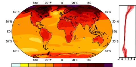
Polar amplification refers to the phenomenon in which zon-ally averaged surface temperature changes in response to cli-mate forcings are larger at high latitudes than the global aver-age. Polar amplification, especially in the Arctic, is a robust feature of global climate model simulations of recent decades (Bindoff et al., 2013) and future projections driven by anthro-pogenic emissions of carbon dioxide (Fig. 1, Collins et al., 2013). Polar amplification over both poles is also seen in sim-ulations of paleo-climate periods driven by solar or natural carbon cycle perturbations (Masson-Delmotte et al., 2013).
Observations over recent decades (Fig. 2) suggest that Arctic amplification is already occurring: recent tempera-ture trends in the Arctic are about twice the global average (Serreze et al., 2009; Screen and Simmonds, 2010; Cow-tan and Way, 2013), and Arctic sea ice extent has declined at an average rate of around 4 % decade−1 annually and more than 10 % decade−1during the summer (Vaughan et al., 2013). Climate model simulations of the Arctic are broadly consistent with the observations (Fig. 2). However, there is a large intermodel spread in temperature trends (Bind-off et al., 2013), the observed rate of sea ice loss is larger than most model simulations (Stroeve et al., 2012), and the driving mechanisms are not well understood (discussed fur-ther below). Antarctic amplification has not yet been ob-served (Fig. 2). Indeed, Antarctic sea ice extent has increased slightly over recent decades (Vaughan et al., 2013) in contrast to most model simulations (Bindoff et al., 2013), and under-standing recent trends represents a key challenge (Turner and Comiso 2017). Nevertheless, Antarctic amplification is ex-pected in the future in response to further increases in green-house gases but is likely to be delayed relative to the Arctic due to strong heat uptake in the Southern Ocean (Collins et al., 2013; Armour et al., 2016). There is mounting evidence
Figure 1. Polar amplification in projections of future climate change. Temperature change patterns are derived from 31 CMIP5
model projections driven by RCP8.5, scaled to 1◦C of global mean
surface temperature change. The patterns have been calculated by computing 20-year averages at the end of the 21st (2080–2099) and 20th (1981–2000) centuries, taking their difference and nor-malising it, grid point by grid point, by the global average tempera-ture change. Averaging across models is performed before normal-isation, as recommended by Hind et al. (2016). The colour scale
represents degrees Celsius per 1◦C of global average temperature
change. Zonal means of the geographical patterns are shown for each individual model (red) and for the multi-model ensemble mean (black).
that polar amplification will affect the global climate system by altering the atmosphere and ocean circulations, but the precise details and physical mechanisms are poorly under-stood (discussed further below).
The Polar Amplification Model Intercomparison Project (PAMIP) will investigate the causes and global consequences of polar amplification, through creation and analysis of an unprecedented set of coordinated multi-model experiments and strengthened international collaboration. The broad sci-entific objectives aim to
– provide new multi-model estimates of the global climate response to Arctic and Antarctic sea ice changes; – determine the robustness of the responses between
dif-ferent models and the physical reasons for differences; – improve our physical understanding of the mechanisms
causing polar amplification and its global impacts; and – harness increased process understanding and new
multi-model ensembles to constrain projections of future cli-mate change in the polar regions and associated global climate impacts.
Figure 2. Recent Arctic and Antarctic temperature trends
(◦C decade−1) in(a, b)observations and(c, d)model simulations.
Linear trends are shown for the 30-year period (1988 to 2017). Ob-servations are taken as the average of HadCRUT4 (Morice et al., 2012), NASA-GISS (Hansen et al., 2010) and NCDC (Karl et al., 2015). Model trends are computed as the average from 25 CMIP5 model simulations driven by historical and RCP4.5 radiative forc-ings.
1. How does the Earth system respond to forcing? This will be addressed through coordinated multi-model ex-periments to understand the causes and consequences of polar amplification.
2. What are the origins and consequences of systematic model biases? Specific experiments are proposed to in-vestigate the role of model biases in the atmospheric re-sponse to sea ice.
3. How can we assess future climate changes given climate variability, predictability and uncertainties in scenarios? Analysis of PAMIP experiments will focus on process understanding in order to constrain future projections. This paper describes the motivation for PAMIP and docu-ments the proposed model experidocu-ments and suggested analy-sis procedure. An overview of the causes and consequences of polar amplification is given in Sects. 2 and 3 before outlining the need for coordinated model experiments in Sect. 4. The proposed PAMIP experiments and analysis are documented in Sect. 5 and the data request is described in Sect. 6. Interactions with other Model Intercomparison
Projects (MIPs) are discussed in Sect. 7. A summary is pro-vided in Sect. 8, and data availability is described in Sect. 9. Details of the forcing data are given in Appendix A, and tech-nical details for running the experiments are given in Ap-pendix B.
2 Causes of polar amplification
Polar amplification arises both from the pattern of radiative forcing (Huang et al., 2017) and several feedback mecha-nisms that operate at both low and high latitudes (Taylor et al., 2013; Pithan and Mauritsen, 2014). The most well estab-lished of these is the surface albedo feedback at high latitudes (Manabe and Stouffer, 1994; Hall, 2004) in which melting of highly reflective sea ice and snow regions results in increased absorption of solar radiation which amplifies the warming. However, lapse rate and Planck feedbacks play a larger role in climate model simulations of Arctic amplification than the surface albedo feedback (Pithan and Mauritsen, 2014). Lapse rate feedback is negative at lower latitudes where the upper troposphere is heated by latent heat released by rising air parcels but becomes positive at high latitudes where the more stable atmosphere restricts local surface-driven warming to low altitudes. Hence, lapse rate feedback directly drives po-lar amplification by acting to reduce the warming at low lat-itudes and increase the warming at high latlat-itudes. Planck feedback is negative everywhere and opposes global warm-ing by emission of long-wave radiation. However, it operates more strongly at warmer lower latitudes and therefore con-tributes to polar amplification. Other feedbacks are also tentially important in controlling temperature trends in po-lar regions, including water vapour (Graversen and Wang, 2009) and clouds (Vavrus, 2004), and changes in heat trans-port in the atmosphere (Manabe and Wetherald, 1980) and ocean (Khodri et al., 2001; Holland and Bitz, 2003; Spielha-gen et al., 2011). Although some of these may operate more strongly at lower latitudes, thereby opposing polar amplifi-cation (Pithan and Mauritsen, 2014), they are important in controlling the overall temperature trends and hence the mag-nitude of polar amplification.
influ-enced by changes in atmospheric circulation (Turner et al., 2015; Raphael et al., 2015; Jones et al., 2016b), notably an increase in the Southern Annular Mode (SAM) and a deep-ening of the Amundsen Sea Low (ASL). The SAM increase, especially during austral summer, has been linked to ozone depletion (Thompson and Solomon, 2002), but its role in driving warming of the Antarctic Peninsula, which peaks in winter and spring, is unclear (Smith and Polvani, 2017). The deepening of the ASL has likely been influenced by both PDV (Purich et al., 2016; Schneider et al., 2015; Schnei-der and Deser, 2017) and AMV (Li et al., 2014). Freshen-ing of Antarctic surface waters from meltFreshen-ing ice shelves may also have influenced recent Antarctic sea ice and tempera-ture trends (Bintanja et al., 2013), though the magnitude of this effect is uncertain (Swart and Fyfe, 2013).
3 Consequences of polar amplification
Polar amplification will affect the melting of polar ice sheets and hence sea level rise, and the rate of carbon uptake in the polar regions. These impacts are investigated by the Ice Sheet Model Intercomparison Project (Nowicki et al., 2016) and the Coupled Climate–Carbon Cycle Model Intercompar-ison Project (Jones et al., 2016a), respectively. PAMIP, de-scribed here, will focus on the impacts of sea ice changes on the global climate system through changes in the atmo-sphere and ocean circulation. This is an area of intensive scientific interest and debate, as summarised in several re-cent reviews (Cohen et al., 2014; Vihma, 2014; Walsh, 2014; Barnes and Screen, 2015; Overland et al., 2015, Screen et al., 2018). A number of hypothesised consequences of a warm-ing Arctic have been proposed based on observations, in-cluding changes in the behaviour of the polar jet stream (e.g. Francis and Vavrus, 2012), that could potentially give rise to more persistent and extreme weather events. Arctic warming has also been proposed as a cause of decadal cooling trends over Eurasia (Liu et al., 2012; Mori et al., 2014; Kretschmer et al., 2017), in what has been referred to as the warm Arctic– cold continents pattern (Overland et al., 2011; Cohen et al., 2013). However, determining causality solely from observa-tions is an intractable problem. For this reason, model exper-iments with reduced sea ice have been extensively used – but to date, with little coordination between modelling groups – in an attempt to better isolate the response to sea ice loss and understand the causal mechanisms. Such experiments tend to broadly agree on the local thermodynamic response but diverge considerably on the dynamical response (e.g. Liu et al., 2012; Mori et al., 2014; Sun et al., 2016; Ogawa et al., 2018). A key area of uncertainty is the atmospheric circu-lation changes in responses to Arctic warming. By defini-tion, polar amplification will reduce the Equator-to-pole sur-face temperature gradient, potentially weakening the midlat-itude westerly winds and promoting a negative Arctic Oscil-lation (AO) or North Atlantic OscilOscil-lation (NAO). However,
this dynamic response may be opposed by a local thermody-namic low-pressure response to Arctic warming that acts to strengthen the midlatitude westerlies (Smith et al., 2017), and the overall response is unclear (Deser et al., 2015; Shepherd, 2016). Since the remote consequences of polar amplification are to a large extent governed by changes in the atmospheric circulation, it is of critical importance to attempt to constrain the circulation response to polar amplification through col-laborative modelling activities. The response to Antarctic sea ice has received far less attention. Some studies simulate an equatorward shift of the midlatitude tropospheric jet in re-sponse to reduced Antarctic sea ice (Raphael et al., 2011; Bader et al., 2013; Smith et al., 2017; England et al., 2018), but it is unclear whether this relationship will continue to hold in future as the sea ice retreats (Kidston et al., 2011). Polar amplification will also drive changes in the ocean, po-tentially giving rise to global climate impacts. For exam-ple, reduced Arctic sea ice may weaken the Atlantic merid-ional overturning circulation (Sévellec et al., 2017; Suo et al., 2017), and increased warming of the Northern Hemisphere relative to the Southern Hemisphere may shift the Intertrop-ical Convergence Zone (ITCZ) (Chiang and Bitz, 2005) af-fecting Sahel rainfall and tropical storm activity (Smith et al., 2017), and Californian drought (Cvijanovic et al., 2017). However, the extent to which the latter impacts are mitigated by changes in ocean heat transport convergence is uncertain (Tomas et al., 2016).
4 The need for coordinated model experiments
It is clear from the discussion in Sects. 2 and 3 that both the causes and consequences of polar amplification are uncer-tain. CMIP6 (Eyring et al., 2016) provides an unprecedented opportunity to improve our understanding of climate change and variability in general, and several CMIP6 MIPs will pro-vide valuable information on the causes and consequences of polar amplification in particular, as discussed in Sect. 7. PAMIP will complement the other CMIP6 MIPs by provid-ing coordinated model experiments that are specifically de-signed to investigate the physical mechanisms driving polar amplification and the climate system’s response to changes in sea ice. Improved understanding of the physical processes gained through PAMIP will enable uncertainties in future polar amplification and associated climate impacts to be re-duced.
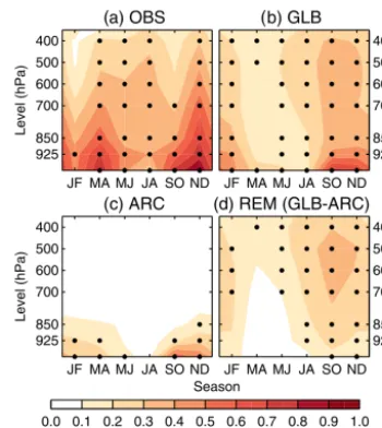
Figure 3.Local and remote drivers of Arctic warming.(a) Verti-cal and seasonal structure of the reanalysis ensemble-mean (OBS)
Arctic-mean temperature trends (1979–2008).(b–d)As in panel(a)
but for the model ensemble-mean simulations forced by observed changes in global SST and SIC (GLB), observed changes only in Arctic SIC and associated SST (ARC), and their difference (REM), respectively. Black dots show trends that are statistically significant
at the 95 % level (p <0.05). These experiments enable the relative
contributions of local (ARC) and remote (REM) processes to Arc-tic trends to be assessed, giving insight into the driving mechanisms. Source: Screen et al. (2012).
troposphere to mid-troposphere (Fig. 3a), suggesting that both local and remote processes could be important, but as-sessing their relative roles is not possible from observations alone. Model experiments in which remote sea surface tem-perature (SST) and sea ice concentration (SIC) changes are imposed separately (Kumar et al., 2010; Screen et al., 2012; Perlwitz et al., 2015) enable the contributions from local and remote processes to be quantified (Fig. 3b–d) and will be a core component of PAMIP.
It is also not possible to diagnose the climate system re-sponse to sea ice from observations alone. This is illustrated in Fig. 4, which compares the winter mean sea level response to reduced Arctic sea ice inferred from lagged regression with the simulated response obtained in model experiments driven by changes in sea ice (Smith et al., 2017). Lagged re-gression shows a pattern that projects onto a negative NAO in both the observations and in atmosphere model experiments driven by observed SIC and SST (Fig. 4a and b). These re-gressions imply a negative NAO response to reduced Arc-tic sea ice (e.g. Liu et al., 2012). However, the actual re-sponse to reduced Arctic sea ice determined from specific experiments using the same model is a weak positive NAO (Fig. 4c). This suggests that the model response (Fig. 4b) is driven by changes in SST rather than SIC. Hence, although statistical analysis can provide useful insights, the results can
Figure 4.Inability to diagnose atmospheric response to sea ice from observations alone. Linear regression between autumn (September– November) Arctic sea ice extent and winter (December–February)
mean sea level pressure (reversed sign) in (a) observations and
(b)atmosphere model experiments forced by observed SIC and SST
following the Atmosphere Model Intercomparison Project (AMIP) protocol. All time series were linearly detrended and cover the
period December 1979 to November 2009.(c) Winter mean sea
level response to reduced sea ice in atmospheric model experiments (scaled by the average autumn sea ice extent reduction). Units are
hPa per million km2. Source: Smith et al. (2017).
sometimes be misleading and need to be supported by ded-icated model experiments. However, modelling studies cur-rently simulate a full spectrum of NAO responses to reduced Arctic sea ice including negative NAO (Honda et al., 2009; Seierstad and Bader, 2009; Mori et al., 2014; Kim et al., 2014; Deser et al., 2015; Nakamura et al., 2015), positive NAO (Singarayer et al., 2006; Strey et al., 2010; Orsolini et al., 2012; Rinke et al., 2013; Cassano et al., 2014; Screen et al., 2014), little response (Screen et al., 2013; Petrie et al., 2015; Blackport and Kushner, 2016) and a response that de-pends on the details of the forcing (Alexander et al., 2004; Petoukhov and Semenov, 2010; Peings and Magnusdottir, 2014; Sun et al., 2015; Pedersen et al., 2016; Chen et al., 2016). There are many potential reasons for the different re-sponses found in modelling studies, including the following: – Differences in the magnitude of the forcing.Some stud-ies have investigated the response to sea ice perturba-tions typical of the present day and near future (e.g. Chen et al., 2016; Smith et al., 2017), while others have investigated the impact of larger changes expected to-wards the end of the century (e.g. Deser et al., 2016; Blackport and Kushner, 2016). Furthermore, interpret-ing the impact of differences in the magnitude of the forcing is particularly difficult because the relationship could be non-linear (Petoukhov and Semenov, 2010; Pe-ings and Magnusdottir, 2014; Semenov and Latif, 2015; Chen et al., 2016).
Furthermore, the responses to regional sea ice anoma-lies do not add linearly (Screen, 2017), complicating their interpretation.
– How the forcing is applied. Changes in sea ice can be imposed in different ways in coupled models, for ex-ample, by nudging the model to the required state (e.g. Smith et al., 2017; McCusker et al., 2017), or by chang-ing the fluxes of energy in order to melt some of the sea ice (e.g. Deser et al., 2016; Blackport and Kushner, 2016). The impact of these different approaches is not clear, but they could potentially contribute to the spread of results.
– Additional forcings. Isolating the response to sea ice changes can be complicated if additional forcings are imposed. For example, greenhouse-gas-induced warming of the tropical troposphere tends to increase the Equator-to-pole temperature gradient in the mid-troposphere and oppose the impact of sea ice (Deser et al., 2015; Blackport and Kushner, 2017; Oudar et al., 2017). Hence, additional steps are needed to isolate the impacts of sea ice in experiments that also include other forcings (e.g. McCusker et al., 2017).
– Different models. The response can be very sensitive to the model used. For example, Sun et al. (2015) ob-tained opposite responses in the winter polar vortex in identical forcing experiments with two different mod-els: one with a well-resolved stratosphere and one with-out. García-Serrano et al. (2017) further discuss the di-versity of potential Arctic–midlatitude linkages found in coupled models.
– Atmosphere/ocean coupling. Although many studies have used atmosphere-only models, changes in Arctic sea ice can influence SSTs surrounding the ice pack and also in remote regions, including the tropics (e.g. Deser et al., 2015; Tomas et al., 2016; Smith et al., 2017). Cou-pled models are essential to simulate these effects and may also amplify the winter midlatitude wind response to Arctic sea ice (Deser et al., 2016).
– Background state.Identical experiments with the same model but with different background states induced by different SST biases can produce opposite NAO re-sponses (Smith et al., 2017). Furthermore, rere-sponses may not be robust across experiments due to strong non-linearities in the system, which can depend on the back-ground state (Chen et al., 2016).
– Land surface. Snow cover can also influence the at-mospheric circulation (Cohen and Entekhabi, 1999; Gastineau et al., 2017), although models appear to un-derestimate the effects (Furtado et al., 2015). Differ-ences in snow cover could therefore contribute to dif-ferences in modelled responses to sea ice.
– Low signal-to-noise ratio.The atmospheric response to Arctic sea ice simulated by models is typically small compared to internal variability so that a large ensemble of simulations is required to obtain robust signals (e.g. Screen et al., 2014; Mori et al., 2014; Sun et al., 2016). Some of the different responses reported in the litera-ture could therefore arise from sampling errors. If the low signal-to-noise ratio in models is correct, then the response to Arctic sea ice could be overwhelmed by in-ternal variability (McCusker et al., 2016). However, the signal-to-noise ratio in seasonal forecasts of the NAO is too small in models (Eade et al., 2014; Scaife et al., 2014; Dunstone et al., 2016), suggesting that the mag-nitude of the simulated response to sea ice could also be too small.
PAMIP seeks to reduce these sources of differences since all simulations will follow the same experimental protocol, allowing the different model responses to be better under-stood. Additional experiments will also focus on understand-ing the roles of couplunderstand-ing, the background state and the pattern of forcing.
5 PAMIP experiments and analysis plan
Coordinated model experiments in PAMIP will address the following primary questions:
1. What are the relative roles of local sea ice and remote sea surface temperature changes in driving polar ampli-fication?
2. How does the global climate system respond to changes in Arctic and Antarctic sea ice?
Table 1.PAMIP-coordinated model experiments. The contributions of local sea ice and remote SST to polar amplification, and the response to sea ice, will be diagnosed from atmosphere-only and coupled atmosphere–ocean model experiments using different combinations of
SST and SIC representing present-day (pd), pre-industrial (pi) and future (fut, representing 2◦warming) conditions. The signals of interest
are obtained by differencing experiments, as shown in Table 2. Further details are given in Appendix B. The prefix “pa” denotes partially coupled experiments that are unique to PAMIP. We stress that the ensemble size is the minimum required and encourage groups to submit more members if possible.
Experiment Start Number Minimum
No. name Description Notes Tier year of years ensemble size
1. Atmosphere-only time slice experiments
1.1 pdSST-pdSIC Time slice forced by climatological
monthly mean SST and SIC for the
present day (pd)1,2
Present-day SST and SIC
1 2000 12 100
1.2 piSST-piSIC Time slice forced by climatological
monthly mean SST and SIC for
pre-industrial (pi) conditions3
Pre-industrial SST and SIC
2 2000 1 100
1.3 piSST-pdSIC Time slice forced by pi SST and pd
SIC3
Different SST relative to 1.1 to investigate the
1 2000 1 100
1.4 futSST-pdSIC Time slice forced by pd SIC and
fu-ture SST representing 2◦global
warming (fut)3
role of SSTs in polar
amplification 2 2000 1 100
1.5
pdSST-piArcSIC
Time slice forced by pd SST and pi
Arctic SIC3
Different Arctic SIC
relative to 1.1 to in-vestigate the impacts of present-day and future
1 2000 1 100
1.6
pdSST-futArcSIC
Time slice forced by pd SST and fut
Arctic SIC3
Arctic sea ice and the role of Arctic SIC in polar amplification
1 2000 1 100
1.7
pdSST-piAntSIC
Time slice forced by pd SST and pi
Antarctic SIC3
Different Antarctic SIC relative to 1.1 to in-vestigate the impacts of present-day and future
1 2000 1 100
1.8
pdSST-futAntSIC
Time slice forced by pd SST and fut
Antarctic SIC3
Antarctic sea ice and the role of Antarctic SIC in polar amplifica-tion
1 2000 1 100
1.9
pdSST-pdSICSIT
Time slice forced by pd sea ice thickness (SIT) in addition to SIC and SST
Investigate the impacts of sea ice thickness changes
3 2000 1 100
1.10
pdSST-futArcSICSIT
Time slice forced by pd SST and fut Arctic SIC and SIT
Investigate the impacts of sea ice thickness changes
3 2000 1 100
2. Coupled ocean–atmosphere time slice experiments
2.1 pa-pdSIC Coupled time slice constrained by
pd SIC2,4,5
2 2000 1 100
2.2 pa-piArcSIC Coupled time slice with pi Arctic
SIC3
As 1.5 and 1.6 but with coupled model
2 2000 1 100
2.3 pa-futArcSIC Coupled time slice with fut
ArcticSIC3
Table 1.Continued.
Experiment Start Number Minimum
No. name Description Notes Tier year of years ensemble size
2.4 pa-piAntSIC Coupled time slice with pi Antarctic
SIC3
As 1.7 and 1.8 but with coupled model
2 2000 1 100
2.5 pa-futAntSIC Coupled time slice with fut Antarctic
SIC3
2 2000 1 100
3. Atmosphere-only time slice experiments to investigate regional forcing
3.1
pdSST-futOkhotskSIC
Time slice forced by pd SST and fut Arctic SIC only in the Sea of Okhotsk
Investigate how the at-mospheric response
de-3 2000 1 100
3.2
pdSST-futBKSeasSIC
Time slice forced by pd SST and fut Arctic SIC only in the Barents/Kara seas
pends on the pattern of
Arctic sea ice forcing 3 2000 1 100
4. Atmosphere-only time slice experiments to investigate the role of the background state
4.1
modelSST-pdSIC
Time slice forced by pd SIC and pd SST from coupled model (2.1) rather than observations
In conjunction with ex-periments 1 and 2, iso-late the effects of the
3 2000 1 100
4.2
modelSST-futArcSIC
Time slice forced by fut Arctic SIC and pd SST from coupled model (2.1) rather than observations
background state from
the effects of coupling 3 2000 1 100
5. Atmosphere-only transient experiments
5.1
amip-climSST
Repeat CMIP6 AMIP (1979–2014) but with climatological monthly mean SST
Use CMIP6 AMIP as the control; investigate transient response,
indi-3 1979 36 3
5.2 amip-climSIC Repeat CMIP6 AMIP (1979–2014)
but with climatological monthly mean SIC
vidual years and the contributions of SST and SIC to recent climate changes
3 1979 36 3
6. Coupled ocean–atmosphere extended experiments
6.1 pa-pdSIC-ext Coupled model extended simulation
constrained with pd sea ice4,6
Experiments to investi-gate the decadal and
3 2000 100 1
6.2 pa-fut
ArcSIC-ext
Coupled model extended simulation
constrained with fut Arctic sea ice4,6
longer impacts of
Arc-tic and AntarcArc-tic sea 3 2000 100 1
6.3 pa-fut
AntSIC-ext
Coupled model extended simulation constrained with fut Antarctic sea ice4,6
ice
3 2000 100 1
each model before averaging across models, rather than cal-culating a ratio based on the multi-model-mean temperature changes (i.e. as a mean ratio, not a ratio of means).
The tier 1 experiments are atmosphere-only runs to min-imise computational costs, and lower-tier experiments inves-tigate additional aspects and provide further understanding of the physical processes. All experiments require a large en-semble to obtain robust results (Screen et al., 2014; Mori et al., 2014) and we encourage groups to submit more than the minimum requirement if they are able to. The experiments are listed in Table 1, and further technical details are given in Appendix B. Suggested combinations for diagnosing the roles of SST and sea ice in polar amplification, and the cli-mate response to sea ice, are given in Table 2. The experi-ments are grouped into six sets as follows:
1. Atmosphere-only time slice.What are the relative roles of local sea ice and remote sea surface temperature changes in driving polar amplification, and how does the global climate system respond to changes in Arctic and Antarctic sea ice? This set contains all of the tier 1 experiments and provides a multi-model assessment of the primary scientific questions addressed by PAMIP. The difference between experiments 1.1 and 1.3 pro-vides an estimate of the contribution of SST to the po-lar amplification between pre-industrial and present-day conditions. The contribution of Arctic (Antarctic) sea ice to polar amplification, as well as the atmospheric response to Arctic (Antarctic) sea ice changes between pre-industrial and present-day conditions, can be ob-tained by differencing experiments 1.1 and 1.5 (1.7). Note that the linearity of responses to SST and sea ice can be assessed by comparing with the total response diagnosed by differencing experiments 1.2 and 1.1. The contribution of Arctic (Antarctic) sea ice to future po-lar amplification, as well as the atmospheric response to Arctic (Antarctic) sea ice changes between present-day and future conditions, can be obtained by differenc-ing experiments 1.1 and 1.6 (1.8). Tier 2 experiment 1.4 provides an estimate of the contribution of SST to fu-ture polar amplification, and 1.2 provides an additional estimate of the contribution of SST to past polar am-plification. Further estimates can be obtained by differ-encing future and pre-industrial periods. Sensitivity to the magnitude of the forcing can also be investigated since differences in SST and SIC between future and pre-industrial conditions are much larger than between present-day and future or pre-industrial conditions. Tier 3 experiments 1.9 and 1.10 enable the role of Arctic sea ice thickness changes to be assessed (see Appendix B for details of sea ice thickness specification).
2. Coupled ocean–atmosphere time slice.What role does ocean–atmosphere coupling play in the response to sea ice? Previous studies have shown that such coupling
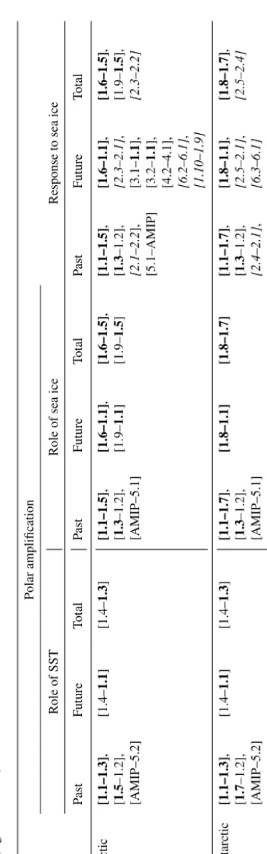
Figure 5.Arctic sea ice forcing fields. Present-day Arctic sea ice concentration for(a)September and(d)March. Differences from
present-day fields are shown for(b, e)pre-industrial and(c, f)future conditions.
potentially amplifies the response and produces addi-tional impacts in remote regions, including the tropics (Deser et al., 2015, 2016; Tomas et al., 2016; Smith et al., 2017; Oudar et al., 2017; Blackport and Kushner, 2017). Coupled model simulations are therefore needed to assess the full response to sea ice. These experiments impose the same SIC fields as used in the atmosphere-only experiments (1.1, 1.5 to 1.8; see Appendix B for further details), allowing an assessment of the role of coupling. However, it is important to note that the back-ground states are likely to be different between the cou-pled model and atmosphere-only simulations, and ex-periment set 4 is needed to isolate the effects of cou-pling (Smith et al., 2017). Experiment set 2 focusses on the short-term effects of the ocean, but the full effects will likely take longer to become established and are in-vestigated in experiment set 6.
3. Atmosphere-only time slice experiments to investigate regional forcing.How and why does the atmospheric response to Arctic sea ice depend on the regional pat-tern of sea ice forcing? Previous studies have found that the atmospheric response is potentially very sensitive to the pattern of sea ice forcing (Sun et al., 2015; Screen, 2017). This sensitivity will be investigated by speci-fying SIC changes in two different regions: the Bar-ents/Kara seas and the Sea of Okhotsk. These regions represent the Atlantic and Pacific sectors which poten-tially produce opposite responses in the stratosphere (Sun et al., 2015) and have been highlighted as impor-tant regions by several studies (e.g. Honda et al., 1996; Petoukhov and Semenov, 2010; Kim et al., 2014; Mori et al., 2014; Kug et al., 2015; Screen, 2013, 2017). 4. Atmosphere-only time slice experiments to investigate
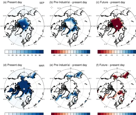
Figure 6.Arctic SST forcing fields. Present-day Arctic SST for(a)September and(d)March. Differences from present-day fields are shown for(b, e)pre-industrial and(c, f)future conditions.
on the model background state? The atmospheric re-sponse to sea ice is potentially sensitive to the model background state (Balmaseda et al., 2010; Smith et al., 2017). This is investigated in experiment set 4 by re-peating the atmosphere-only experiments (1.1 and 1.6) but specifying the climatological average SST obtained from the coupled model experiment (2.1) for the same model (as detailed in Appendix B), thereby imposing the coupled model biases. Analysis of the physical pro-cesses giving rise to sensitivity to background state could lead to an “emergent constraint” to determine the real-world situation (Smith et al., 2017), as discussed further below. Furthermore, experiment sets 1, 2 and 4 together enable the role of coupling to be isolated, as-suming the influences of coupling and background state are linear.
5. Atmosphere-only transient experiments. What have been the relative roles of SST and SIC in observed polar
amplification over the recent period since 1979? These experiments are atmosphere-only simulations of the pe-riod starting in 1979. The control is a CMIP6 DECK experiment (Eyring et al., 2016) driven by the observed time series of monthly mean SST and SIC; if necessary, the ensemble size should be increased to be the same as the PAMIP experiments. Replacing the monthly mean time series with the climatological averages for SST and SIC separately enables the impacts of transient SST and SIC to be diagnosed. Individual years of interest, and the transient response to sea ice loss, may also be inves-tigated. Note that to obtain robust results from a single model it may be necessary to provide 30 or more en-semble members (Sun et al., 2016).
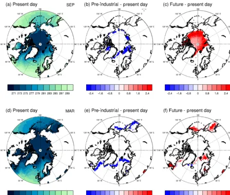
mod-Figure 7.Antarctic sea ice forcing fields. Present-day Antarctic sea ice concentration for(a)September and(d)March. Differences from
present-day fields are shown for(b, e)pre-industrial and(c, f)future conditions.
ulated by decadal and longer-timescales changes in the ocean (Tomas et al., 2016; Sévellec et al., 2017). This may alter the pattern of tropical SST response which in turn may modulate changes in the Atlantic and Pacific ITCZs found in some studies (Chiang and Bitz, 2005; Smith et al., 2017). Although experiment set 2 uses cou-pled models, the simulations are too short to capture changes in ocean circulation which occur on decadal and longer timescales. Hence, experiment set 6 will in-vestigate the decadal-to-centennial timescale response to sea ice using coupled model simulations in which sea ice is constrained to desired values (see Appendix B for further details). Groups that are able to are encouraged to extend simulations up to 200 years to ensure that the longer-timescale impacts are captured.
A key goal of PAMIP is to determine the real-world sit-uation. Although the experiments are coordinated we antic-ipate a large spread in the model simulations. However, if
Figure 8.Antarctic SST forcing fields. Present-day Antarctic SST for(a)September and(d)March. Differences from present-day fields are
shown for(b, e)pre-industrial and(c, f)future conditions.
6 Data request
The final definitive data request for PAMIP is documented in the CMIP6 data request, available at https://www. earthsystemcog.org/projects/wip/CMIP6DataRequest (last access: 20 March 2019). The requested diagnostics are the same for all PAMIP experiments and will enable climate change and variability to be characterised and the underlying physical processes to be investigated. The PAMIP data request is the same as for the Decadal Climate Prediction Project (DCPP) (see Appendix D in Boer et al., 2016) with the addition of wave activity diagnostics. Many studies have suggested that wave activity plays a key role in the atmospheric response to sea ice. However, the physical mechanism is poorly understood, with some studies high-lighting increased wave activity (Jaiser et al., 2013; Kim et al., 2014; Peings and Magnusdottir, 2014; Feldstein and Lee, 2014; García-Serrano et al., 2015; Sun et al., 2015;
Nakamura et al., 2015; Overland et al., 2016) and others showing reduced wave activity (Seierstad and Bader, 2009; Wu and Smith, 2016; Smith et al., 2017) in response to reduced Arctic sea ice. Hence, important additions to the DCPP data request are monthly mean wave activity fluxes on pressure levels (Table 3) for diagnosing atmospheric zonal momentum transport as documented in the Dynamics and Variability MIP (DynVarMIP; see Gerber and Manzini, 2016, for details on how to compute these variables). We stress that the data request is not intended to exclude other variables and participants are encouraged to retain variables requested by other MIPs if possible.
7 Interactions with DECK and other MIPs
valu-Table 3.Requested variables for diagnosing atmospheric zonal mo-mentum transport. Zonal mean variables (2-D, grid: YZT) on the plev39 grid (or a subset of plev39 for models which do contain all of the requested levels).
Name Long name (unit)
ua Eastward wind (m s−1)
epfy Northward component of the Eliassen–Palm flux
(m3s−2)
epfz Upward component of the Eliassen–Palm flux
(m3s−2)
vtem Transformed Eulerian mean northward wind
(m s−1)
wtem Transformed Eulerian mean upward wind
(m s−1)
utendepfd Tendency of eastward wind due to Eliassen–Palm
flux divergence (m s−2)
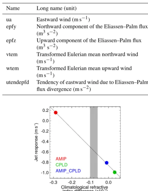
Figure 9.Potential emergent constraint on atmospheric response to Arctic sea ice. Dependence of Atlantic jet response to reduced Arc-tic sea ice on the background climatological refractive index
dif-ference between midlatitudes (25–35◦N) and high latitudes (60–
80◦N) at 200 hPa. Grey shading shows the observed range from the
ERA-Interim and NCEP II reanalyses. The Atlantic jet response is defined as the difference in zonal mean zonal wind at 200 hPa over
the region 50–60◦N, 60–0◦W between model experiments with
reduced and climatological Arctic sea ice. Experiments were per-formed with the same model but with three different configurations: atmosphere only (AMIP); fully coupled (CPLD); and atmosphere only but with SST biases from the coupled model (AMIP_CPLD). An “emergent constraint” is obtained where the observed refractive index difference (grey shading) intersects the simulated response (black line), suggesting a modest weakening of the Atlantic jet in response to reduced Arctic sea ice. Source: Smith et al. (2017).
able information for interpreting the PAMIP experiments. The DECK AMIP experiment forms the basis for PAMIP ex-periment set 5, and the coupled model historical simulation is required to provide starting conditions for experiment sets 2 and 6.
PAMIP will compliment other CMIP6 MIPs, several of which will also provide valuable information on the causes and consequences of polar amplification. In particular, the
magnitudes of polar amplification simulated by different models in response to future and past radiative forcings will be assessed from Scenario MIP (O’Neill et al., 2016) and Paleoclimate MIP (Kageyama et al., 2018). The roles of ex-ternal factors including solar variability, volcanic eruptions, ozone, anthropogenic aerosols and greenhouse gases in driv-ing polar amplification will be studied usdriv-ing experiments proposed in Detection and Attribution MIP (Gillett et al., 2016), Geoengineering MIP (Kravitz et al., 2015), Aerosols and Chemistry MIP (Collins et al., 2017) and Volcanic Forc-ings MIP (Zanchettin et al., 2016); and the roles of AMV and PDV will be studied using experiments proposed by the DCPP (Boer et al., 2016) and Global Monsoons MIP (Zhou et al., 2016).
The impacts of polar amplification on polar ice sheets and carbon uptake will be investigated by the Ice Sheet MIP (Nowicki et al., 2016) and the Coupled Climate–Carbon Cy-cle MIP (Jones et al., 2016a), respectively. Some information on the impacts of reduced sea ice on the atmospheric circu-lation can be obtained from experiments proposed by Cloud Feedback MIP (CFMIP; Webb et al., 2017) in which an at-mosphere model is run twice, forced by the same SSTs but different sea ice concentration fields. However, the CFMIP experiments are not specifically designed to investigate the response to sea ice, and interpreting them is complicated by the fact that the forcing fields will be different for each model.
Improved understanding of the causes and consequences of polar amplification gained through PAMIP and other MIPs will help to interpret decadal predictability diagnosed in DCPP and will reduce the uncertainties in future projections of climate change in polar regions and associated climate impacts, thereby contributing to the Vulnerability, Impacts, Adaptation, and Climate Services (VIACS) Advisory Board (Ruane et al., 2016).
8 Summary
Understanding the causes of polar amplification, and the drivers of recent trends in both the Arctic and Antarctic, rep-resents a key scientific challenge and is important for reduc-ing the uncertainties in projections of future climate change. Several different feedback mechanisms, operating at both high and low latitudes, have been identified but their relative roles are uncertain. Recent trends have also been influenced by external factors other than greenhouse gases, including aerosols, ozone and solar variations, and by changes in at-mosphere and ocean circulations. A key uncertainty is the relative role of local processes that directly affect the surface energy budget and remote processes that affect the poleward atmospheric heat transport. This balance helps to highlight the main feedbacks and processes that drive polar amplifica-tion, and can easily be assessed in numerical model exper-iments by separately imposing changes in sea ice concen-tration and remote SSTs. Such experiments have been per-formed in recent studies (Screen et al., 2012; Perlwitz et al., 2015), but additional models are needed to obtain robust re-sults. PAMIP will therefore provide a robust multi-model as-sessment of the roles of local sea ice and remote SSTs in driv-ing polar amplification. The tier 1 experiments focus on the changes between pre-industrial and present-day conditions, while lower-tier experiments enable recent decades and fu-ture conditions to be investigated.
There is mounting evidence that polar amplification will affect the atmosphere and ocean circulation, with poten-tially important climate impacts in both the midlatitudes and the tropics. In particular, polar amplification will re-duce the Equator-to-pole surface temperature gradient which might be expected to weaken midlatitude westerly winds, promoting cold winters in parts of Europe, North Amer-ica and Asia. Furthermore, enhanced warming of the North-ern Hemisphere relative to the SouthNorth-ern Hemisphere might be expected to shift tropical rainfall northwards and po-tentially influence tropical storm activity. However, despite many studies and intensive scientific debate, there is a lack of consensus on the impacts of reduced sea ice cover in cli-mate model simulations, and the physical mechanisms are not fully understood. There are many potential reasons for disparity across models, including differences in the mag-nitude and pattern of sea ice changes considered, how the changes are imposed, the use of atmosphere-only or cou-pled models, and whether other forcings such as greenhouse gases are included. Hence, coordinated model experiments are needed and will be performed in PAMIP. The tier 1 ex-periments involve atmosphere-only models forced with dif-ferent combinations of sea ice and/or sea surface tempera-tures representing present-day, pre-industrial and future con-ditions. The use of three periods allows the signals of interest to be diagnosed in multiple ways. Lower-tier experiments are proposed to investigate additional aspects and provide further understanding of the physical processes. Specific questions addressed by these are as follows: what role does ocean– atmosphere coupling play in the response to sea ice? How
and why does the atmospheric response to Arctic sea ice de-pend on the pattern of sea ice forcing? How and why does the atmospheric response to Arctic sea ice depend on the model background state? What has been the response to sea ice over the recent period since 1979? How does the response to sea ice evolve on decadal and longer timescales?
A key goal of PAMIP is to determine the real-world situ-ation. Although the experiments proposed here form a coor-dinated set, we anticipate large spread across models. How-ever, this spread will be exploited by seeking “emergent con-straints” in which the real-world situation is inferred from observations of a physical quantity that explains the model differences. For example, if differences in the midlatitude wind response to Arctic sea ice are caused by differences in the refraction of atmospheric waves across models, then ob-servations of the refractive index may provide a constraint on the real-world response. In this way, improved process under-standing gained through analysis of the unprecedented multi-model simulations generated by PAMIP will enable uncer-tainties in projections of future polar climate change and as-sociated impacts to be reduced, and better climate models to be developed.
Appendix A: SIC, SIT and SST forcing data
Forcing fields for the PAMIP experiments are available from the input4MIPs data server (https://esgf-node.llnl.gov/ search/input4mips/, last access: 20 March 2019). Filenames of forcing data for each PAMIP experiment are provided in Table A1. The derivation of forcing data is described here.
Monthly mean fields of SIC, SIT and SST are required for the present-day, pre-industrial and future periods. For SST and SIC, present-day fields are obtained from the observations, using the 1979–2008 climatology from the Hadley Centre Sea Ice and Sea Surface Temperature data set (HadISST; Rayner et al., 2003). For SIT over the Arc-tic, present-day fields are obtained from the Pan-Arctic Ice Ocean Modeling and Assimilation System (PIOMAS; Zhang and Rothrock, 2003). Future and pre-industrial fields are ob-tained from the ensemble of 31 historical and RCP8.5 simu-lations from CMIP5 (see list of models in Table A2). How-ever, models show a large spread in simulations of sea ice, so that a simple ensemble mean would produce an unrealis-tically diffuse ice edge. To obtain a more realistic ice edge, we use present-day observations to constraint the models, as follows:
– We define absolute global mean temperatures represent-ing pre-industrial (13.67◦C), present-day (14.24◦C) and future (2◦warming, 15.67◦C) periods. The present-day global mean temperature corresponds to the 1979– 2008 average from HadCRUT4 observations (Morice et al., 2012). The pre-industrial global mean temperature is obtained by removing from this present-day value an estimate of the global warming index (Haustein et al., 2017) for the period 1979–2008 (0.57◦C). The future global mean temperature is defined as+2◦C from the pre-industrial period, i.e. 15.67◦C.
– For each model, find the periods when the 30-year mean global temperature equals the above values and compute the 30-year averaged fields.
– At each grid point, use the observed present-day value to constrain the model simulations of future and pre-industrial conditions. This is achieved by computing a linear regression across the models between future (or pre-industrial) and present-day values simulated by the model ensemble, and taking the required future (or pindustrial) estimate as the point where this regression re-lationship intersects the observed present-day value. We use quantile regression rather than least squares regres-sion to reduce the impact of outliers and hence provide a sharper ice edge. This procedure is used to create past and future SIC/SST/SIT fields, with the quantile of the regression being chosen to increase the signal. For the future, the lower (upper) quartile regression is used for SIC/SIT (SST), in order to give more weight to models with less sea ice and warmer SST. Conversely, for the
pre-industrial period, the upper (lower) quartile is used for SIC/SIT (SST), giving more weight to models with larger sea ice and cooler SST.
Some experiments, such as 1.6, require SSTs to be speci-fied in regions where the sea ice has been removed. We fol-low the methodology of Screen et al. (2013); i.e. we impose pre-industrial/future SST (derived from the quantile regres-sion) in grid points where pre-industrial/future SIC deviates by more than 10 % of its present-day value. Example SIC and SST fields are shown in Figs. 5–8.
In experiment 3, future sea ice changes are only imposed in the Barents/Kara seas and Sea of Okhotsk. Future SIC fields for these experiments were created by replacing present-day values with future values but only in the required regions, defined as 65–85◦N, 10–110◦E for the Barents/Kara seas and 40–63◦N, 135–165◦E for the Sea of Okhotsk.
For experiment 5, monthly mean SST and SIC climatolo-gies were created from the CMIP6 AMIP data. For 5.1, SST is set to the transient values where sea ice substantially de-viates (by more than 10 %) from climatology. For 5.2, SST is set to the transient values where sea ice is absent in the climatology but present in the transient fields, and−1.8◦C where sea ice is present in the climatology but absent in the transient fields.
For experiments 1.9 and 1.10, SIT in the Arctic is derived from PIOMAS. Since no SIT observations are available in the Antarctic, we use the median of present-day values sim-ulated by the model ensemble. The same present-day SIT values are used in the Antarctic in the SIT forcing field of experiments 6.1 and 6.2. For experiment 6.3 (future Antarc-tic SIC/SIT), we use the lower quartile of future values sim-ulated by the model ensemble. Where SIC is greater than 15 %, but SIT equals 0, SIT is set to 15 cm.
Appendix B: Experiment details AMIP II
Before use, the forcing data (SST, SIC and SIT) should be processed following the standard AMIP II protocol (Taylor et al., 2000). This is to ensure that monthly means computed from the model (after interpolating to the required model time steps) agree with the monthly means in the forcing files. Radiative forcing
Table A1.Names of forcing files for each experiment. Files are available from the input4MIPs data server (https://esgf-node.llnl.gov/search/ input4mips/last access: 20 March 2019). Comments in square brackets are optional guidance for groups that are able to constrain sea ice thickness (sithick).
No. Experiment name Names of forcing files
1.1 pdSST-pdSIC tos_input4MIPs_SSTsAndSeaIce_PAMIP_UCI-present-1-0_gn_197901-200812-clim.nc
siconc_input4MIPs_SSTsAndSeaIce_PAMIP_UCI-present-1-0_gn_197901-200812-clim.nc
1.2 piSST-piSIC tos_input4MIPs_SSTsAndSeaIce_PAMIP_UCI-preindustrial-1-0_gn_187001-188012-clim.nc
siconc_input4MIPs_SSTsAndSeaIce_PAMIP_UCI-preindustrial-1-0_gn_187001-188012-clim.nc
1.3 piSST-pdSIC tos_input4MIPs_SSTsAndSeaIce_PAMIP_UCI-pi-prArctic-prAntarctic-1-0_gn_187001-188012-clim.nc
siconc_input4MIPs_SSTsAndSeaIce_PAMIP_UCI-present-1-0_gn_197901-200812-clim.nc
1.4 futSST-pdSIC tos_input4MIPs_SSTsAndSeaIce_PAMIP_UCI-fu-prArctic-prAntarctic-1-0_gn_clim.nc
siconc_input4MIPs_SSTsAndSeaIce_PAMIP_UCI-present-1-0_gn_197901-200812-clim.nc
1.5 pdSST-piArcSIC tos_input4MIPs_SSTsAndSeaIce_PAMIP_UCI-piArctic-1-0_gn_187001-188012-clim.nc
siconc_input4MIPs_SSTsAndSeaIce_PAMIP_UCI-piArctic-1-0_gn_187001-188012-clim.nc
1.6 pdSST-futArcSIC tos_input4MIPs_SSTsAndSeaIce_PAMIP_UCI-fut2CArctic-1-0_gn_clim.nc
siconc_input4MIPs_SSTsAndSeaIce_PAMIP_UCI-fut2CArctic-1-0_gn_clim.nc
1.7 pdSST-piAntSIC tos_input4MIPs_SSTsAndSeaIce_PAMIP_UCI-piAntarctic-1-0_gn_187001-188012-clim.nc
siconc_input4MIPs_SSTsAndSeaIce_PAMIP_UCI-piAntarctic-1-0_gn_187001-188012-clim.nc
1.8 pdSST-futAntSIC tos_input4MIPs_SSTsAndSeaIce_PAMIP_UCI-fut2CAntarctic-1-0_gn_clim.nc
siconc_input4MIPs_SSTsAndSeaIce_PAMIP_UCI-fut2CAntarctic-1-0_gn_clim.nc
1.9 pdSST-pdSICSIT tos_input4MIPs_SSTsAndSeaIce_PAMIP_UCI-present-1-0_gn_197901-200812-clim.nc
siconc_input4MIPs_SSTsAndSeaIce_PAMIP_UCI-present-1-0_gn_197901-200812-clim.nc
sithick_input4MIPs_SSTsAndSeaIce_PAMIP_UCI-present-2mAntarctic-1-0_gn_197901-200812-clim.nc
1.10
pdSST-futArcSICSIT
tos_input4MIPs_SSTsAndSeaIce_PAMIP_UCI-fut2CArctic-1-0_gn_clim.nc siconc_input4MIPs_SSTsAndSeaIce_PAMIP_UCI-fut2CArctic-1-0_gn_clim.nc
sithick_input4MIPs_SSTsAndSeaIce_PAMIP_UCI-fut2CArctic-2mAntarctic-1-0_gn_clim.nc
2.1 pa-pdSIC siconc_input4MIPs_SSTsAndSeaIce_PAMIP_UCI-present-1-0_gn_197901-200812-clim.nc
(sithick as used in experiment 1.1)
2.2 pa-piArcSIC siconc_input4MIPs_SSTsAndSeaIce_PAMIP_UCI-piArctic-1-0_gn_187001-188012-clim.nc
(sithick as used in experiment 1.5)
2.3 pa-futArcSIC siconc_input4MIPs_SSTsAndSeaIce_PAMIP_UCI-fut2CArctic-1-0_gn_clim.nc (sithick as used in
experi-ment 1.6)
2.4 pa-piAntSIC siconc_input4MIPs_SSTsAndSeaIce_PAMIP_UCI-piAntarctic-1-0_gn_187001-188012-clim.nc
(sithick as used in experiment 1.7)
2.5 pa-futAntSIC siconc_input4MIPs_SSTsAndSeaIce_PAMIP_UCI-fut2CAntarctic-1-0_gn_clim.nc
(sithick as used in experiment 1.8)
3.1
pdSST-futOkhotskSIC
tos_input4MIPs_SSTsAndSeaIce_PAMIP_UCI-fut2COkhotsk-1-0_gn_clim.nc siconc_input4MIPs_SSTsAndSeaIce_PAMIP_UCI-fut2COkhotsk-1-0_gn_clim.nc
3.2
pdSST-futBKSeasSIC
tos_input4MIPs_SSTsAndSeaIce_PAMIP_UCI-fut2CBKSeas-1-0_gn_clim.nc siconc_input4MIPs_SSTsAndSeaIce_PAMIP_UCI-fut2CBKSeas-1-0_gn_clim.nc
4.1 modelSST-pdSIC tos to be created from experiment 2.1 as described in Appendix B
siconc_input4MIPs_SSTsAndSeaIce_PAMIP_UCI-present-1-0_gn_197901-200812-clim.nc
4.2
modelSST-futArcSIC
tos to be created from experiment 2.1 as described in Appendix B
Table A1.Continued.
No. Experiment name Names of forcing files
5.1 amip-climSST
tos_input4MIPs_SSTsAndSeaIce_PAMIP_UCI-present-197901-201412-Arctic-Antarctic-1-0_gn_197901-201412-clim.nc
siconc_input4MIPs_SSTsAndSeaIce_PAMIP_UCI-present-1-0_gn_197901-201412.nc
5.2 amip-climSIC
tos_input4MIPs_SSTsAndSeaIce_PAMIP_UCI-present-197901-201412-clim-Arctic-Antarctic-1-0_gn_197901-201412.nc
siconc_input4MIPs_SSTsAndSeaIce_PAMIP_UCI-present-1-0_gn_197901-201412-clim.nc
6.1 pa-pdSIC-ext siconc_input4MIPs_SSTsAndSeaIce_PAMIP_UCI-present-1-0_gn_197901-200812-clim.nc
(sithick_input4MIPs_SSTsAndSeaIce_PAMIP_UCI-present-1-0_gn_197901-201412-clim.nc)
6.2 pa-futArcSIC-ext siconc_input4MIPs_SSTsAndSeaIce_PAMIP_UCI-fut2CArctic-1-0_gn_clim.nc
(sithick_input4MIPs_SSTsAndSeaIce_PAMIP_UCI-fut2CArctic-1-0_gn_clim.nc)
6.3 pa-futAntSIC-ext siconc_input4MIPs_SSTsAndSeaIce_PAMIP_UCI-fut2CAntarctic-1-0_gn_clim.nc
(sithick_input4MIPs_SSTsAndSeaIce_PAMIP_UCI-fut2CAntarctic-1-0_gn_clim.nc)
Start date and length of simulations
Experiments 1 to 4 should start on 1 April 2000 and run for 14 months, with the first 2 months ignored to allow for an ini-tial model spin-up. Experiment 6 starts at the same time but extends to 100 years. Experiment 5 starts on 1 January 1979 and ends on 31 December 2014 in accordance with the AMIP protocol (Eyring et al., 2016).
Initial conditions and ensemble generation
Initial conditions for atmosphere-only experiments (1, 3 and 4) should be based on the AMIP simulation for 1 April 2000 if possible, though any suitable start dump may be used, noting that the first 2 months of the simulations will be ig-nored. Initial conditions for the coupled experiments (2 and 6) should be based on 1 April 2000 from the CMIP6 histor-ical simulation (Eyring et al., 2016). Ideally, different ocean states will be sampled by using different ensemble members of the historical simulation if these are available. Large en-sembles (∼100 members) are requested in order to obtain statistically robust results, since models typically simulate a small atmospheric response to sea ice relative to internal variability (Screen et al., 2014; Mori et al., 2014). We note that this may not be the case in reality, since models under-estimate the signal-to-noise ratio in seasonal and interannual forecasts of the NAO (Scaife et al., 2014; Eade et al., 2014; Dunstone et al., 2016). The results are not expected to be par-ticularly sensitive to the way in which ensemble members are generated, and any suitable method may be used but should be documented.
Frequency of boundary conditions
SST and sea ice boundary conditions are specified as monthly means and should be interpolated to the required model time step (as is standard practice). Daily boundary
conditions might strengthen some of the signals, but the addi-tional complexity was considered unnecessary for assessing the physical processes and signals of interest here.
Constraining sea ice in coupled models
Table A2.List of models used to construct the forcing fields.
Acronym Research centre ACCESS1-0
Commonwealth Scientific and Industrial Research Organisation, and Bureau of Meteorology, Australia ACCESS1-3
bcc-csm1-1
Beijing Climate Center, China bcc-csm1-1-m
CanESM2 Canadian Centre for Climate Modelling and Analysis, Canada CCSM4
National Center for Atmospheric Research, USA CESM1-BGC
CESM1-CAM5 CMCC-CM
Centro Euro-Mediterraneo per I Cambiamenti Climatici, Italy CMCC-CMS
CNRM-CM5 Centre National de Recherches Météorologiques/Centre Européen de Recherche et Formation Avancées en Calcul Scientifique, France CSIRO-Mk3-6-0 Commonwealth Scientific and Industrial Research Organisation, in collaboration with the Queensland Climate Change Centre of
Excel-lence, Australia EC-EARTH EC-Earth
FIO-ESM The First Institute of Oceanography, China GFDL-CM3
GFDL-ESM2G US Department of Commerce/National Oceanic and Atmospheric Administration/Geophysical Fluid Dynamics Laboratory, USA GFDL-ESM2M
GISS-E2-H
National Aeronautics and Space Administration/Goddard Institute for Space Studies, USA GISS-E2-R
HadGEM2-CC
Met Office Hadley Centre, UK HadGEM2-ES
inmcm4 Institute for Numerical Mathematics, Russia IPSL-CM5A-LR
Institut Pierre Simon Laplace, France IPSL-CM5A-MR
IPSL-CM5B-LR
MIROC5 Center for Climate System Research (University of Tokyo), National Institute for Environmental Studies, and Frontier Research Center for Global Change, Japan
MPI-ESM-LR
Max Planck Institute for Meteorology, Germany MPI-ESM-MR
MRI-CGCM3 Meteorological Research Institute, Japan NorESM1-M
Sea ice thickness
Some participating groups may not able to specify sea ice thickness. Hence, in the atmosphere-only experiments (ex-cept 1.9 and 1.10), sea ice thickness should be treated in the same way as in the AMIP DECK simulation. We note that there is not a common protocol, but in practice the sea ice thickness will be at least 2 m so that differences in sur-face fluxes between models will be small. Experiments 1.9 and 1.10 are designed to investigate the impacts of future sea ice thickness changes, and sea ice thickness should be con-strained with a relaxation timescale (or equivalent flux) of 5 days. Groups that are able to specify sea ice thickness are requested to do so for the coupled model experiments, using values from the equivalent atmosphere-only simulations for experiment 2, and the fields provided by PAMIP for experi-ment 6. If sea ice thickness cannot be specified, then it should be left free to evolve in the coupled model experiments. SST forcing fields for experiment set 4
Author contributions. All authors contributed to the design of the experimental protocol. DMS led the writing with comments from all authors. YP created the forcing data in collaboration with DMS, JAS and TJ.
Competing interests. The authors declare that they have no conflict of interest.
Acknowledgements. The author give thanks to the US CLIVAR
Working Group on Arctic Change and the Aspen Global Change In-stitute (AGCI) for hosting workshops which contributed to PAMIP planning, with funding from NASA, NSF, NOAA and DOE. Doug M. Smith was supported by the joint DECC/Defra Met Office Hadley Centre Climate Programme (GA01101) and the EU H2020 APPLICATE project (GA727862). James A. Screen was supported by NERC grant NE/R005125/1. NCAR is sponsored by the Na-tional Science Foundation. Javier García-Serrano was supported by the EU H2020 PRIMAVERA (GA641727). Jin-Ho Yoon was sup-ported by the funding from the Korean Polar Research Institute through grant PE16100. Daniela Matei was supported by the EU H2020 Blue-Action (GA 727852) and BMBF project CLIMPRE InterDec (FKZ:01LP1609A). Jinro Ukita was supported by ArCS and InderDec. The authors thank Yannick Peings for creating the forcing fields.
Review statement. This paper was edited by Julia Hargreaves and Lauren Gregoire and reviewed by two anonymous referees.
References
Acosta Navarro, J. C., Varma, V., Riipinen, I., Seland, Ø., Kirkevåg, A., Struthers, H., Iversen, T., Hansson H.-C., and Ekman, A. M. L.: Amplification of Arctic warming by past air pollution reductions in Europe, Nat. Geosci., 9, 277–281, https://doi.org/10.1038/ngeo2673, 2016.
Alexander, M. A., Bhatt, U. S., Walsh, J. E., Timlin, M. S., Miller, J. S., and Scott, J. D.: The atmospheric response to realistic Arctic sea ice anomalies in an AGCM during winter, J. Clim., 17, 890– 905, 2004.
Armour, K. C., Marshall, J., Scott, J., Donohoe A., and Newsom, E. R.: Southern Ocean warming delayed by circumpolar up-welling and equatorward transport, Nat. Geosci., 9, 549–554, https://doi.org/10.1038/ngeo2731, 2016.
Bader, J., Flügge, M., Kvamstø, N. G., Mesquita M. D. S., and Voigt, A.: Atmospheric winter response to a projected future Antarctic sea-ice reduction: a dynamical analysis, Clim. Dynam., 40, 2707–2718, 2013.
Balmaseda, M. A., Ferranti, L., Molteni F., and Palmer, T. N.: Im-pact of 2007 and 2008 Arctic ice anomalies on the atmospheric circulation: Implciations for long-range predictions, Q. J. Roy. Meteor. Soc., 136, 1655–1664, 2010.
Barnes, E. A. and Screen, J. A.: The impact of Arctic warming on the midlatitude jet-stream: Can it? Has it? Will it?, Clim. Change, 6, 277–286, https://doi.org/10.1002/wcc.337, 2015.
Bindoff, N. L., Stott, P. A., Achuta Rao, K. M., Allen, M. R., Gillett, N., Gutzler, D., Hansingo, K., Hegerl, G., Hu, Y., Jain, S., Mokhov, I. I., Overland, J., Perlwitz, J., Sebbari R., and Zhang, X.: Detection and Attribution of Climate Change: from Global to Regional, in: Climate Change 2013: The Physical Science Basis, Contribution of Working Group I to the Fifth Assessment Report of the Intergovernmental Panel on Climate Change, edited by: Stocker, T. F., Qin, D., Plattner, G.-K., Tignor, M., Allen, S. K., Boschung, J., Nauels, A., Xia, Y., Bex, V., and Midgley, P. M., Cambridge University Press, Cambridge, UK, New York, NY, USA, 2013.
Bintanja, R., van Oldenborgh, G. J., Drijfhout, S. S., Wouters, B., and Katsman, C. A.: Important role for ocean warming and increased ice-shelf melt in Antarctic sea-ice expansion, Nat. Geosci., 6, 376–379, 2013.
Blackport, R. and Kushner, P.: The transient and equilibrium cli-mate response to rapid summertime sea ice loss in CCSM4, J. Clim., 29, 401–417, https://doi.org/10.1175/JCLI-D-15-0284.1, 2016.
Blackport, R. and P. J. Kushner: Isolating the atmospheric circula-tion response to Arctic sea ice loss in the coupled climate sys-tem, J. Clim., 30, 2163–2185, https://doi.org/10.1175/JCLI-D-16-0257.1, 2017.
Boer, G. J., Smith, D. M., Cassou, C., Doblas-Reyes, F., Danaba-soglu, G., Kirtman, B., Kushnir, Y., Kimoto, M., Meehl, G. A., Msadek, R., Mueller, W. A., Taylor, K. E., Zwiers, F., Rixen, M., Ruprich-Robert, Y., and Eade, R.: The Decadal Climate Predic-tion Project (DCPP) contribuPredic-tion to CMIP6, Geosci. Model Dev., 9, 3751–3777, https://doi.org/10.5194/gmd-9-3751-2016, 2016. Bracegirdle, T. J. and Stephenson, D. B.: On the robustness of
emer-gent constraints used in multimodel climate change projections of Arctic warming, J. Clim. 26, 669–678, 2013.
Cassano, E. N., Cassano, J. J., Higgins, M. E., and Serreze, M. C.: Atmospheric impacts of an Arctic sea ice minimum as seen in the Community Atmosphere Model, Int. J. Climatol., 34, 766–779, https://doi.org/10.1002/joc.3723, 2014.
Chen, H. W., Zhang, F., and Alley, R. B.: The robustness of mid-latitude weather pattern changes due to Arctic sea ice loss, J. Climate, 29, 7831–7849, https://doi.org/10.1175/JCLI-D-16-0167.1, 2016.
Chiang, J. C. H. and Bitz, C. M.: Influence of high latitude ice on the marine intertropical convergence zone, Clim. Dynam., 25, 477– 496, https://doi.org/10.1007/s00382-005-0040-5, 2005. Chylek, P., Folland, C. K., Lesins, G., Dubey, M. K., and Wang,
M.: Arctic air temperature change amplification and the At-lantic Multidecadal Oscillation, Geophys. Res. Lett., 36, L14801, https://doi.org/10.1029/2009GL038777, 2009.
Cohen, J. and Entekhabi, D.: Eurasian snow cover variability and Northern Hemisphere climate predictability, Geophys. Res. Lett., 26, 345–348, https://doi.org/10.1029/1998GL900321, 1999. Cohen, J., Jones, J., Furtado, J. C., and Tziperman, E.: Warm Arctic,
cold continents: A common pattern related to Arctic sea ice melt, snow advance, and extreme winter weather, Oceanography, 26, 150–160, https://doi.org/10.5670/oceanog.2013.70, 2013. Cohen, J., Screen, J. A., Furtado, J. C., Barlow, M.,