https://doi.org/10.5194/gmd-12-3241-2019 © Author(s) 2019. This work is distributed under the Creative Commons Attribution 4.0 License.
Max Planck Institute Earth System Model (MPI-ESM1.2) for the
High-Resolution Model Intercomparison Project (HighResMIP)
Oliver Gutjahr1, Dian Putrasahan1, Katja Lohmann1, Johann H. Jungclaus1, Jin-Song von Storch1, Nils Brüggemann1,2, Helmuth Haak1, and Achim Stössel3
1The Ocean in the Earth System, Max Planck Institute for Meteorology, Hamburg, Germany 2Institut für Meereskunde, Universität Hamburg, Hamburg, Germany
3Department of Oceanography, Texas A&M University, College Station, TX, USA
Correspondence:Oliver Gutjahr ([email protected]) Received: 14 November 2018 – Discussion started: 17 December 2018 Revised: 4 July 2019 – Accepted: 4 July 2019 – Published: 25 July 2019
Abstract. As a contribution towards improving the climate mean state of the atmosphere and the ocean in Earth sys-tem models (ESMs), we compare several coupled simula-tions conducted with the Max Planck Institute for Meteorol-ogy Earth System Model (MPI-ESM1.2) following the High-ResMIP protocol. Our simulations allow to analyse the sep-arate effects of increasing the horizontal resolution of the ocean (0.4 to 0.1◦) and atmosphere (T127 to T255) submod-els, and the effects of substituting the Pacanowski and Phi-lander (PP) vertical ocean mixing scheme with the K-profile parameterization (KPP).
The results show clearly distinguishable effects from all three factors. The high resolution in the ocean removes bi-ases in the ocean interior and in the atmosphere. This leads to the important conclusion that a high-resolution ocean has a major impact on the mean state of the ocean and the atmo-sphere. The T255 atmosphere reduces the surface wind stress and improves ocean mixed layer depths in both hemispheres. The reduced wind forcing, in turn, slows the Antarctic Cir-cumpolar Current (ACC), reducing it to observed values. In the North Atlantic, however, the reduced surface wind causes a weakening of the subpolar gyre and thus a slowing down of the Atlantic meridional overturning circulation (AMOC), when the PP scheme is used. The KPP scheme, on the other hand, causes stronger open-ocean convection which spins up the subpolar gyres, ultimately leading to a stronger and sta-ble AMOC, even when coupled to the T255 atmosphere, thus retaining all the positive effects of a higher-resolved atmo-sphere.
1 Introduction
The evolving computational power allows for ever-higher resolutions of Earth system models (ESMs). High-resolution ESMs are able to explicitly resolve processes that are at sub-grid scale and parameterized in low-resolution models. Opti-mally, better resolved processes would improve atmosphere and ocean dynamics and thus reduce biases in the mean state and in the variability of key quantities. In this paper, we separately increase the horizontal resolution of the atmo-sphere and ocean submodels and analyse the effects on the mean states. Besides increasing the resolution of the major model subcomponents, new strategies and model develop-ments, such as improved physics, are required for improv-ing ESMs. Therefore, we also analyse the effects of a more sophisticated vertical mixing parameterization in the ocean submodel.
Table 1.Overview of MPI-ESM1.2 control simulations used within this study and their horizontal resolutions. The number of vertical levels is 95 in the atmosphere and 40 in the ocean, respectively. In brackets, the nominal horizontal resolution in a Gaussian grid (approximated at the Equator) is given. All models use 30 years of spin-up and are analysed for the subsequent 50 years.
Name Atmosphere resolution Ocean resolution Ocean mixing Description scheme
HR T127 (0.93◦or∼103 km) TP04 (0.4◦or∼44 km) PP, KPP Reference, ocean mixing sensitivity XR T255 (0.46◦or∼51 km) TP04 (0.4◦or∼44 km) PP, KPP Increased atmospheric resolution,
ocean mixing sensitivity ER T127 (0.93◦or∼103 km) TP6M (0.1◦or∼11 km) PP Increased ocean resolution
All our simulations follow the High Resolution Model Intercomparison Project (HighResMIP) protocol (Haarsma et al., 2016) and provide climate simulations with varying horizontal resolutions that are higher than the standard resolution of the Coupled Model Intercomparison Project – phase 6 (CMIP6; Eyring et al., 2016). An overview of all performed simulations for this study is shown in Table 1.
Our reference model is the MPI-ESM1.2-HR (or HR in the remainder of the paper), which was recently described by Müller et al. (2018) and contributes to CMIP6. HR is the higher-resolution version of the former MPI-ESM1.2-LR (or LR), with 1.5 times as high (T127,∼100 km) horizontal res-olution for the atmospheric submodel ECHAM6.3 (Hertwig et al., 2015; Mauritsen et al., 2018) and a 0.4◦ (∼40 km) ocean on an eddy-permitting tripolar grid (TP04) (Jungclaus et al., 2013) compared to the LR version (T63,∼200 km at-mosphere and 1.5◦ ocean grid). How the ocean and atmo-sphere mean states improve in HR compared to LR was de-scribed by Müller et al. (2018).
Further reductions of atmospheric biases were shown by Hertwig et al. (2015), who used ECHAM6.3 with a T255 (∼
50 km) resolution in the Atmospheric Model Intercompari-son Project (AMIP)-type experiments. Building on these im-provements, we further use a coupled MPI-ESM1.2 version with the T255 atmosphere and the TP04 ocean grid (MPI-ESM1.2-XR or simply XR) to investigate the effect of an increased atmospheric resolution on the mean state. This XR version was already used by Putrasahan et al. (2019) and (al-though under a different acronym) by Milinski et al. (2016). Milinski et al. (2016) demonstrated that the sea surface tem-perature bias in the upwelling regions along the coast of Africa diminished because of a more detailed representation of the coastal winds with the T255 atmosphere. Although bi-ases were reduced with a T255 version of ECHAM6.3, our XR simulation generally produces too-weak surface wind speeds, in particular over the North Atlantic and the subpolar gyre (Putrasahan et al., 2019).
These weaker near-surface winds caused a slowdown of the AMOC to about 9 Sv (Sv:=106m3s−1), as documented by Putrasahan et al. (2019). This issue was not only affecting the MPI-ESM1.2 but was also reported by other modelling
centres using ECHAM6, although going from T63 to T127 (Sein et al., 2018). Sein et al. (2018) gave a possible expla-nation for the reduction of mean wind speeds, which they at-tribute to a higher cyclone activity with the T127 resolution, in particular over the North Atlantic.
The AMOC strength and its stability depend to a large ex-tent on the vertical mixing parameterization (Gent, 2018). To investigate the sensitivity of the AMOC and the mean states, we conducted parallel experiments with HR and XR in which the modified parameterization of Pacanowski and Phi-lander (1981) (PP), which is default in MPI-ESM1.2 (Mars-land et al., 2003), was replaced by the more sophisticated K-profile parameterization (KPP) scheme of Large et al. (1994). It turned out that the KPP scheme compensates for the under-estimated mean winds in the high latitudes and in the tropics in the XR simulation, sustaining a stable AMOC. The rea-sons for this will be elaborated upon.
Finally, we adopt the 0.1◦(∼10 km) tripolar grid (TP6M) of MPIOM, which was already used in an ocean-only sim-ulation forced by NCEP, and in a coupled run with T63 and T255 versions of ECHAM6 – the so-called STORM simulations (von Storch et al., 2012; Stössel et al., 2015, 2018). With this high-resolution, mostly eddy-resolving cou-pled version (MPI-ESM1.2-ER or ER), we detect noticeable reductions of biases not only in the ocean and near-surface atmosphere but also in the higher atmosphere. This leads to the important conclusion that high resolution in the ocean has a major impact on the large-scale temperature distribution in the atmosphere, consistent with recent findings (Frenger et al., 2013; Ma et al., 2016; Liu et al., 2018). The parallel simulations allow to separately analyse (1) the effects of in-creased atmospheric resolution (HR vs. XR), (2) the effects of increased ocean model resolution (HR vs. ER), and (3) the effect of an alternative vertical ocean mixing parameteriza-tions (PP vs. KPP) on the mean climate.
effects from increased resolution with improved ocean mix-ing.
2 Model, spin-up, and experiments 2.1 Model description
The atmospheric submodel of MPI-ESM1.2 is ECHAM6.3 (Mauritsen et al., 2018), which includes the land-surface scheme JSBACH (Stevens et al., 2013; Reick et al., 2013). The ocean and sea ice submodels are combined in MPIOM (Jungclaus et al., 2013; Notz et al., 2013). ECHAM6.3 and MPIOM are coupled via the Ocean-Atmosphere-Sea-Ice coupler version 3 (OASIS3-mct; Valcke, 2013) with a cou-pling frequency of 1 h. ECHAM6.3 was used with 95 verti-cal levels at two different spectral resolutions, truncated at T127 (∼103 km) in HR and ER and T255 (∼51 km) in XR. We did not change any parameter going from HR to XR, except for a reduction of the time step from 200 s (HR) to 90 s (XR) and the horizontal diffusion damping term. Both use the same eddy-permitting ocean with a resolution of 0.4◦ (∼44 km) on a tripolar grid (TP04; Jungclaus et al., 2013) with 40 unevenly spaced vertical levels. The first 20 levels are distributed in the top 750 m. A partial grid cell formulation (Adcroft et al., 1997; Wolff et al., 1997) is used for a more ac-curate representation of the bottom topography. River runoff is calculated by a horizontal discharge model (Hagemann and Gates, 2003).
In the ER configuration, the ocean component has a nom-inal resolution of 0.1◦(∼10 km) on a tripolar grid (TP6M) (e.g. von Storch et al., 2012, 2016). The TP6M grid is quasi-uniform in the Northern Hemisphere and scales with latitude (0.1◦cos(φ)) in the Southern Hemisphere (von Storch et al.,
2016). The grid size is thus smaller than the nominal res-olution in the Southern Ocean (5 to 6 km near 60◦S) and about 2 to 3 km in the Weddell and Ross seas. The TP6M grid resolves the major bulk of mesoscale eddies but not in the Arctic Ocean and the Nordic Seas, the marginal seas of the subpolar North Atlantic, and on continental shelves.
We did not change any parameters compared to the TP04 grid as prescribed by the HighResMIP protocol (Haarsma et al., 2016), except that we reduced the time step from 3600 s (TP04) to 240 s (TP6M). Table 1 provides an overview of the simulations that we compared in this study. The HR config-uration of our reference simulation is exactly the same as in Müller et al. (2018). The XR configuration was used by Her-twig et al. (2015) (denoted as VHR in their study) for AMIP simulations with ECHAM6 and in Milinski et al. (2016) (denoted as HRatm in their study) for MPI-ESM runs. The TP6M configuration was already used in stand-alone ocean simulations with 80 vertical levels (von Storch et al., 2012; Stössel et al., 2018) and in fully coupled simulations (e.g. Stössel et al., 2015).
All simulations (except ER) use the thickness diffusivity κGM of the Gent et al. (1995) (GM) parameterization to ac-count for the diffusion and tracer advection induced by un-resolved mesoscale eddies in the ocean. For the TP04 grid, κGM is constant and chosen to be proportional to the grid spacing. A value ofκGM=250 m2s−1is chosen for a 400 km wide grid cell and it reduces linearly with increasing resolu-tion. That is, for the eddy-permitting TP04 grid,κGMis only about 10 % of this value. We had two reasons for keeping this rather low GM coefficient compared to what is used by, e.g. Marshall et al. (2017). First, we want to be consistent with previous MPI-ESM simulations, and second, the GM coeffi-cient was used to tune the AMOC, which became too weak in the TP04 configuration with higher values (von Storch et al., 2016). We note that finding an optimal configuration is chal-lenging and still an open issue, in particular for grids that are a mixture of non-resolving, permitting and eddy-resolving parameterizations as our tripolar grids. The TP04 grid is eddy-permitting, so eddies are partly resolved and partly parameterized. Strictly, the same applies to the TP6M grid, which does not resolve eddies in all parts of the ocean, but we decided to switch off GM in this configuration. There are also strategies to completely switch off GM already for eddy-permitting grids (Delworth et al., 2012).
The lateral eddy diffusivity is parameterized by an isopycnal formulation (Redi, 1982) and is set to κRedi= 1000 m2s−1for a 400 km wide grid cell, again reducing lin-early with increasing resolution. In ER,κGM is set to zero, butκRediis unchanged (von Storch et al., 2016).
An innovation over previous versions of HR and XR is that we used two different diapycnal mixing schemes (see Sect. 2.2): the PP scheme as default and the KPP scheme. The diapycnal mixing scheme used in a simulation is indicated by subscripts: HRpp, HRkpp, XRpp, XRkpp, and ERpp. Note that the model was not retuned when the KPP scheme was used, to account for the pure effect of a changed ocean mixed layer scheme. For all our comparisons, HRppis our reference simulation.
2.2 Diapycnal mixing
Previous MPI-ESM versions used a modified version of the Richardson-number-dependent formulation of Pacanowski and Philander (1981) (PP scheme). The modification of the original PP formulation consists of a parameterization for wind-induced mixing that decays exponentially with depth (Marsland et al., 2003). Convection is parameterized by en-hanced eddy diffusivity (kv=0.1 m2s−1). For our simula-tions, we corrected a bug associated with the vertical viscosi-ties, which were only about 50 % of the correct solution from the PP scheme. This error was then also corrected in the HR version described by Müller et al. (2018). The background value for the vertical diffusivity is constant and was set to 1.05×10⁻⁵ and to 5×10⁻⁵m2s−1 for the viscosity. The background values represent the breaking of internal waves, which provide the mechanical energy for diapycnal mixing in the interior of the ocean. The PP scheme is the default option in MPI-ESM1.2 and is thus used in our reference simulation (HRpp).
To improve the diapycnal mixing in MPIOM, we imple-mented the non-local KPP (Large et al., 1994). The KPP scheme was implemented by adding the Community Verti-cal Mixing (CVMix) project library (Griffies et al., 2013) to MPIOM. In the KPP scheme, turbulent transport does not only depend on local gradients of the properties but also on the overall state of the boundary layer, that is the surface fluxes and the boundary layer depth (Large et al., 1994). The non-local turbulent transport represents how surface proper-ties are redistributed from the surface layer into the bound-ary layer, for example, by buoyant plumes, Langmuir cells, or mesoscale cellular convective elements.
The non-local fluxes are non-zero only for tracers in un-stable forcing conditions, i.e. for negative surface buoyancy fluxes. They then directly depend on the net heat and fresh-water fluxes crossing the ocean surface multiplied by the lo-cal vertilo-cal diffusivities, a vertilo-cal shape function, and some constants (Griffies et al., 2013). For these non-local fluxes, the same vertical diffusivities are assumed as for the local tracer diffusion. In contrast to the PP scheme, these diffusiv-ities are not limited to a user-specified value but depend on a depth-dependent turbulent vertical velocity scale, on a ver-tical shape function, and on the mixed layer depth (Griffies et al., 2013).
Below the mixed layer, we use the PP scheme with the same constant background diffusivity and viscosity. The dif-fusivities are not matched at the base of the mixed layer to avoid potential overshooting of the non-local transport terms, which might produce extrema in the tracer field (Griffies et al., 2013). Under sea ice, we reduce the wind-induced mix-ing in the PP and in the KPP scheme, so that the surface fric-tion velocityu∗ decreases quadratically with increasing sea
ice concentration. For simplicity, we neglect that the momen-tum flux from the atmosphere into the ocean could be even stronger when sea ice is present, because of additional
mo-mentum flux at the interface of sea ice and the underlying seawater.
3 Evaluation of the atmospheric mean state
For the evaluation, the MPI-ESM1.2 simulations were aver-aged over the first 50 model years after the spin-up. We used the ERA-Interim reanalysis data (Dee et al., 2011) averaged from 1979 to 2005 as the reference for the atmospheric mean state, as HR was tuned to this period (Mauritsen et al., 2012). 3.1 Surface quantities
3.1.1 10 m wind speed
The time mean of the simulated 10 m scalar wind speed agrees well with ERA-Interim for large parts of the world’s oceans and over the continents (Fig. 1). Consistently too-low wind speeds, however, evolve over the northern parts of America and Europe, over South America, and over Green-land and Antarctica. Too-strong winds are simulated by all model configurations over the subtropical oceans north and south of the Equator. Models with the T127 atmosphere fur-ther simulate too-strong winds speeds over the Weddell Sea (Fig. 1b, c, f).
Overall, the KPP scheme has only a minor effect on the 10 m wind speed. In the equatorial Pacific, KPP reverses the negative bias to a positive wind speed bias. Further, the nega-tive bias in the Denmark and Fram straits is reduced because of lower sea ice concentration in this area (see Sect. 4.4).
Increasing the horizontal resolution from T127 to T255 in XRpp(Fig. 1d) introduces a negative wind speed bias over the Antarctic Circumpolar Current (ACC) because of a reduced meridional pressure gradient. The near-surface wind speeds are further too low over the subpolar gyre in the North At-lantic and over the Nordic Seas. This reduced wind stress over the subpolar gyre causes a slowdown of the AMOC in XRpp, as described in detail by Putrasahan et al. (2019).
By using the KPP scheme in the XR model (XRkpp; Fig. 1e), the wind speed is too weak but not as weak as in XRpp. However, the wind speed is still lower over the Nordic Seas and in the Pacific sector of the ACC.
Increasing the horizontal resolution of MPIOM from 0.4 to 0.1◦(ER
pp; Fig. 1f) reduces the positive bias over the In-dian Ocean, over the Greenland Sea, and over the subtropical Atlantic. Despite these improvements, a high ocean resolu-tion does have only a minor effect on the near-surface wind speed, when coupled to a rather coarse T127 atmospheric res-olution.
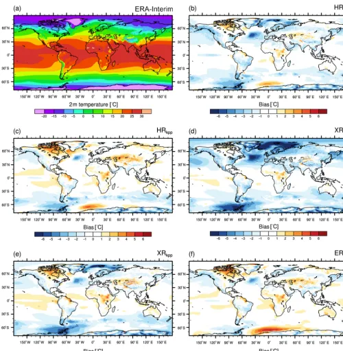
3.1.2 2 m temperature
Figure 1.Annual mean 10 m wind speed from(a)ERA-Interim (1979–2005) and the bias of(b)HRpp,(c)HRkpp,(d)XRpp,(e)XRkpp, and (f)ERpp.
the vertical ocean mixing parameterization. Over the ocean, it closely resembles the bias of the sea surface temperature (Sect. 4.1.1). Again, all models (except XRpp) agree well with ERA-Interim over the continents and over large parts of the world’s oceans, in particular over the tropical and sub-tropical oceans and in the Arctic Ocean.
Figure 2.Annual mean 2 m temperature from(a)ERA-Interim (1979–2005) and the bias of(b)HRpp,(c)HRkpp,(d)XRpp,(e)XRkpp, and (f)ERpp.
field removed the cold bias in the North Atlantic almost com-pletely. Another area of cold near-surface air temperature bi-ases is the region around the Antarctic peninsula. In contrast, all models (except XRpp) simulate a consistent warm bias over the Canadian Archipelago, central Africa, and central Asia. Although reduced in their magnitudes, all these biases remain in the higher-resolution models or when KPP is used.
Wed-dell Sea is more often covered with thicker ice (not shown), causing colder near-surface temperatures. However, a severe cold bias develops over the North Atlantic and the Nordic Seas in XRpp, as mentioned before. As a consequence, the temperatures over Europe decrease as well.
Using the KPP scheme in HR (Fig. 2c) results in warmer 2 m temperatures in the Northern Hemisphere, so cold biases are reduced, but warm biases become stronger. The reason is a stronger northward heat transport into the North Atlantic (see Sect. 4) and thus a stronger heat release to the atmo-sphere. In XRkpp(Fig. 2e), the warming caused by the KPP scheme and the cooling caused by the T255 atmosphere com-pensate for one another, so the bias pattern in the Northern Hemisphere is comparable to that of HRpp. The cold bias along the ACC, however, is not affected by KPP and is simi-lar to XRpp.
Compared to HRpp, most of the cold biases vanish in ERpp; in the region of the ACC, this is partly due to re-solved eddies and improved mean flow. The warm bias in the Weddell Sea, however, is considerably enhanced in the Atlantic sector of the Southern Ocean, because of more fre-quent open-ocean polynyas in ERpp.
3.2 Vertical structure of zonal wind speed and temperature
3.2.1 Zonal wind speed
Figure 3 shows the ERA-Interim climatology of the time-averaged zonal-mean wind speed (uvelocity) and the model biases. Overall, the vertical structure of the zonal wind speed is well represented in MPI-ESM1.2. A consistent bias in all simulations is too-strong subtropical jets (centred at ∼
200 hPa). These too-strong jets contribute further to higher zonal wind speeds extending into the upper troposphere at 40 to 45◦S and 40 to 45◦N, as also found by Müller et al. (2018). Furthermore, too-strong zonal wind speeds are sim-ulated in the troposphere in the tropics at roughly 400 hPa.
All models simulate consistently too-low zonal wind speeds over the Southern Ocean at ∼60◦S throughout the whole troposphere. The overall bias pattern in HRkpp (Fig. 3c) is very similar to HRpp(Fig. 3b), although the bias over the Southern Ocean is reduced and increases in the up-per troposphere. The T255 atmosphere in the XR models am-plifies all biases (Fig. 3d–e). That is, the subtropical jets be-come stronger and shift equatorwards, and the zonal wind speed over the Southern Ocean reduces further.
Important for the ocean is the extension of the negative bias over the Southern Ocean down to the surface in both XR simulations (stronger in XRppthan in XRkpp), which reduces the zonal wind stress driving the ACC and the upwelling of Circumpolar Deep Water (CDW). However, this wind bias in XR was found not to be the cause of the AMOC collapse (Putrasahan et al., 2019). Note that the near-surface negative
bias for the North Atlantic cannot be seen here, as discussed above, because it cancels in the zonal mean.
The bias pattern in ERpp (Fig. 3f) is similar to HRpp and HRkpp, which indicates that the ocean resolution does not have a large impact on the mean zonal wind speed. However, both the positive bias in the subtropical jet in the Northern Hemisphere and the negative bias north of 60◦N are slightly amplified.
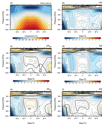
3.2.2 Zonal temperature
The cross-sections of the global time-mean zonal-mean tem-perature (Fig. 4) show cold biases in the upper troposphere (at∼250 hPa) in both hemispheres. In the HR/XR simula-tions with PP (Fig. 4b, d), the cold bias extends to the sur-face in both hemispheres (Fig. 4b, d). In HRkpp, however, this bias disappears (Fig. 4c) and emerges only weakly in XRkpp (Fig. 4e).
In XRpp, the surface-extending cold bias becomes larger in the lower troposphere compared to HRpp, because of the weaker AMOC and the freezing of the Labrador and Nordic seas (see Sect. 4 below). In contrast, the AMOC remains stable in XRkpp(Fig. 4e), so no severe cold bias evolves in the lower troposphere of the Northern Hemisphere. However, the KPP scheme does not affect the cold bias in the South-ern Hemisphere, as already found for the 2 m temperature. A clear improvement can be seen in ERpp (Fig. 4f), which removes both biases in the lower and middle troposphere in both hemispheres. We conclude that a high ocean resolution plays a major role for the mean states of the large-scale tem-perature distribution in the atmosphere. Although the large cold bias above the Antarctic continent is present in all sim-ulations, the bias is reduced in ERppby about 2◦C. The de-veloping warm bias over the Weddell Sea in ERpp can also be seen in the cross-section at roughly 60◦S.
4 Evaluation of the ocean mean state 4.1 Ocean surface temperature and salinity 4.1.1 Sea surface temperature
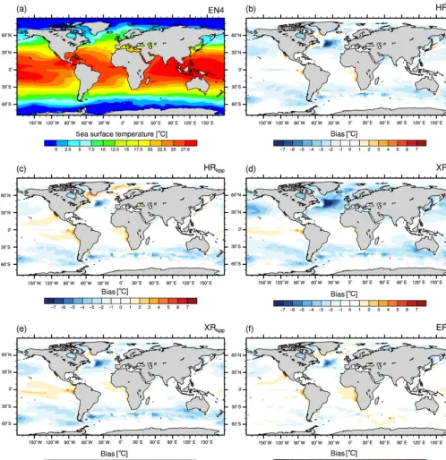
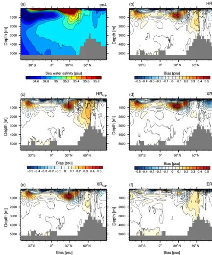
The sea surface temperature bias of MPI-ESM1.2 with re-spect to the UK Met Office EN4 data (version 4.2.0; Good et al., 2013, averaged from 1945 to 1955) is shown in Fig. 5. We used this period for EN4 since our HR simulations were initialized from a simulation that was nudged to the averaged EN4 state of 1950–1954, and we further allow for some vari-ance. The results differ only marginally if another period is chosen (not shown). In general, biases occur in prominent ar-eas and are affected by both changing the model resolution and the vertical ocean mixing scheme.
sim-Figure 3. Global zonally averaged u velocity from(a)ERA-Interim (1979–2005) and the bias (MPI-ESM1.2 minus ERA-Interim) of (b) HRpp, (c)HRkpp,(d)XRpp,(e)XRkpp, and(f)ERpp. The zero contour line is shown as a thick solid line; negative (positive) con-tours are dashed (solid).
ulated in the Northern Hemisphere by HRpp (Fig. 5b). The strongest cold bias of up to−7◦C occurs in the North At-lantic between 40 and 50◦N, centred at about 30◦W. A sim-ilar magnitude was described by Müller et al. (2018) for MPI-ESM1.2-HR. The main explanation for this cold bias, as given in Sect. 3.1.2, is a too-zonal NAC (Dengg et al.,
Figure 4.Global zonally averaged temperature from(a)ERA-Interim (1979–2005) and the bias (MPI-ESM1.2 minus ERA-Interim) of (b)HRpp,(c)HRkpp,(d)XRpp,(e)XRkpp, and(f)ERpp. The contour lines in panels(b)–(f)span±0.75 with an interval of 0.5 K, and of 1.0 K outside that range. The zero contour line is shown as a thick solid line; negative (positive) contours are dashed (solid).
Too-cold sea surface temperatures are further simulated along the ACC (bias of∼2◦C). Coastal upwelling areas west of Africa and South America are about 1 to 2◦C too warm in
all simulations with the T127 atmosphere (Fig. 5b, c, f), as found by Milinski et al. (2016)
Increasing the atmospheric resolution from T127 to T255, while using the PP scheme (XRpp), causes a severe cold bias in the whole Northern Hemisphere (Fig. 5d) and is strongest in the North Atlantic (−9◦C). This cooling was already
Figure 5.Sea surface temperature (◦C) from(a)EN4 (averaged over 1945–1955) and differences: MPI-ESM1.2 minus EN4 for(b)HRpp, (c)HRkpp,(d)XRpp,(e)XRkpp, and(f)ERpp.
AMOC due to weak wind stress over the subpolar gyre and weak northward heat and salt transport (Table 4, Fig. A1, and Sect. 4.6). Although the reduced wind stress over the South-ern Ocean (Fig. 1) might also contribute to a weakening of the AMOC (Toggweiler and Samuels, 1995) in XRpp, Pu-trasahan et al. (2019) found no effect of this negative wind bias on the AMOC slowdown, and argue that the timescale
of the slowing AMOC is much faster than any feedback from the Southern Ocean to the North Atlantic.
Fur-thermore, the Pacific cold tongue almost disappears, but now the tropical Pacific becomes too warm south of the Equator.
The cold bias in the North Atlantic diminishes drastically with the KPP scheme in HRkpp(Fig. 5c), but the warm bias in the Labrador Sea and in the Nordic Seas is enhanced because of an increased heat transport into the North Atlantic and its ambient seas (Fig. A1c). Moreover, a warm bias evolves in the tropical Pacific north and south of the Equator. How-ever, the KPP scheme simulates a stable AMOC in XRkpp (Fig. 5e), because of a stronger subpolar gyre (see Table 2). The enhanced deep convection and North Atlantic Deep Wa-ter (NADW) formation in the Labrador Sea (Sect. 4.5) sus-tains a strong enough upper cell of the AMOC (Sect. 4.6) and thus a sufficient northward transport of heat and salt (see Ta-ble 4 and Fig. A1c–d). This surplus in heat and salt transport, compared to XRpp, prevents the Labrador Sea from freezing over. This finding is an important result and provides a solu-tion to the declining AMOC strength for MPI-ESM1.2-XR. In addition, enhanced upwelling in the Southern Ocean fur-ther strengthens the norfur-thern cell of the AMOC (Marshall et al., 2017), although it is not the main reason in our model. The cold bias along the ACC is clearly reduced in ERpp (Fig. 5f), because of resolving eddies that flatten and shift the outcropping isopycnals southwards. Furthermore, the cold biases in the North Atlantic, in the North Pacific, and in the Mediterranean Sea are reduced. The warm biases in the up-welling regions, however, remain because of the coarse T127 atmosphere.
4.1.2 Sea surface salinity
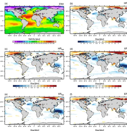
As with sea surface temperature, the sea surface salinity is well simulated by MPI-ESM1.2 for most parts of the ocean with respect to EN4 (Fig. 6). However, in some areas, we find larger discrepancies. In the North Atlantic, the surface waters are too fresh where we already found a cold bias. This fresh bias is again caused by the too-zonal NAC and the entrain-ment of fresher water masses from the Labrador Current. Al-though all models produce this bias, it is most pronounced in XRpp, likely due to a too-stable stratification in association with excessive export of salty water from the Mediterranean (compare with Figs. 8d and A6d).
The fresh bias in the North Atlantic (Fig. 6c) diminishes when using the KPP scheme or the high-resolution ocean. In both cases, a stronger northward salt transport is simu-lated in the Atlantic (Fig. A1d). In the case of ERpp, the Gulf Stream separation is better represented, which further reduces the bias in the North Atlantic (Fig. 6f). The resolved eddies further remove the fresh bias along the ACC. The wa-ter masses in the Mediwa-terranean Sea become more saline, which removes the fresh bias that the HR and XR models produce.
Increasing the atmospheric resolution from T127 to T255 enhances the fresh bias in XRpp (Fig. 6d) because of the above-described AMOC slowdown, with the consequence
that less salt is transported by the Gulf Stream and the NAC into the North Atlantic (Fig. A1c–d). In XRkpp(Fig. 6e), both effects work in opposite directions and almost balance each other, so the bias is similar to that in HRpp.
Another bias present in all simulations is a too-saline near-surface Arctic Ocean, originating from the Siberian coast that extends across the Transpolar Drift Stream but also into the Canadian basin. These too-saline waters indicate too little freshwater input from the Siberian rivers, in particularly from the Lena River (Laptev Sea). Another effect that enhances this error could be too little barotropic tidal mixing along the Arctic shelves and thus too little horizontal spreading of the river waters (Q. Wang et al., 2014).
Finally, a strong fresh bias is simulated in the western trop-ical Pacific. The KPP scheme does not ameliorate this prob-lem as the surface waters become severely fresher in both XR simulations (Fig. 6d–e). In general, all models simulate too little precipitation or too much evaporation for most parts of the globe (Fig. A2). In the western Pacific, the XR mod-els even simulate slightly less precipitation (Fig. A2d–e), so we suspect that the supply of salty waters from the east is reduced in XR, thus enhancing the fresh bias.
4.2 Ocean interior
bet-Table 2.Maximum values of barotropic stream function (gyre strengths) in Sverdrup units (Sv:=106m3s−1) simulated by MPI-ESM1.2 and from observations.
Region HRpp HRkpp XRpp XRkpp ERpp Obs. Reference
Subpolar gyre 34.6 40.6 31.0 32.1 36.6 26.0–40.0 Clark (1984), Bersch (1995), Bacon (1997),
(North Atlantic) Lherminier et al. (2007), Holliday et al. (2009)
Subtropical gyre 48.2 64.9 44.0 63.9 62.8 46.0–61.0 Johns et al. (1995) (North Atlantic)
Subtropical gyre 84.1 116.3 73.6 95.5 80.7 42.0±2.5 Imawaki et al. (2001) (North Pacific)
ter resolved, producing a more realistic circulation and water-mass transfer from the Indian Ocean into the South Atlantic, as seen in other similar studies (McClean et al., 2011; Pu-trasahan et al., 2016; Cheng et al., 2018); and (2) the eddy-induced cooling and freshening of the intermediate ocean (von Storch et al., 2016) further reduces the warm bias.
The warm bias in Fig. 7a–e stretches northward at the depth of the AAIW and shows another maximum at 30◦N that is related to the spreading of Mediterranean waters. The HR and XR models use the same TP04 ocean grid and both simulate the observed net volume transport through the Strait of Gibraltar (net inflow of about 0.04 Sv; see Table 3). The outflowing Mediterranean water is too warm and too saline in all HR and XR simulations compared to EN4 (see Figs. A5 and A6), which explains the warm and saline bias (Fig. 8a– e). The Mediterranean water is slightly more saline in HRkpp than in HRpp, so the water spreading northward along the Eu-ropean continental shelf becomes also more saline and con-tributes to saltier NADW. This enhanced flow of saline water into the subpolar gyre explains the reduced salinity bias at 40 to 50◦N at a depth of 1000–1500 m (Fig. 8c). The main spreading pathway in all HR and XR models, however, is to the southwest into the open Atlantic.
As with the warm biases, the salinity biases disappear in ERpp (Figs. 7f and 8f). A fresher water mass at intermedi-ate depth reflects a much more realistic representation of the AAIW (Fig. 8 and in detail in Fig. A8) and of the outflow of Mediterranean water. The latter is less saline and about 2 to 3◦C colder (also shown at a depth of 740 m; Figs. A5f and A6f), reducing the warm and saline bias at 30◦N. The reason for this major improvement is the better resolved bathymetry of the Strait of Gibraltar, which is 12 km wide and has a sill depth of ∼300 m in the present-day real world. In the two ocean configurations discussed in this paper, this strait is about 24 km wide with a shallowest sill depth of about 230 m in the TP6M grid, compared to about 54 km and same sill depth in TP04. Although the salinity maximum of the over-flow water is about 100 m shallower than in EN4 (not shown), ERppproduces more realistic properties of upper and inter-mediate depth water masses.
Although the Gulf Stream separates earlier from the Amer-ican coast in ERpp(not shown), its flow path is still too zonal,
such that the cold bias in the North Atlantic at around 50◦N (Fig. 7) is not removed. This indicates that a high-resolution ocean alone does not solve the cold bias at 740 m in the North Atlantic. In fact, Fig. A5f suggests that the cold bias is sub-stantially larger in ERppthan in any of the other simulations. The too-warm and saline subpolar gyre causes a warm and saline bias in the deep convection areas of the Labrador and Irminger seas, centred around 60◦N (Figs. 7, 8, and A5). The bias is larger in HRkpp because of the increased trans-port of heat and salt from the subtropical gyre into the sub-polar gyre. The bias is reduced in the XR models because of the weaker subpolar gyre and the reduced salt transport by the gyre. However, from Fig. 8d, we see that the reduced salinity is the main factor causing the reduced convection in XRpp (also supported in Fig. A1d), as described by Putrasa-han et al. (2019). Another contribution is too-warm overflow waters from the Nordic Seas, an issue that was also present in coarser MPI-ESM versions (Jungclaus et al., 2013). This warm bias of the overflow waters is mostly unaffected in ERpp.
Figure 6.Sea surface salinity (psu) from(a)EN4 (averaged over 1945–1955) and for the differences: MPI-ESM1.2 minus EN4 for(b)HRpp, (c)HRkpp,(d)XRpp,(e)XRkpp, and(f)ERpp.
reflected by strong vertical mixing in the upper layers of the Arctic Ocean (Fig. A3c).
Further, less vertical mixing in the Fram Strait can reduce the inflow of Atlantic Water into the Arctic Ocean (Zhang and Steele, 2007) and thus reduce the warm bias as in ERpp. In fact, Zhang and Steele (2007) recommend to reduce the background diffusivity to 1×10⁻⁶m2s−1 and viscosity to
Figure 7.Zonal-mean temperature transect through the Atlantic basin and the Arctic Ocean of(a)EN4 (averaged over 1945–1955) and the bias (MPI-ESM1.2 minus EN4) of(b)HRpp,(c)HRkpp,(d)XRpp,(e)XRkpp, and(f)ERpp. Contour levels(b–f)begin with±0.5◦C.
Ocean removes the warm and saline bias in the Atlantic Wa-ter layer, without changing any background values for verti-cal mixing. The benefit of a very high resolution for the Arc-tic Ocean was recently demonstrated by Wang et al. (2018), who used a background diffusivity of 1×10⁻⁵m2s−1, which is close to what we chose.
4.3 Ocean circulation
Figure 8.Zonal mean salinity transect through the Atlantic basin and the Arctic Ocean of(a)EN4 (averaged over 1945–1955) and the bias (MPI-ESM1.2 minus EN4)(b)HRkpp,(c)XRpp,(d)XRkpp,(e)XRkpp, and(f)ERpp. Contour levels(b–f)begin with±0.05 psu.
to T255 reduces the gyre strengths, (2) the KPP scheme en-hances the strength of all gyres, and (3) the effect of a high-resolution ocean is bidirectional.
The simulated subpolar gyre strengths in the North At-lantic range from 31.0 to 0.6 Sv and are all within the obser-vational range of 26.0 to 40.0 Sv (Table 2). HRkppsimulates a
stronger subpolar gyre (+6 Sv) than the reference simulation HRpp. Both XRpp and XRkpp show weaker gyres compared to their respective HR counterpart, whereas ERppsimulates a slight increase of the gyre strength.
ver-Table 3.Simulated (mean±1 standard deviation) and observed net volume transport (Sv:=106m3s−1) across sections (positive means northward).
Section HRpp HRkpp XRpp XRkpp ERpp Obs. Reference
Bering Strait 0.7±0.1 0.7±0.1 0.5±0.1 0.6±0.1 0.9±0.1 0.8 [0.7–1.1] Woodgate et al. (2006, 2012)
Fram Strait −2.5±0.6 −1.9±0.4 −2.5±0.6 −1.9±0.5 −1.0±0.4 −1.75±5.01 Fieg et al. (2010)
Denmark Strait −3.9±0.6 −4.2±0.7 −4.1±0.6 −3.9±0.7 −4.6±0.4 −4.6 Hansen et al. (2008) −3.4±1.4 Jochumsen et al. (2012) −3.2±0.5 Jochumsen et al. (2017)
Iceland–Scotland 4.0±0.8 5.0±1.0 4.2±0.8 4.4±1.0 5.5±0.6 4.8 Hansen et al. (2008) 4.6±0.25 Rossby and Flagg (2012)
3.8±0.6 Kanzow and Zenk (2014)
Florida Current 14.6±0.7 15.5±0.7 12.4±0.6 14.1±0.6 24.7±0.8 31.7 Kanzow et al. (2010) 31.6±2.7 McDonagh et al. (2015)
Strait of Gibraltar 0.04±0.01 0.04±0.01 0.04±0.01 0.04±0.01 0.05±0.01 0.038±0.007 Soto-Navarro et al. (2010) 0.041 Bryden et al. (1994)
Indonesian 8.5±0.8 9.5±0.9 8.0±0.5 8.5±0.8 13.0±0.8 11.6 to 15.7 Gordon et al. (2010) Throughflow
Mozambique 8.8±1.7 6.5±2.0 8.0±1.3 5.3±1.9 13.6±1.2 5.0 to 26.0 DiMarco et al. (2002)
Channel 16.7±8.9 Ridderinkhof et al. (2010)
Drake Passage 161.7±3.0 191.9±2.6 150.1±4.1 170.2±3.0 140.9±3.0 134.0±14.0 Nowlin and Klinck (1986) 137.0±8.0 Cunningham et al. (2003) 136.7±6.9 Meredith et al. (2011) 173.3±10.7 Donohue et al. (2016)
Table 4.Time-mean AMOC volume transport (±1 standard deviation of annual means) at 26◦N in 1000 m depth simulated by MPI-ESM1.2 and the depth of the North Atlantic Deep Water (NADW) cell at 26.5◦N (defined where the stream function crosses zero). The observed annual mean (±1 standard deviation) NADW cell depth from the RAPID-MOCHA-WBTS array (Smeed et al., 2017) is 4379±279 m. Further, the time-mean (±1 standard deviation of annual means) heat and salt transport across 50◦N is shown (positive means northward transport).
Property HRpp HRkpp XRpp XRkpp ERpp
AMOC volume (Sv) 14.9±3.5 18.9±4.0 11.0±3.8 14.6±3.9 14.9±3.6
NADW cell depth (m) 2865±270 3176±334 2665±287 2979±489 2941±265 Atl. heat transport across 50◦N (PW) 0.60±0.04 0.63±0.06 0.42±0.06 0.52±0.05 0.57±0.03 Atl. salt transport across 50◦N (106kg s−1) 0.28±1.89 0.64±2.18 −1.04±2.54 0.4±2.11 −0.22±1.27
tical ocean mixing scheme and to resolving of ocean ed-dies. Compared to the reference of 48.2 Sv (HRpp), the gyre strength decreases slightly to 44.0 Sv with a higher atmo-spheric resolution (XRpp). By using the KPP scheme, how-ever, the gyre strength increases to 64.9 Sv (HRkpp) and re-mains similarly high with a T255 atmosphere (XRkpp). ERpp produces a gyre strength as strong as with the KPP scheme. With that, the strength of the North Atlantic subtropical gyre of the KPP and ER simulations slightly exceeds the bound of the observed range, while that of the PP simulations hov-ers around the other end of the observed range. In the case of HRkppand XRkpp, the too-strong volume transport of the subtropical gyre might further contribute to the positive salin-ity bias in the subpolar gyre at a depth of 500 to 1000 m
(Figs. 8 and A6). The results for the subtropical gyre of the North Pacific reveal a similar picture as in the North Atlantic with stronger transport in the KPP simulations. One excep-tion is a markedly reduced gyre strength in ERpp. Further-more, all simulations produce a considerably stronger North Pacific gyre than what has been derived from observations.
outflow of Mediterranean water through Strait of Gibraltar in ERpp, this improvement is due to a better resolved Bering Strait.
The simulated net transport through the Fram Strait is in the range of the observations (−1.75±5.01 Sv), which show a strong interannual variability (Fieg et al., 2010). A possi-ble explanation for the somewhat lower transport with KPP is given by Zhang and Steele (2007). They found that strong vertical mixing, as with the KPP scheme in our HR and XR simulations, deepens the Atlantic Water layer but simultane-ously weakens the inflow of Atlantic Water and the outflow of Arctic Water.
In our KPP simulations, the outflow becomes weaker com-pared to the PP simulations, whereas the inflow is of similar magnitude, so the net transport is lower. However, in compar-ison to the HR and XR simulations, the net transport in ERpp is only half on average. In agreement with Fieg et al. (2010), the West Spitsbergen Current (WSC) is better resolved in ERpp. The WSC, and thus the inflow of Atlantic Water into the Arctic Ocean, is much stronger in ERpp, as is its re-turn circulation north of 80◦N. This intensified WSC and its recirculation cause a reduction of the net volume transport through the Fram Strait. Considering the high uncertainty of the net transport from observations, all simulations give real-istic estimates, but the most realreal-istic simulation with respect to the temperature and salinity structure and to the circulation is ERpp(not shown).
The overflows through the Denmark Strait and across the Iceland–Scotland ridge are important deep water connections for the Arctic and the Atlantic. All simulations produce real-istic overflow volumes with respect to observations, which are on average slightly higher in ERpp but still within the standard deviation of the coarser simulations. The higher transport in HRkppvs. HRppis caused by enhanced deep con-vection in the Nordic Seas, particularly in the Greenland Sea (Fig. 10).
In all HR and XR simulations, the volume transport of the Florida Current is only about half the observed value of roughly 32 Sv (Table 3). Although the transport increases with the KPP scheme, only ERpp simulates a considerably (about 10 Sv) stronger transport, amounting to about 25 Sv. We found similar results for the Indonesian Throughflow, which is important for climate because it connects the Pacific with the Indian Ocean and closes the upper warm branch of the meridional overturning circulation (MOC). Again, KPP enhances the transport slightly, but only ERpp simulates a transport strength that is similar to observed values.
The Mozambique Channel is an example where both a T255 atmosphere and KPP show a reduction in the transport. In ERpp, however, the transport is about twice as high as in the other simulations and more realistic with respect to recent observations of 16.7±8.9 Sv (Ridderinkhof et al., 2010). The ability to resolve eddies, particularly the Mozambique eddies along with a better resolved southward advection through the Mozambique Channel, contributes to the more realistic
trans-port of about 14 Sv in ERpp (Putrasahan et al., 2016; Rid-derinkhof et al., 2010).
The observed baroclinic transport through the Drake Pas-sage was commonly estimated at roughly 140 Sv. However, a new estimate reveals a much higher transport volume of about 173.3±10.7 Sv, when adding the barotropic transport (Donohue et al., 2016). With regard to this estimate, the models are within or close to the observed range. However, compared to the reference simulation (HRpp) (161.1 Sv), the transport weakens to about 150.0 Sv in XRpp, and from 191.9 Sv in HRkppto 170.3 Sv in XRkpp. In ERpp, the trans-port is lower than in all other simulations (about 141 Sv). These results confirm that a higher atmospheric or ocean res-olution reduces the transport in the Drake Passage, consis-tent with what has been found Stössel et al. (2015). In con-trast, the transport through the Drake Passage is enhanced when using the KPP scheme, probably because of enhanced deep convection in the Weddell Sea (Fig. 11) that steep-ens the isopycnals across the ACC and thus increases the geostrophic flow (Stössel et al., 2015; Naughten et al., 2018) (see Sect. 4.5.2).
4.4 Sea ice
4.4.1 Arctic Ocean
Figure 9.Time-averaged Arctic sea ice thickness in March for(a)the Pan-Arctic Ice-Ocean Modeling and Assimilation System (PIOMAS) reanalysis (Zhang and Rothrock, 2003),(b)HRpp,(c)HRkpp,(d)XRpp,(e)XRkpp, and(f)ERpp. Simulations include their 15 % sea ice concentration contour in magenta and all figures include the EUMETSAT OSI SAF observed ice edge (15 % contour) in dark blue (averaged March 1979–2005).
reaches Iceland as in the reference simulation. Compared to HRpp, the sea ice thickness of HRkppis slightly lower in the Eurasian basin, although it becomes thicker in the Canadian basin. XRpp(Fig. 9c) simulates more, although thin, sea ice in the Labrador Sea because of the above-described fresher and colder North Atlantic and the resulting freeze-over. The sea ice cover in the Iceland Sea reaches even further south than in the reference simulation HRpp. In contrast, in XRkpp (Fig. 9d), the ice thickness and extent in the Labrador Sea are similar to those in HRpp. However, due to colder sea surface temperatures in the Denmark and Fram straits than in HRkpp, a southern tongue of sea ice extends to Iceland as in HRpp. Further, in contrast to HRkpp, the recirculating branch of the West Spitsbergen Current does not become stronger in the XR simulations (not shown).
In addition, the near-surface circulation in the Arctic Ocean changes with a T255 atmosphere from a more anti-cyclonic circulation in the Makarov and Canadian basins in HR, to a more cyclonic circulation in XR (not shown). A cy-clonic circulation enhances the export of cold Arctic Water via the East Greenland Current, causing colder sea surface temperatures in the Nordic Seas. The XR simulations and ERppproduce thinner winter ice in the Canadian basin, which may be related to the changed circulation but has to be fur-ther investigated. ERppproduces in general a much lower sea ice volume the Arctic Ocean than the HR/XR simulations.
at-mosphere. KPP again simulates thinner ice in the Canadian basin (about−0.5 m).
4.4.2 Southern Ocean
The spatial distribution of austral winter (September) sea ice thickness in the Southern Ocean of HRpp (not shown) is similar to the MPI-ESM1.2-HR simulations described by Müller et al. (2018). The ER and both HR simulations pro-duce an overabundance of open-ocean polynyas in the Wed-dell Sea (see Sect. 4.5.2). HRkppsimulates less and thinner ice in the Weddell Sea than HRpp, but otherwise the spatial distribution of sea ice in the Southern Ocean is very similar.
Both XR simulations, but more so XRpp, produce thicker sea ice than the other simulations, in particular in the Wed-dell Sea and close to Antarctica’s coasts. The thicker ice in the Weddell Sea emerges in concert with a reduced number of polynyas, so the warm bias seen in Fig. 2 vanishes. This less frequent occurrence of Weddell Sea polynyas is proba-bly related to a reduced meridional pressure gradient across the Weddell Sea and the ACC (not shown), which in turn re-duces the near-surface wind speed bias (as seen in Fig. 1). However, a more detailed investigation is required to explain circulation differences between the T127 and the T255 atmo-spheres over the Weddell Sea. In austral summer, both XR models produce thicker ice in the Weddell Sea (not shown), so the ocean is insulated from the cold atmosphere above, resulting in less convective mixing.
4.5 Mixed layer depth and diapycnal mixing 4.5.1 Northern Hemisphere
Figure 10 shows the average mixed layer depths in March for the northern North Atlantic. We diagnosed the mixed layer depth as the depth where the density deviates from the sur-face density byσt=0.01 kg m−3. This diagnostic was com-puted from monthly means. As with observations, we use the mixed layer depth retrieved from Argo floats by the den-sity threshold method (σt=0.03 kg m−3) from the gridded 1◦×1◦monthly climatology (January 2000 to April 2018) from Holte et al. (2017). We interpolated the Argo mixed layer depths onto the TP04 grid. Missing values were filled by the nearest non-missing neighbour, and values south of 60◦S and north of 80◦N were discarded and masked because of the sparseness of Argo data below sea ice.
In the reference simulation, HRpp(Fig. 10b), March-mean depths of up to 1500 m are simulated in the Labrador Sea, which is deeper than the observed 1200 m in March from Argo (Fig. 10a). The area with deep mixed layers wraps around southern Greenland with depths up to 1000 m south of Cape Farewell, in the Irminger Sea, and in the Nordic Seas. In the Irminger Sea, HRppsimulates too-shallow mixed lay-ers of only about 500 m depth. Similarly, too-shallow mixed layers are simulated in the Greenland Sea.
As discussed before, in XRpp(Fig. 10d), the deep convec-tion in the Labrador Sea ceases within the first two decades of the simulation. This collapse of deep convection (together with that in the Nordic Seas) leads to a slowing down of the AMOC (Table 4) (Putrasahan et al., 2019).
The KPP scheme in HRkpp(Fig. 10c) causes much deeper mixed layers in the Labrador Sea and in the Greenland Sea. In particular, the mixed layer depths in the Labrador and Irminger seas and south of Greenland (north of 50◦N) be-come deeper compared to all other simulations. These deeper mixed layers with the KPP scheme result on one hand from the convection parameterization (i.e. the non-local fluxes) and on the other hand from a stronger and more cyclonic subpolar gyre (Table 2) that domes the isopycnals in the gyre centres (not shown), which preconditions the water col-umn for convection. As mentioned in Sect. 2.2, the non-local fluxes in the KPP scheme have the same vertical diffusivi-ties as those for the local gradient transport. These diffusiv-ities are not limited to a user-defined maximum value dur-ing convective forcdur-ing conditions, so much larger diffusivi-ties can act to redistribute temperature and salinity through-out the ocean water column, causing it to overturn faster and to produce deeper mixed layers with the KPP than with the PP scheme. We speculate that the non-local transport terms in KPP cause a more efficient convection than the enhanced wind-mixing parameterization of our PP scheme. The diffu-sivity in KPP is further enhanced as it also depends on the mixed layer depth, which reflects that boundary layer eddies become larger with deeper mixed layers.
On the other hand, XRkpp(Fig. 10e) simulates shallower mixed layers compared with HRkpp. These shallower mixed layers result from the reduced wind stress of the T255 at-mosphere by means of two processes: (1) less positive wind stress curl spins down the subpolar gyre, so the slower cy-clonic circulation reduces the isopycnal doming and the hor-izontal salt advection to the gyre centres (Table 4), leading to a more stratified surface layer; and (2) lower near-surface wind speeds reduce the turbulent air–sea fluxes via the bulk formula and the surface friction velocity (u∗). Lesser heat
fluxes in turn reduce directly the non-local fluxes of the KPP scheme in convection areas, and loweru∗reduces the
turbu-lent vertical velocity scales, which results in lower vertical diffusivities and viscosities.
Based on these results, increasing the atmospheric resolu-tion reduces the mixed layer depths over the North Atlantic and the Nordic Seas, whereas KPP deepens them. By com-bining both the T255 atmosphere and the KPP scheme, the above effects compensate for each other (XRkpp; Fig. 10e). In contrast to XRpp, where the convection ceases in the Labrador and GIN seas, the combination of T255 and KPP (XRkpp) produces more realistic mixed layers depths even with reduced wind stress.
Figure 10.Time-averaged mixed layer depth (σt=0.01 kg m−3) in March in the North Atlantic and the Nordic Seas from(a)1◦×1◦gridded Argo float data (Holte et al., 2017) and from(b)HRpp,(c)HRkpp,(d)XRpp,(e)XRkpp, and(f)ERpp.
Labrador Sea, Irminger Sea, and Nordic Seas. For this rea-son, HRkpp simulates enhanced deep convection compared with HRpp, in particular in the Labrador and GIN seas. In the Irminger Sea, mixed layer depths of about 400 to 500 m are simulated by both HRkppand XRkpp, which is consistent with retrievals from observations (e.g. Pickart et al., 2003; Våge et al., 2008, 2011), although too shallow compared to Argo (Fig. 10a). One explanation for these too-shallow mixed layers is that even the T255 atmosphere is too coarse to fully simulate Greenland tip jets (e.g. Martin and Moore, 2007; DuVivier and Cassano, 2016; Gutjahr and Heinemann, 2018). The tip jets have a considerable impact on triggering deep convection in the Irminger Sea due to strong associ-ated wind stress curls driving the Irminger Gyre, and turbu-lent fluxes of heat and momentum removing the near-surface stratification. Because of the unresolved tip jets, the mixed layer depth may be underestimated in winters with high tip jet activity.
The mixed layer depths in the Labrador Sea are neverthe-less too deep (excluding XRpp). A possible explanation is the neglect of tidal mixing in MPI-ESM1.2. As shown by Müller et al. (2010), tidal mixing improves the recirculation of the Labrador Current. By entraining more freshwater into the surface layer of the Labrador Sea, it becomes more stratified, which in turn reduces deep convection. Another shortcoming is probably insufficient eddy activity in the Labrador Sea, so too little freshwater is transported from the West Greenland
Current into the interior of the Labrador Sea (e.g. Eden and Böning, 2002; Kawasaki and Hasumi, 2014).
In ERpp (Fig. 10f), the mixed layer depths are to a large extent similar to our reference simulation (HRpp). However, the convection centre in the Labrador Sea is confined to a more southeastern area with deeper mixed layers in ERpp. This is due to resolved eddies, in particular Irminger Rings, that flatten the isopycnals, thereby limiting the northward ex-tent of the convection area (Rieck et al., 2019). The resolved eddy activity can be seen in the eddy kinetic energy field (Fig. A9), defined as EKE=1
2(u02+v02)in m
2s−2, where (u0, v0=u−u, v−v) with (u, v) the monthly mean zonal and meridional velocity. The EKE shows the largest values origi-nating in the West Greenland Current and eddy shedding into the inner Labrador Sea. These eddies confine deeper mixed layers to the area with minimum EKE. However, a resolution of 0.1◦is still not sufficient to resolve so-called convective eddies, which emerge from baroclinic instabilities at the rim of the mixed patch due to strong buoyancy gradients and are thought to be the main process for rapid restratification in spring (Rieck et al., 2019).
An-other reason could be enhanced advection of Labrador Sea water from the Labrador into the Irminger basin that pre-conditions the water south of Cape Farewell for convection. However, the processes that lead to deep convection in the Irminger Sea are complex, and it is still not fully understood how eddies affect the preconditioning/triggering of convec-tion and where their main formaconvec-tion area is (Fan et al., 2013; DuVivier and Cassano, 2016).
4.5.2 Southern Hemisphere
In the Southern Ocean, we define the mixed layer depth as the depth where the density deviates byσt=0.03 kg m−3from the surface. MPI-ESM1.2 simulates very deep winter mixed layers in the Weddell and Ross seas (Fig. 11). The main rea-sons for the mismatch with mixed layer depths derived from Argo floats is the lack of such floats in ice-covered regions, even though some under-ice float data have recently become available (e.g. Campbell et al., 2019). In the Weddell Sea, the convection reaches down into the deep ocean, which is a known problem in many state-of-the-art ESMs (Sallée et al., 2013; Kjellsson et al., 2015; Heuzé et al., 2015; Naughten et al., 2018). Spurious open-ocean deep convection leads to semi-permanent Weddell Sea polynyas, as warm Circumpo-lar Deep Water is continuously brought to the surface, caus-ing sea ice to melt so that the ocean becomes exposed to the cold atmosphere.
Possible explanations for this widespread bias are insuf-ficient freshwater input (Kjellsson et al., 2015), in particu-lar glacial meltwater (e.g. Stössel et al., 2015), and insuffi-cient wind mixing in summer (Timmermann and Beckmann, 2004). Reduced wind mixing allows salt from brine rejec-tion to accumulate in the winter water layer and eventually to erode the stratification. In both cases, salinity increases in the winter upper layer until the weakly stratified water col-umn overturns (Naughten et al., 2018).
The diagnosed mixed layer depth, however, is very sen-sitive to the chosen density threshold because of the very weakly stratified water column. We decided to apply a commonly used threshold for the Southern Ocean of σt= 0.03 kg m−3, but note, however, that if a lower threshold of σt=0.01 kg m−3is chosen, the mixed layer depth rarely ex-ceeds 300 m, because of a shallow stratified surface layer.
Based on two simulations with the Geophysical Fluid Dynamics Laboratory Earth system model (GFDL-ESM) with different resolutions of their ocean component (0.25 and 0.1◦), Dufour et al. (2017) found that deep
convec-tion in the Weddell Sea does not necessarily lead to open-ocean polynyas. They argue that excessive vertical mixing in the lower-resolution ocean component hinders the build-up of a heat reservoir at depth that is necessary for Wed-dell Sea polynyas to occur intermittently as expected under pre-industrial conditions (e.g. de Lavergne et al., 2014; Gor-don, 2014). They further argue that the more realistic rep-resentation in the higher-resolution simulation stems from
(1) the fact that mesoscale eddies tend to flatten isopycnals, thereby increasing the stratification, and (2) the more detailed bathymetry which allows for a better simulation of dense-water overflows.
Based on forced MPIOM and coupled MPI-ESM simu-lations with varying resolution, Stössel et al. (2015) found that the Southern Ocean winter sea ice and water properties of a 0.1◦ (TP6M) ocean simulation improved considerably upon switching from a forced to a coupled mode of opera-tion, largely due to an associated increase in surface fresh-water flux. These findings are consistent with our ERpp sim-ulation (Fig. 11f), where the mixed layer depth in the cen-tral Weddell Sea is overall reduced in comparison with HRpp (Fig. 11b). At the same time, the area of deep mixed lay-ers shifts to the eastern part of the Weddell Sea, close to the Maud Rise plateau, where ERppstill simulates very deep mixed layers in September. This, in turn, could be a result of the better resolved bathymetry in this region. Kurtakoti et al. (2018) explained how Maud Rise polynyas formed in a high-resolution (0.1◦ ocean component) ESM simulation, while none formed in a low-resolution simulation with the same model. A decisive reason for this was the steeper and better resolved bathymetry of and around Maud Rise that allowed for sufficiently strong Taylor columns to form.
For the larger Weddell Sea polynyas, de Lavergne et al. (2014) and Gordon (2014) argue that such should only emerge under pre-industrial conditions. Even though de Lavergne et al. (2014) praise the low-resolution MPI-ESM for belonging to the class of convecting models, Kurtakoti et al. (2018) explain that large-scale Weddell Sea polynyas should only occur intermittently under pre-industrial condi-tions and only by growing out from Maud Rise polynyas, which themselves should only occur at high model resolu-tion (0.1◦). Since the greenhouse gas forcing of the experi-ments presented here is fixed at the 1950 level, one would expect the Southern Ocean of the model to already have adjusted to the present-day situation when no Weddell Sea polynyas are expected to occur (due to the southward shift of the precipitation-rich westerlies). Strong convection and large Weddell Sea polynyas, as implied by the perpetual large regions of excessively deep mixed layers (Fig. 11), should thus be viewed as an unrealistic behaviour.
Figure 11.Time-averaged mixed layer depth (σt=0.03 kg m−3) in September in the Southern Ocean from(a)1◦×1◦gridded Argo float data (Holte et al., 2017) and from(b)HRpp,(c)HRkpp,(d)XRpp,(e)XRkpp, and(f)ERpp.
convection contributes to the enhanced ACC strength (Ta-ble 3), as it causes a steepening of the isopycnals across the ACC and thus an increased geostrophic flow (Jungclaus et al., 2013; Stössel et al., 2015; Naughten et al., 2018). This is another indication that the eddy activity is too low in the KPP simulations, so isopycnals remain too steep and the wa-ter too weakly stratified.
Besides the resolution of the ocean component and the choice of the vertical ocean mixing scheme, a higher reso-lution of the atmosphere component has also a distinct ef-fect on the simulated winter mixed layer depth (Fig. 11d vs. Fig. 11b and Fig. 11e vs. Fig. 11c), which is related to the reduced meridional pressure gradient (not shown) over the Weddell Sea. Stössel et al. (2015) found an improvement of the high-latitude Southern Ocean water-mass properties and winter sea ice cover in a simulation, where the high-resolution (TP6M) MPIOM was coupled to a T255
atmo-sphere (ECHAM6) compared to a coupled simulation with a TP6M ocean and T63 atmosphere. In terms of the ocean mixed layer depth, our results support these earlier findings, as also indicated by the reduction of the ACC to more realis-tic values (Table 3).
Another modelling challenge is the mixed layer depth in the Subantarctic frontal zone equatorwards of the ACC (Rin-toul and Trull, 2001). This is an important area for heat and CO2uptake and for the formation of the Subantarctic Mode Water. State-of-the-art ocean models simulate very shallow mixed layers between 40 and 60◦S in comparison to Argo float observations (DuVivier et al., 2018). This discrepancy is in particular large in September when the Argo float data consistently show mixed layer depths of about 400 m (see Fig. 2 in DuVivier et al., 2018 and Fig. A10), even reaching depths of 700 m (Holte et al., 2017). Low-resolution mod-els (e.g. 1◦), however, simulate depths of only 200 to 300 m (DuVivier et al., 2018).
The main reason is that the ocean boundary layer in the models is not penetrating deep enough into the stratified sub-surface ocean, where a high salinity maximum layer is ob-served between 150 and 200 m depth that originates from the Agulhas retroflection. This layer is modified in a com-plex way by Ekman pumping/suction. This subsurface salin-ity maximum builds up over spring and early summer and is mixed out in September. It is expected that the mixed layer depths increase by either increasing the horizontal resolution or by improving the vertical mixing parameterizations (Du-Vivier et al., 2018), allowing deeper penetrations of the ocean boundary layer into the subsurface salinity core.
The Argo data (Fig. A10a) show mixed layer depths in excess of 400 m in the deep mixing band. Our reference sim-ulation (HRpp) simulates too-shallow mixed layers of only about 200 to 300 m (Fig. A10b), which is in agreement with the results from DuVivier et al. (2018). Deeper mixed lay-ers are simulated by either using the KPP scheme (HRkpp; Fig. A10c) or by increasing the ocean resolution (ERpp; Fig. A10f). Deeper mixed layers as in ERppwere also found in other eddy-resolving ocean models (R. Justin Small, per-sonal communication, 2019; Lee et al., 2011; Li and Lee, 2017). However, the reason for improved mixed layer depth with high resolution is still unclear and may be due to changes in circulation and local stratification, or indirectly due to mixing (Lee et al., 2011; Li and Lee, 2017; DuVivier et al., 2018). As already suspected by DuVivier et al. (2018), the non-local transport terms of the KPP scheme seem to favour deeper penetrations of the boundary layer into the salinity maximum layer, although this seems to happen in too wide a latitude band.
In ERpp, the deep mixed layers are sharply confined to the observed latitudinal band between 40 and 60◦S. How-ever, they appear to be deeper compared to the Argo float retrievals from Holte et al. (2017) (Fig. A10a) for reasons that need to be further investigated. Nevertheless, the simula-tion of deeper mixed layers seems to be more realistic, which gives fidelity to our models with either an eddy-resolving res-olution in the Southern Ocean or using KPP.
4.6 Atlantic meridional overturning circulation
The large-scale global MOC is an important carrier of heat and freshwater in the climate system. The AMOC is con-sidered to be the strongest part of the MOC (Trenberth and Caron, 2001). The North Atlantic contributes about 25 % of the total poleward heat flux (ocean plus atmosphere) (Srokosz and Bryden, 2015; Lozier et al., 2017). The merid-ional transport of heat and salt follows the zonally inte-grated volume transport that, when facing west, emerges a clockwise-rotating NADW cell and a anticlockwise-rotating Antarctic Bottom Water (AABW) cell.
Figure 12 shows the associated meridional overturning volume transport stream function, or AMOC, of all five sim-ulations, and Table 4 shows the time-mean AMOC strength at 26◦N at 1000 m depth, as well as the heat and salt trans-port across 50◦N. The time mean of the AMOC is about
14.9 Sv in HRpp and comparable to the 16 Sv of the MPI-ESM1.2-HR described by Müller et al. (2018). It is slightly lower than the observed mean value (±1 standard devia-tion) of 17±4.4 Sv (April 2004 to February 2017) from the RAPID array (McCarthy et al., 2015; Smeed et al., 2017). HRkpp simulates a stronger AMOC of 18.9 Sv, which is the largest value of all our simulations. A possible explanation for this is that the volume transport of the overflow waters across the Greenland–Scotland Ridge is also slightly higher with the KPP scheme (Table 3). After the overflow waters de-scend along the continental slopes and mix with ambient wa-ter masses, they contribute to a stronger NADW cell (Dick-son and Brown, 1994) in the KPP simulations.
Figure 12f shows vertical profiles of the AMOC at 26.5◦N in comparison to the RAPID data. All simulations (except XRpp) produce transport close to the observations. The vol-ume transport of HRkpp, however, is on the stronger side of the observations, whereas the transport of the other simu-lations is on the lower side of the observations. All mod-els show a too-strong southward transport of NADW below 2000 m, which suggests a too-strong Deep Western Bound-ary Current.
The reduced wind stress from ECHAM6.3 at T255 results in the above-mentioned slowdown of the AMOC in XRpp. In this simulation, the NADW cell reaches a maximum vol-ume transport of only about 11.0 Sv, which is slightly higher than the 9.0 Sv reported by Putrasahan et al. (2019). This dis-crepancy is because we analyse an earlier period of the same XRpp simulation when the AMOC is still drifting to lower values. An important finding is that XRkpp simulates a sta-ble AMOC (14.6 Sv), despite the weak wind stress with the T255 atmosphere. In terms of volume transport, going to an eddy-resolving ocean resolution (ERpp) does not increase the strength of the NADW cell. This finding is opposite to what Hewitt et al. (2016) and Storkey et al. (2018) found.
Figure 12.Eulerian stream function (Sv:=106m3s−1) of the AMOC for(a)HRpp,(b)HRkpp,(c)XRpp,(d)XRkpp, and(e)ERpp. The zero contour is drawn as a thicker line. In panel(f), annual mean profiles of the AMOC at 26.5◦N are shown as observed from April 2004 to February 2017 by the RAPID-MOCHA-WBTS array (±1 standard deviation marked by grey shading) (Smeed et al., 2017) and simulated by MPI-ESM1.2.
transport acts to flatten the outcropping isopycnals in the Southern Ocean. So eddies counteract a wind-induced steep-ening of isopycnals, while at the same time, a stronger ver-tical gradient between the AABW and the warmer ambient ocean is maintained. The flatter isopycnals reduce the ver-tical mixing because of a more stratified water column, as indicated by the reduced mixed layer depths in the Weddell Sea in ER (Fig. 11e). Reduced convection maintains denser AABW, seen by sharper gradients of temperature and salin-ity in ER (Fig. A4e), and it theoretically helps to build up a
deep heat reservoir (Dufour et al., 2017) that is required for intermittent Weddell Sea polynyas. However, in our ER sim-ulation, Weddell Sea polynyas still form too frequently. On the other hand, better resolved bathymetry is important for the formation of AABW over the continental shelves, which is partly resolved in ER.