https://doi.org/10.5194/gmd-12-3149-2019 © Author(s) 2019. This work is distributed under the Creative Commons Attribution 4.0 License.
The DeepMIP contribution to PMIP4: methodologies for selection,
compilation and analysis of latest Paleocene and early Eocene
climate proxy data, incorporating version 0.1 of
the DeepMIP database
Christopher J. Hollis1, Tom Dunkley Jones2, Eleni Anagnostou3,4, Peter K. Bijl5, Margot J. Cramwinckel5, Ying Cui6, Gerald R. Dickens7, Kirsty M. Edgar2, Yvette Eley2, David Evans8, Gavin L. Foster3, Joost Frieling5,
Gordon N. Inglis9, Elizabeth M. Kennedy1, Reinhard Kozdon10, Vittoria Lauretano9, Caroline H. Lear11, Kate Littler12, Lucas Lourens5, A. Nele Meckler13, B. David A. Naafs9, Heiko Pälike14, Richard D. Pancost9, Paul N. Pearson11, Ursula Röhl14, Dana L. Royer15, Ulrich Salzmann16, Brian A. Schubert17, Hannu Seebeck1, Appy Sluijs5, Robert P. Speijer18, Peter Stassen18, Jessica Tierney19, Aradhna Tripati20, Bridget Wade21,
Thomas Westerhold14, Caitlyn Witkowski22, James C. Zachos23, Yi Ge Zhang24, Matthew Huber25, and
Daniel J. Lunt26
1GNS Science, Lower Hutt, New Zealand
2School of Geography, Earth and Environmental Sciences, University of Birmingham, Birmingham, UK
3Ocean and Earth Science, National Oceanography Centre Southampton, University of Southampton, Southampton, UK 4GEOMAR Helmholtz Centre for Ocean Research, Kiel, Kiel, Germany
5Department of Earth Sciences, Faculty of Geosciences, Utrecht University, Utrecht, the Netherlands 6Department of Earth and Environmental Studies, Montclair State University, Montclair, New Jersey, USA 7Department of Earth, Environmental and Planetary Sciences, Rice University, Houston, Texas, USA 8Institute of Geosciences, Goethe University Frankfurt, Frankfurt am Main, Frankfurt, Germany 9School of Chemistry & School of Earth Sciences, University of Bristol, Bristol, UK
10Lamont–Doherty Earth Observatory of Columbia University, Pallisades, New York, USA 11School of Earth and Ocean Sciences, Cardiff University, Cardiff, UK
12Camborne School of Mines & Environment and Sustainability Institute, University of Exeter, Exeter, UK 13Bjerknes Centre for Climate Research and Department of Earth Science, University of Bergen, Bergen, Norway 14MARUM – Center for Marine and Environmental Sciences, University of Bremen, Bremen, Germany
15Department of Earth & Environmental Sciences, Wesleyan University, Middletown, Connecticut, USA 16Department of Geography, Northumbria University, Newcastle, UK
17School of Geosciences, University of Louisiana at Lafayette, Louisiana, Lafayette, USA 18Department of Earth and Environmental Sciences, KU Leuven, Leuven, Belgium 19Department of Geosciences, University of Arizona, Tucson, Arizona, USA
20Department of Earth and Planetary Sciences, Institute of the Environment and Sustainability, Department of Atmospheric
and Oceanic Sciences, Center for Diverse Leadership in Science, University of California, Los Angeles, California, USA
21Department of Earth Sciences, University College London, London, UK
22Department of Marine Microbiology and Biogeochemistry (MMB), NIOZ Royal Netherlands Institute for Sea Research and
Utrecht University, Den Burg, the Netherlands
23Earth and Planetary Sciences Department, University of California, Santa Cruz, California, USA 24Department of Oceanography, Texas A&M University, College Station, Texas, USA
25Department of Earth, Atmospheric, and Planetary Sciences, Purdue University, West Lafayette, Indiana, USA 26School of Geographical Sciences, University of Bristol, Bristol, UK
Received: 10 December 2018 – Discussion started: 17 January 2019 Revised: 23 June 2019 – Accepted: 3 July 2019 – Published: 25 July 2019
Abstract. The early Eocene (56 to 48 million years ago) is inferred to have been the most recent time that Earth’s at-mospheric CO2concentrations exceeded 1000 ppm. Global
mean temperatures were also substantially warmer than those of the present day. As such, the study of early Eocene cli-mate provides insight into how a super-warm Earth system behaves and offers an opportunity to evaluate climate models under conditions of high greenhouse gas forcing. The Deep Time Model Intercomparison Project (DeepMIP) is a system-atic model–model and model–data intercomparison of three early Paleogene time slices: latest Paleocene, Paleocene– Eocene thermal maximum (PETM) and early Eocene cli-matic optimum (EECO). A previous article outlined the model experimental design for climate model simulations. In this article, we outline the methodologies to be used for the compilation and analysis of climate proxy data, primarily proxies for temperature and CO2. This paper establishes the
protocols for a concerted and coordinated effort to compile the climate proxy records across a wide geographic range. The resulting climate “atlas” will be used to constrain and evaluate climate models for the three selected time intervals and provide insights into the mechanisms that control these warm climate states. We provide version 0.1 of this database, in anticipation that this will be expanded in subsequent pub-lications.
1 Introduction
Over much of the last 100 million years of Earth’s history, greenhouse gas levels and global temperatures were higher than those of the present day (Zachos et al., 2008; Foster et al., 2017). Because greenhouse gas levels are currently well above anything experienced during the modern natural cli-mate state, ancient clicli-mate archives hold important clues to our possible future climate (IPCC, 2013). This is particu-larly true for those past times when climate was consider-ably warmer and greenhouse gas levels considerconsider-ably higher than those of the present day. For instance, such intervals can provide information about the sensitivity of the climate to greenhouse gas forcing (e.g., Rohling et al., 2012; Zeebe, 2013; Caballero and Huber, 2013; Anagnostou et al., 2016) or reveal the behavior of carbon cycle feedbacks under super-warm climate states (e.g., Carmichael et al., 2017). These times of past warmth also provide a powerful means to test the outputs of climate models because they represent actual realizations of how the Earth system functions under condi-tions of greenhouse forcing comparable to the coming cen-tury and beyond. If the models can match the geological evidence of the prevailing climatic conditions, we can have
greater confidence in their skill in predicting our future cli-mate. Similarly, differences between models and data could indicate aspects of models and/or data that require further development.
This is the rationale behind DeepMIP – the Deep-time Model Intercomparison Project (https://www.deepmip.org/, last access: 30 June 2019) – which brings together climate modelers and paleoclimatologists from a wide range of disci-plines in a coordinated, international effort to improve under-standing of the climate of these time intervals, to improve the skill of climate models, and to improve the accuracy and pre-cision of climate proxies. The term “deep-time” as applied here refers to the history of Earth prior to the Pliocene, or be-fore 5 million years ago (Ma). DeepMIP is a working group in the wider Paleoclimate Modelling Intercomparison Project (PMIP4), which itself is a part of the sixth phase of the Cou-pled Model Intercomparison Project (CMIP6). In DeepMIP, we focus on three warm greenhouse time periods in the latest Paleocene and early Eocene (∼57–48 Ma), and for the first time, carry out formal coordinated model–model and model– proxy intercomparisons.
We previously have outlined the model experimental de-sign of this project (Lunt et al., 2017). Here we outline the recommended methodologies for selection, compilation and analysis of climate proxy datasets for three selected time intervals: latest Paleocene (LP), Paleocene–Eocene ther-mal maximum (PETM) and early Eocene climatic opti-mum (EECO). Section 2 outlines previous compilations, and Sect. 3 formally defines the time periods of interest. Sec-tions 4 and 5 describe the proxies for sea surface and land air temperature (SST and LAT), respectively. Section 6 de-scribes the proxies for atmospheric carbon dioxide (CO2).
For each proxy, we highlight the underlying science, the strengths and weaknesses, and recommendations for analyt-ical methodologies. We focus on temperature in this article because it is the most commonly and readily reconstructed climatic variable and it is one of the most accurately rep-resented variables in climate models. When combined with CO2, it allows assessment of climate sensitivity, a key
in-cludes a discussion of the geographic coverage and quality of existing paleotemperature data for the three selected time intervals.
2 Previous climate proxy compilations
The first global climate proxy compilations for the Ceno-zoic were based on deep-sea records of stable isotopes from benthic foraminifera (e.g., Shackleton, 1986; Miller et al., 1987, 2005, 2011; Zachos et al., 1994, 2001, 2008; Cramer at al., 2009; Bornemann et al., 2016), which are proxies for deep-sea temperature and ice volume (oxygen isotopes, ex-pressed asδ18O) and carbon cycle changes (carbon isotopes, expressed asδ13C). This work has culminated in studies in which δ18O and Mg/Ca ratios of benthic foraminifer tests (Lear et al., 2000) were combined to derive an independent estimate of bottom water temperature (BWT) and thus sep-arate the temperature from ice volume and sea level compo-nents in theδ18O record (Cramer et al., 2011).
Early attempts at comparable compilations for sea surface temperature (e.g., Shackleton and Boersma, 1981) were com-plicated by seafloor alteration of the oxygen isotope compo-sition of planktic foraminifera (Schrag et al., 1995; Schrag, 1999). For the early Paleogene, the discovery that robust SST reconstructions could be derived from well-preserved foraminifera in clay-rich sediments (Pearson et al., 2001; Sexton et al., 2006), coupled with the development of the organic biomarker-based TEX86SST proxy (Schouten et al.,
2002), shifted attention away from the deep sea to continental margin settings whereδ18O-based SST reconstructions could be compared with SSTs derived from Mg/Ca, clumped iso-topes and TEX86(Zachos et al., 2006; Pearson et al., 2007;
John et al., 2008; Hollis et al., 2009; Keating-Bitonti et al., 2011). These relatively few Paleogene sites have formed the basis of several SST compilations, which were undertaken as part of previous model–proxy intercomparison efforts (Sluijs et al., 2006; Bijl et al., 2009; Hollis et al., 2009, 2012; Lunt et al., 2012; Dunkley Jones et al., 2013). In recent years, new compilations have been presented as part of targeted efforts to fill the geographic gaps identified by this earlier work (e.g., Frieling et al., 2014, 2017, 2018; Cramwinckel et al., 2018; Evans et al., 2018a). In comparison, there have been fewer compilations of land air temperature proxy data (Greenwood and Wing, 1995; Huber and Caballero, 2011; Jaramillo and Cárdenas, 2013; Naafs et al., 2018a). In our study, we have compiled and reviewed existing datasets for SSTs and LAT, calibrated them to a consistent timescale in order to identify the time intervals of interest, and recalculated SST and LAT using the methodologies outlined below (Supplement Data Files 2–7). This represents the most comprehensive compi-lation of early Paleogene paleotemperature data published to date.
Compilations of atmospheric CO2, the only greenhouse
gas for which any proxy-based constraints exist, have tended
to deal with the Cenozoic in its entirety (e.g., Beerling and Royer, 2011) or as part of longer compilations focused on the Phanerozoic (e.g., Royer et al., 2001; Royer, 2006; Fos-ter et al., 2017). Here we review the latest understanding of the available proxies and summarize estimates of atmo-spheric CO2 for the three focus intervals. These estimates
will provide constraints for climate simulations and climate sensitivity studies.
3 Time intervals, correlation and variability
We have chosen to focus on three time intervals in the latest Paleocene and early Eocene (Fig. 1). These time intervals are the climate state immediately before (LP) and at the peak of a short-term but high-amplitude warming event (PETM) and the subsequent long-term peak of Cenozoic warmth (EECO). The latter two time intervals are selected because they are the most extreme warm climates of the Cenozoic, but of very different durations, and so represent warm climate end-members for PMIP model experiments. They are also advan-tageous as they are readily identifiable in the stratigraphic record, the climate signal has a high signal-to-uncertainty ra-tio, the uncertainties in non-greenhouse-gas boundary condi-tions (e.g., ocean gateways etc.) between the three intervals are thought to be small, and a large amount of climate data has been generated by numerous studies over the last two decades. The latest Paleocene provides a reference “back-ground” point for both the PETM and the EECO.
Figure 1.Benthic foraminiferal carbon and oxygen stable isotope records from ODP sites 1209, 1258, 1262 and 1263 (Westerhold et al., 2011, 2017, 2018; Littler et al., 2014; Lauretano et al., 2015, 2018; Barnet et al., 2019) calibrated to the timescale of Westerhold et al. (2017). Calcareous nannofossil and planktic foraminiferal bio-zone boundaries are recalibrated from Gradstein et al. (2012).
Pacific ODP Site 1209 (Westerhold et al., 2011, 2017, 2018) and South Atlantic IODP Site 1262 (Littler et al., 2014).
PETM. The PETM spans the first∼220 kyr of the Eocene (55.93–55.71 Ma – Röhl et al., 2007; Westerhold et al., 2017) and is associated with a negative excursion in the δ13C of the global exogenic carbon pool (Koch et al., 1992; Dick-ens et al., 1995; Zachos et al., 2008). Although the magni-tude and shape of the CIE exhibits variation between sites and measured substrate (Röhl et al., 2007), in the most com-plete records it is characterized by a rapid shift to peak nega-tive values within the first∼20 kyr of the event (Westerhold et al., 2018). Peak negative δ13C values within the CIE are closely coupled to PETM peak temperatures, as evident from geochemical proxies (Fig. 2) and the abundance of warm-climate fossil species at higher latitudes (Sluijs et al., 2007a, 2011; McInerney and Wing, 2011; Sluijs and Dickens, 2012; Dunkley Jones et al., 2013; Eldrett et al., 2014; Suan et al., 2017) and the disappearance of some fossil groups, such as reef-building corals and dinoflagellates, at low latitudes (Speijer et al., 2012; Frieling et al., 2017). We recognize that each record will comprise onset, peak and recovery intervals that may vary in timing and duration (Fig. 2). In keeping
Figure 2.Three high-resolution records through the Paleocene– Eocene thermal maximum (PETM): ODP Site 690, Maud Rise, South Atlantic (Kennett and Stott, 1991; Bains et al., 1999; Thomas et al., 2002; Nunes and Norris, 2006); Mead Stream, New Zealand, South Pacific (Nicolo et al., 2010); ODP Site 1172, East Tasman Plateau, Tasman Sea (Sluijs et al., 2011).
with Dunkley Jones et al. (2013) and Frieling et al. (2017), our compilation identifies the peak PETM interval in each record based on the shape of theδ13C excursion (interval of minimum values) and temperature proxies (interval of maxi-mum values).
Figure 3. Eocene carbon isotopes and lithostratigraphy at Mead Stream, New Zealand (Slotnick et al., 2012), compared with indica-tors of relative changes in sea surface temperatures: TEX86for ODP
Site 1172 (Bijl et al., 2009) and mid-Waipara (Hollis et al., 2012; Crouch et al., 2019.). Grey shading=EECO interval as defined by Westerhold et al. (2018).
suggested that the top of the EECO may coincide with the top of the clay-rich interval in the New Zealand sequence, which lies within Chron 22n (Dallanave et al., 2015) (Fig. 3). This is consistent with the global benthic foraminiferalδ18O record, in which cooling begins at ∼50 Ma (Zachos et al., 2008; Cramer et al., 2009; Kirtland-Turner et al., 2014; Lauretano et al., 2015, 2018; Bornemann et al., 2016). At mid-Atlantic ODP Site 1258, the termination of the EECO is placed at the base of a positive shift in benthicδ18O that follows a hyper-thermal event identified as CIE C22nH3 (Sexton et al., 2011). A new high-resolution, astronomically calibrated, ben-thic foraminiferal record at Site 1209, in the North Pacific (Westerhold et al., 2017, 2018), provides further support for these correlations (Fig. 1). Based on these studies, we use a wide definition of the EECO interval as the benthic foraminiferal δ18O minimum that extends from the J event (CIE CH24n.2rH1; 53.26 Ma) to the uppermost Chron C22n CIE, C22nH5 (49.14 Ma), an interval of 4.12 Myr. The top of the EECO is well-defined by the onset of a cooling trend that follows CIE C22nH5. The base of the EECO is less well-defined. Oscillations in δ18O occur from∼54 to∼52 Ma, with the most distinct negative shift inδ18O coinciding with the M event (CIE C23rH2) at 51.97 Ma. It is acknowledged that the choice of which of multiple CIEs we use to define the base and top of the EECO is somewhat arbitrary and serves to highlight a particular issue with this time slice. In addition to broad-scale warming, the succession of or-bitally paced hyperthermals that begin in the late Paleocene continue through the EECO (Kirtland et al., 2014; Wester-hold, 2018). Consequently, some may argue that averaging
proxy data for the EECO is analogous to averaging data from glacial–interglacial cycles for a Pleistocene climate re-construction. Where possible, it is important to differentiate background EECO conditions from the significantly warmer climatic conditions that characterize hyperthermals within the EECO (Westerhold et al., 2018).
All of the above intervals are defined with timescale-independent stratigraphic markers: the LP from the base of magnetochron C24r to the first sign of pre-PETM warming, the PETM interval based on the identification of the CIE and associated characteristic warming patterns, and the EECO is bounded by CIEs CH24n.2rH1 (J event) and C22nH5. For an absolute timescale, our study benefits from ongoing ef-forts to complete the astronomical tuning of the geological timescale for the Paleocene and early Eocene (Lourens et al., 2005; Westerhold et al., 2008, 2017, 2018; Littler et al., 2014; Lauretano et al., 2015), as shown in Figs. 1 and 3. We recog-nize, however, that most existing age models and biostrati-graphic schemes are referenced to the GTS2012 timescale (Gradstein et al., 2012), and this is what we use for the pur-poses of data compilation. However, the DeepMIP database includes stratigraphic levels (depth or height) for all samples and information on age control for each site, which will fa-cilitate updates to new age models as they become available.
4 Marine proxies for sea temperature
In this section, we outline the four main approaches for re-constructing Paleocene and Eocene sea temperatures: oxygen isotopes, Mg/Ca ratios, clumped isotopes and TEX86. For
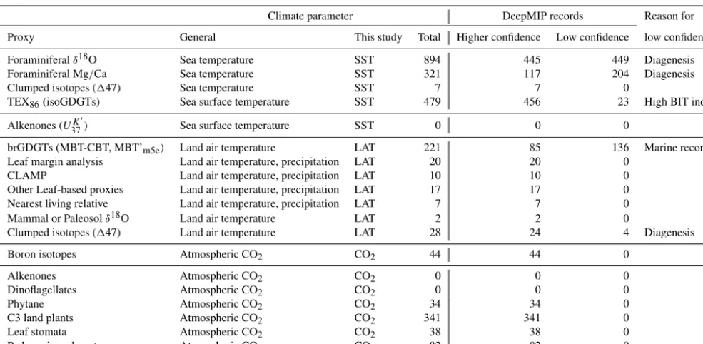
each proxy, we outline (1) the underlying theoretical back-ground, (2) strengths, (3) weaknesses and (4) recommenda-tions on methodologies. We focus on SST and have compiled data from published studies of planktic foraminiferalδ18O (Supplement Data File 3) and Mg/Ca ratios (Supplement Data File 4), clumped isotopes from benthic foraminifera and molluscs (Supplement Data File 5) and TEX86 (Supplement
Data File 6). These data comprise 1701 samples from 40 drill holes or onshore sections.
4.1 Oxygen isotopes
or sub-thermocline depths, or as benthos on or just below the sea floor. Temperature is calculated by an empirical calibration to quantify the fractionation between theδ18O of ancient seawater and biogenic calcite (Bemis et al., 1998). 4.1.2 Strengths of oxygen isotopes
Foraminiferal oxygen isotopes have been the primary proxy for reconstructing ocean temperatures spanning the past ∼ 120 million years, largely due to the low analytical cost, small sample size requirements and relative ease of measure-ment. Analytical uncertainty onδ18O measurements is typ-ically small, ±0.1‰ (equivalent to <1◦C). Moreover, the theoretical basis for temperature-dependent fractionation is firmly tied to field- and laboratory-based relationships be-tween foraminifer test δ18O values and temperature (e.g., Kim and O’Neil, 1997; Bemis et al., 1998; Lynch-Stieglitz et al., 1999). The range of planktic foraminiferal depth habitats also allows for the reconstruction of water column profiles and thermocline structure (e.g., Birch et al., 2013; John et al., 2013), which can be compared to modeled upper ocean structure (e.g., Lunt et al., 2017). The relatively short life span of planktic foraminifera, 2 weeks to 1 month for most modern species, can also provide constraints on paleoseason-ality (Pearson, 2012). Further, based on the assumption that deep-water formation is largely focussed at high (subpolar) latitudes throughout the Cenozoic (Cramer et al., 2011), ben-thic foraminiferal δ18O values can (arguably) be used as a SST proxy in these areas.
4.1.3 Weaknesses of oxygen isotopes
The dissolution and subsequent replacement of pri-mary biogenic calcite by inorganic calcite (recrystalliza-tion/diagenesis) in pelagic, carbonate-rich sediments during early diagenesis is known to shift planktic foraminiferal cal-cite to higher values (Schrag et al., 1995), with the effect that most low- and mid-latitude δ18O-derived Paleogene SSTs from deep-ocean carbonate-rich successions may be system-atic underestimates (Pearson et al., 2001, 2007; Tripati et al., 2003; Sexton et al., 2006; Pearson and Burgess, 2008; Koz-don et al., 2011; Edgar et al., 2015). The effect of seafloor recrystallization and diagenesis on SST estimates will be pro-portionally less significant in areas where cooler surface wa-ters are closer to deep ocean temperatures, which may be the case in some Paleogene high-latitude or upwelling regions, and is considered to be insignificant for benthic foraminifera because temperatures during early diagenesis are very close to growth temperatures (Schrag, 1999; Edgar et al., 2013; Voigt et al., 2016). During diagenesis, foraminifer tests may also become overgrown and/or infilled with calcite precip-itated from sediment pore waters. Where marine sediments are exposed on land, those secondary precipitates can in-corporate oxygen from isotopically light meteoric waters and hence yield artificially warm apparent temperatures. For
these reasons, temperature estimates from foraminiferalδ18O are only considered to be reliable where a good state of preservation has been confirmed by scanning electron micro-scope (SEM) examination and illustration. Well-preserved (non-recrystallized or glassy) late Paleocene to early Eocene foraminifera have been reported from low-permeability clay-rich facies in shallow marine or hemipelagic settings from Tanzania (Pearson et al., 2004; 2009; Sexton et al., 2006), the New Jersey margin and California (Zachos et al., 2006; John et al., 2008; Makarova et al., 2017), New Zealand (Hol-lis et al., 2012), and Nigeria (Frieling et al., 2017).
One key assumption forδ18O-based temperatures is that foraminifera precipitate their tests in isotopic equilibrium with seawater. However, foraminiferal physiology (e.g., respiration, metabolism, biomineralization, photosymbiosis) and ecology (e.g., depth migration during life cycle, season-ality), often termed “vital effects”, commonly lead to isotopic offsets that can bias temperature reconstructions (e.g., Urey et al., 1951; Birch et al., 2013). The biology and ecology of foraminifera may also vary in either time or space. For in-stance, the depth habitat of a species may change in response to rapid environmental change, or due to evolution within a lineage. Foraminifera that host algal photosymbionts may also be subject to bleaching events, which can substantially alter the test micro-environment within which calcification, and the associated isotopic fractionation, occurs (Wade et al., 2008; Edgar et al., 2013; Luciani et al., 2016; Si and Aubry, 2018). In some sites there is evidence that plank-tonic foraminifera and other eukaryotes disappeared from the record during peak PETM warming, possibly because envi-ronmental conditions became too extreme (Aze et al., 2014; Frieling et al., 2018), in which case peak conditions would go unrecorded by this proxy. Enhanced dissolution in the PETM would have the same effect.
Calculating ancient SST from foraminiferalδ18O requires an estimation of the oxygen isotopic composition of sea-water (δ18Osw) at the time of precipitation. This is not
straightforward becauseδ18Osw varies spatially in the
sur-face ocean, largely following patterns of salinity (Zachos et al., 1994; Rohling, 2013), and temporally due to changes in the cryosphere (Broecker, 1989; Cramer et al., 2009). Large and spatially variable changes in the intensity of the hydro-logical cycle are inferred across the PETM (Bowen et al., 2004; Zachos et al., 2006; Pagani et al., 2006; Carmichael et al., 2017); hence it is unlikely thatδ18Oswat any single
loca-tion remained constant through the Paleocene–Eocene inter-val. Continental margin settings, where foraminifera are typi-cally well preserved, may be particularly sensitive to changes inδ18Oswrelated to the hydrological cycle.
different from today (Zeebe, 2001). Studies suggest that early Paleogene surface ocean pH was as much as ∼0.5 units lower than today (Penman et al., 2014; Anagnostou et al., 2016; Gutjahr et al., 2017), which implies that background δ18O-based SST estimates for this time interval could be ∼3◦C too low, or even more so for the PETM when pH may have declined by a further∼0.3 units (Uchikawa and Zeebe, 2010; Aze et al., 2014).
4.1.4 Recommended methodologies for oxygen isotopes Here we outline our recommendations for generating δ18O data from fossil foraminifera, and for converting δ18O val-ues into temperature estimates. We have compiled available planktic foraminiferal δ18O data from 10 DSDP, ODP and IODP sites and 9 onshore sections (Supplement Data File 3). Using the methods outlined below, we have calculated SSTs and compiled a summary of proxy-specific SST esti-mates for each time slice (LP, PETM, EECO). SST estiesti-mates are based on species that are inferred to have inhabited near-surface waters or the mixed layer. Data for deeper-dwelling (thermocline) planktic species are also included in Supple-ment Data File 3. For compilations of benthic foraminiferal δ18O, see Zachos et al. (2008), Cramer et al. (2009, 2011) and Westerhold et al. (2017, 2018), although these data are not considered here.
Depth ecologies of all Paleogene species, as inferred mainly from stable isotope evidence, have been compiled by Aze et al. (2011). The principal groups used for sea sur-face temperature reconstruction are open-ocean mixed-layer species with or without algal symbionts and high-latitude species (ecogroups 1, 2 and 5 of Aze et al., 2011). The main mixed-layer genera for the DeepMIP time slices are Moro-zovellaandAcarininabut other relevant groups areIgorina, Planorotalites and Pseudohastigerina. Different species of Morozovella and Acarinina may exhibit consistent offsets indicating a degree of depth stratification within the mixed layer and upper thermocline, possibly related to sinking at the time of reproduction. Hence SST reconstructions from different “mixed layer” species may vary by up to several de-grees Celsius. Because of this, combining various species of the same genus in analyses (e.g., measuringAcarininaspp.) is likely to produce underestimates of SST. In this compila-tion, we derive average SST estimates from “mixed layer” species for each site in a given time slice. This is to promote consistency and aid intersite comparisons but is considered to be a conservative approach to estimating SSTs. For fu-ture work we recommend more detailed investigation of the various important species and identification of those species which most faithfully record the warmest upper ocean mixed layer conditions.
To expand on the δ18O database, we propose a three-pronged approach. First, analysis of new and classic carbonate-rich sites containing recrystallized foraminiferal tests should involve the novel technique that uses a secondary
ion mass spectrometer (SIMS). Pioneering SIMS studies by Kozdon et al. (2011, 2013) suggest that areas furthest from the test exterior are less susceptible to diagenetic overprint-ing. These areas yield SSTs up to∼8◦C warmer than con-ventional analyses from the same sample and are in better agreement with δ18O-based SSTs from glassy tests (Koz-don et al., 2011). On a cautionary note, a recent study by Wycech et al. (2018) has reported an offset between SIMS and traditional isotope-ratio mass spectrometer (IRMS) anal-yses for modern foraminifera, with SIMSδ18O values being ∼0.9‰ lower. Further study is needed to determine if this offset also affects fossil foraminifera. The SIMS technique provides hope for recovering reliable SSTs from recrystal-lized foraminiferal tests but it is time intensive and is not a practical approach for the analysis of all samples. Thus, our second recommendation is that whole specimen analy-ses are undertaken together with the SIMS analysis, in or-der to constrain the magnitude of diagenetic bias on IRMS δ18O values. For lithologically uniform sediments, quantita-tive estimates of this diagenetic bias in a few widely spaced samples could provide calibration points for higher resolu-tion data generated by convenresolu-tional whole shell methods. Whole specimen isotopic analyses should be species-specific and use a prescribed size fraction (e.g., 250–300 µm or 300– 355 µm) to minimize variations in vital effects (Birch et al., 2013). Our third recommendation is that new sites that con-tain glassy foraminifera are sought out to provide the mate-rial for whole specimen analysis, as well as SIMS analysis of selected samples to further validate the two methods. All samples included within the database are categorized as ei-ther glassy or recrystallized, using the criteria of Sexton et al. (2006) and Pearson and Burgess (2008), as a guide to re-constructed SST reliability.
Empirically derived δ18O–temperature calibrations can differ by several degrees Celsius, , although offsets decrease with increasing temperature (Bemis et al., 1998; Pearson, 2012). Use of multiple equations may capture a range of plausible temperature values but our preference is the cal-ibration of Kim and O’Neil (1997) for inorganic calcite, which is appropriate for the Paleogene because it is based on inorganic calcite precipitated from water temperatures be-tween 10 and 40◦C. Both epibenthic and asymbiotic plank-tic foraminifera yield values close to the resulting regression (Bemis et al., 1998; Costa et al., 2006). Field or laboratory studies only include calcite precipitated up to 30◦C (e.g., Bemis et al., 1998; Lynch-Stieglitz et al., 1999), yet Pale-ogene SSTs likely fall close to or above the upper limit of these studies. The recommended calibration, as modified by Bemis et al. (1998), derives temperature from Eq. (1): T =16.1−4.64(δ18OC−δ18Osw)
+0.09(δ18OC−δ18Osw)2, (1)
where T is the water temperature in ◦C and δ18OC and
sea-water (‰ VSMOW), respectively. This equation may over-estimate SST for symbiont-hosting planktic foraminifera by ∼1.5◦C based on the consistent 0.3 ‰ offset observed be-tweenOrbulina universagrown under high-light compared to low-light conditions (Spero and Williams, 1988; Pear-son, 2012). This offset is likely caused by algal photosym-bionts modifying the pH in the calcifying microenvironment (Zeebe et al., 1999).Orbulina universais inferred to share a similar ecology to the dominant Eocene generaMorozovella andAcarininatypically analyzed for Paleogene SSTs (e.g., Shackleton et al., 1985; D’Hondt et al., 1994) and is cur-rently the best modern analogue for which calibration data are available. However, we do not recommend applying a symbiont correction to these genera because of uncertainties in photosymbiont activity levels in Paleogene conditions.
It is assumed that these δ18O calibrations are insensitive to evolving seawater chemistry, unlike some trace element proxies (e.g., Evans and Müller, 2012). These calibrations do, however, require an appropriate estimate ofδ18Oswat the
time of test formation. Changes in global meanδ18Osw are
largely driven by continental ice volume and isotopic com-position. Various estimates have been proposed for the ad-justment of the global ocean value for ice-free conditions of the early Paleogene: Shackleton and Kennett’s (1975) initial estimate of −1.00 ‰ can be compared with the more re-cent estimates of −1.11 ‰ of L’Homme et al. (2005) and −0.89 ‰ of Cramer et al. (2011). Differences arise from un-certainty surrounding the mean δ18O value of the modern ice caps (see Pearson, 2012 for discussion). Pending reso-lution of these discrepancies we here use the value−1.00 ‰ for early Paleogeneδ18Oswunder ice-free conditions, which
is the mean of the L’Homme et al. (2005) and Cramer et al. (2011) estimates and identical to the estimate of Shackle-ton and Kennett (1975) upon which many historical temper-ature estimates have relied. A correction for the local effects of salinity and hydrology onδ18Oswshould also be
incorpo-rated into SST estimates where possible. Zachos et al. (1994) developed a correction using present-dayδ18Oswlatitudinal
gradients, which is widely used despite acknowledged short-comings. The correction is applied globally but is only based on Southern Hemisphere data and does not incorporate local freshwater runoff effects on continental margins or the influ-ence of boundary currents. It also ignores expected changes in the relationship between latitude andδ18Oswthrough time.
Isotope-enabled climate models have been used to generate predictions of early Paleogene surface oceanδ18Osw
distri-butions, following an assumption of mean average δ18Osw
conditions (e.g., Tindall et al., 2010; Roberts et al., 2011), but theδ18Oswfields generated are dependent on the surface
climatology of the model concerned (Hollis et al., 2012). The use of model-derivedδ18Oswto generate proxy estimates of
SST also introduces a problematic model-dependency within the proxy dataset. Here, we chose to update the approach of Zachos et al. (1994) using the more highly resolved global gridded (1◦×1◦) dataset of modern δ18Osw produced by
LeGrande and Schmidt (2006). We calculated δ18Osw for
each site by relating the site’s paleolocation to 10◦ latitudi-nal bins in the modern dataset (see Supplement Data File 3). Median values and 95 % confidence intervals were calculated using paleolocations derived from both paleomagnetic and mantle-based reference frames (see Sect. 7.2). We encourage future studies to improve the empirical fit to the modern spa-tial variability inδ18Oswbut also recognize that the modern
system only provides a first-order estimate of spatialδ18Osw
patterns in deep time. With improved data coverage, paired δ18O–Mg/Ca andδ18O–147 analyses hold promise for di-rect reconstructions of ancientδ18Oswvariability.
We do not recommend applying a pH correction toδ18O data because of significant uncertainty in the magnitude of the effect below pH 8 (Uchikawa and Zeebe, 2010), which is inferred to be the upper limit for most of our Paleogene records (Anagnostou et al., 2016; Penman et al., 2014; Gut-jahr et al., 2017). Further, the pH–δ18OCsensitivity of
asym-biotic planktic and benthic foraminifera is not well known (e.g., Anagnostou et al., 2016; McCorkle et al., 2008; Mack-ensen, 2008).
4.2 Mg/Ca ratios
4.2.1 Theoretical background of Mg/Ca ratios
The sensitivity of foraminiferal Mg/Ca ratios to temper-ature has a basis in thermodynamics (Lea et al., 1999) through the exponential temperature dependence of any re-action for which there is an associated change in enthalpy. However, most species do not conform to theoretical calcula-tions (Rosenthal et al., 1997), being characterized by a tem-perature sensitivity of Mg incorporation around 2–3 times greater than that for inorganic calcite. The reasons for this remain elusive (e.g., Bentov and Erez, 2006), necessitating empirical calibration of foraminiferal Mg/Ca to temperature (e.g., Anand et al., 2003).
4.2.2 Strengths of Mg/Ca
As withδ18O paleothermometry, Mg/Ca paleothermometry can be applied to both benthic and planktic foraminifera and be used to constrain the past thermal structure of the water column (Tripati and Elderfield, 2005). The long residence time of Ca and Mg in the ocean means that the Mg/Ca of seawater (Mg/Casw) can be treated as constant over short
timescales (<106years), which removes one source of un-certainty in calculating relative changes in temperature (e.g., Zachos et al., 2003; Tripati and Elderfield, 2004). A ma-jor advantage of Mg/Ca is its use in paired measurements withδ18O on the same substrate, which allows for the de-convolution ofδ18Oswand temperature effects on measured
high-resolution time series are readily achievable. Techno-logical developments in laser-ablation inductively coupled plasma mass spectrometry (ICPMS) and other spatially re-solved methodologies, such as electron probe microanalysis (EPMA) and SIMS, allow for Mg/Ca measurements on or within a single individual test, providing new information on foraminiferal ecology and short-term environmental variabil-ity (e.g., Eggins et al., 2004; Evans et al., 2013; Spero et al., 2015). Planktic foraminiferal Mg/Ca may also be more ro-bust to shallow burial diagenetic recrystallization thanδ18O, based on values measured in the same material (Sexton et al., 2006).
4.2.3 Weaknesses of Mg/Ca
A long-standing challenge for the deep-time application of the Mg/Ca temperature proxy is that the seawater Mg/Ca ratio (Mg/Casw) influences shell Mg/Ca, but there is still
de-bate over how Mg/Caswhas varied through time (Horita et
al., 2002; Coggon et al., 2010; Broecker and Yu, 2011; Evans and Müller, 2012). Nonthermal influences on foraminiferal Mg/Ca ratios can also be difficult to account for, includ-ing pH, bottom water carbonate saturation state and sample contamination (Barker et al., 2003; Regenberg et al., 2014; Evans et al., 2016b). Determining the reliability of Mg/Ca paleotemperatures requires an understanding of these chal-lenges, and the use of independent paleoenvironmental prox-ies where available, such as boron isotopes to constrain car-bonate system parameters (Anagnostou et al., 2016).
Impact of foraminiferal preservation on the Mg / Ca pale-othermometer. Many foraminifer tests from deep ocean sed-iments are affected by diagenetic alteration (Pearson et al., 2001; Edgar et al., 2015), with the type and extent of al-teration controlled by original test morphology, taphonomic processes, the characteristics of the host sediment and burial history. For example, planktic foraminifera tests can un-dergo immediate post-mortem or post-gametogenic dissolu-tion as they sink into deeper, less carbonate saturated wa-ters (Brown and Elderfield, 1996). In general, MgCO3 is more soluble than CaCO3such that dissolution tends to
de-crease foraminiferal Mg/Ca. This may result in artificially low Mg/Ca-based temperature estimates if unaccounted for (e.g., Rosenthal and Lohmann, 2002; Regenberg et al., 2014; Fehrenbacher and Martin, 2014), although not in all cases (e.g., Sadekov et al., 2010; Fehrenbacher and Martin, 2014). The effects of dissolution can be minimized by selecting sites with relatively shallow paleodepths, above the calcite lyso-cline (e.g.,<2000 m). Foraminiferal shells can also be sub-ject to diagenetic overgrowths of various mineral phases, in-cluding oxy-hydroxides and authigenic carbonates, depend-ing on seafloor and sub-seafloor conditions (e.g., Boyle, 1983). Recent work suggests that some textural recrystalliza-tion of planktic foraminiferal tests may occur in semiclosed chemical conditions, potentially allowing original
geochem-ical signals to be retrieved using microsampling techniques (e.g., Kozdon et al., 2011, 2013, see Sect. 5.2.5).
Challenges for benthic foraminiferal Mg / Ca paleother-mometry. The temperature sensitivity of Mg incorporation into benthic foraminiferal calcite varies between species, ne-cessitating genus- or species-specific temperature calibra-tions (Lear et al., 2002). Fortunately, some extant species are common throughout the Cenozoic (e.g.,Oridorsalis um-bonatus – Lear et al., 2000) and offer a means to develop calibrations for coeval extinct species. There is also no con-sensus as to whether relationships between benthic Mg/Ca and temperature are best described by linear or exponential fits (Cramer et al., 2011; Evans and Müller, 2012; Lear et al., 2015); we recommend that calibrations are applied with caution where Mg/Ca ratios are outside the range for which temperatures have been empirically determined.
Present-day benthic foraminifera appear to increase their discrimination against magnesium when calcifying in waters with very low carbonate ion saturation state (1CO23−); a rela-tionship that has been empirically quantified for some species (Elderfield et al., 2006; Rosenthal et al., 2006). Measure-ments of benthic foraminiferal B/Ca in tandem with Mg/Ca can be used to identify temporal variations in1CO23− (Yu and Elderfield, 2007) and may provide a means of correct-ing for this secondary effect, although it can be difficult to identify the threshold for a1CO23− influence within down-core records (e.g., Lear et al., 2010). Mg/Li ratios may have a more consistent empirical relationship with temperature than Mg/Ca (Bryan and Marchitto, 2008). However, lim-ited understanding of how the Mg/Li seawater ratio has var-ied over geological time means that this proxy can only be used as a guide to relative temperature change in deep time studies (Lear et al., 2010). The calcification of endoben-thic foraminifera species within buffered porewaters may make them relatively insensitive to variations in bottom water 1CO23−(Zeebe, 2007; Elderfield et al., 2010). However, the saturation state of porewaters is dependent on many factors and likely also varies through time (Weldeab et al., 2016). We recommend that tandem trace metal ratios that are sen-sitive to carbonate saturation state (e.g., B/Ca, Li/Ca) are examined to assess downcore1CO23−variations, even in in-faunal records (e.g., Lear et al., 2010, 2015; Mawbey and Lear, 2013).
Evidence from multiple proxies indicates that early Paleo-gene Mg/Caswwas significantly lower than the modern value
(Horita et al., 2002; Coggon et al., 2010; Lear et al., 2015; Evans et al., 2018a). Correcting benthic Mg/Ca data for sec-ular changes in seawater chemistry is complicated by the fact that the benthic foraminiferal magnesium partition co-efficient (DMg=Mg/CaCALCITE/Mg/Casw)decreases with
increasing Mg/Casw according to a power function (Ries,
2004; Hasiuk and Lohmann, 2010; Evans and Müller, 2012; Lear et al., 2015). Moreover, the sensitivity of shell Mg/Ca to changes in Mg/Casw, specifically the curvature of the power
genus-specific. Lear et al. (2015) and Evans et al. (2016b) argued for a low sensitivity of shell Mg/Ca to Mg/Casw for Ori-dorsalis and the endobenthic genusUvigerina. In contrast, a higher sensitivity is thought to characterize the epibenthic genus Cibicidoides/Cibicides (Evans et al., 2016b), which is also widely used in paleoclimate studies. Evaluating this aspect of benthic foraminiferal geochemistry is challenging and has yet to be assessed in other widely utilized species. As such, best practice would be to report to what extent Mg/Ca temperatures would change when considering the uncertainty in the slopes of these seawater–shell Mg/Ca relationships.
Challenges for planktic foraminifera Mg / Ca. The rela-tionship between planktic Mg/Ca ratios and temperature is species- or group-specific (e.g., Regenberg et al., 2009), such that species-specific calibrations should be used whenever possible. Nonetheless, many planktic foraminifera conform to a broader Mg/Ca–temperature relationship (Elderfield and Ganssen, 2000; Anand et al., 2003), which is one method by which modern calibrations can be applied to extinct taxa. As for benthic foraminifera, when working with pre-Pleistocene samples the control exerted by changes in seawater ele-mental chemistry over geological time must also be con-sidered. Culture experiments in modified seawater demon-strate not only that Mg/Caswimpacts planktic foraminifera
shell chemistry (Delaney et al., 1985), but also that the slope of the Mg/Ca–temperature relationship may be sensitive to Mg/Casw (Evans et al., 2016b). In addition, several other
nonthermal controls on Mg/Ca should be considered when interpreting data from planktic foraminifera. Culture and core-top studies demonstrate a relatively minor salinity ef-fect (Kısakürek et al., 2008; Hönisch et al., 2013) in which, for example, a 2 PSU salinity increase results in a tempera-ture overestimate of∼1◦C. In contrast, the carbonate sys-tem has been shown to have a large influence on Mg/Ca in several species (Lea et al., 1999; Russell et al., 2004; Evans et al., 2016a). Lower pH and/or [CO23−] results in higher shell Mg/Ca; for example, a 0.1 unit pH decrease results in a temperature overestimate of ∼1◦C. The effect of the carbonate system on planktic Mg/Ca has been identified in sediment-trap as well as culture studies (Evans et al., 2016a; Gray et al., 2018), with Gray et al. (2018) demonstrating that the widely used Mg/Ca–temperature sensitivity of∼9 % per degree Celsius inGlobigerinoides ruberis an artifact of the covariance of temperature and pH, through the temperature effect on the dissociation constant of water. Specifically, the pH of seawater decreases with increasing temperature, result-ing in an increase in the incorporation of Mg into planktic foraminiferal calcite due to both processes (see Evans et al., 2018b). The secondary pH effect accounts for around one-third of the observed increase in Mg/Ca ratios at higher tem-peratures, leaving a primary Mg/Ca “temperature only” sen-sitivity of 6 % per degree Celsius (Gray et al., 2018), which is significantly lower than that widely utilized. Whilst these factors may be accurately accounted for in the recent geolog-ical past (Gray and Evans, 2019), it is challenging to account
for them in deep time because high-resolution pH records are scarce (see below for detailed recommendations).
4.2.4 Recommended methodologies for Mg/Ca
Here we outline our recommendations for generating Mg/Ca data from fossil foraminifera and for converting these data into temperature estimates. We have compiled available planktic Mg/Ca data from five DSDP and ODP sites and six onshore sections and, using the methods outlined below, cal-culated SSTs and associated uncertainties for the late Pale-ocene and early EPale-ocene (Supplement Data File 4). SST es-timates are based on species that are inferred to have inhab-ited near-surface waters or the mixed layer. Data for deeper-dwelling (thermocline) planktic species are also included in Supplement Data File 4 but are not discussed here. For com-pilations of benthic foraminiferal Mg/Ca ratios, see Cramer et al., 2011).
Sample preparation. Foraminifera need to be thoroughly cleaned prior to analysis. Clay and organic contaminants are removed using a short oxidative procedure, whereas re-moval of metal oxide contaminants requires a longer proce-dure including a reductive step (Boyle and Keigwin, 1985). These two procedures result in offsets in Mg/Ca values, which must be corrected when making comparisons to other records (e.g., Barker et al., 2003; Yu et al., 2007). Clean-ing efficacy is assessed usClean-ing Al/Ca, Mn/Ca and Fe/Ca ra-tios (e.g., Boyle, 1983; Barker et al., 2003). In some cases, a simple threshold value may be used to screen samples, e.g., Al/Ca>80 µmol mol−1 (Mawbey and Lear, 2013). In many cases, the threshold depends on contaminant composi-tion such that Mn/Mg or Fe/Mg ratios may be a more use-ful indicator (Barker et al., 2003). Cleaned foraminifera are commonly dissolved in acid and analyzed by ICPMS, tak-ing into account the dependence of measured Mg/Ca on an-alyte concentration (the matrix effect – Lear et al., 2002), al-though other techniques may also be employed (see below). Prior to crushing, several representative specimens should be selected for SEM analysis to record the extent of textu-ral recrystallization on broken chamber walls. Sr/Ca values routinely collected alongside Mg/Ca data can provide one means of monitoring the impact of recrystallization on test geochemistry. Inorganic calcite tends to have lower Sr/Ca and higher Mg/Ca than foraminiferal calcite (Baker et al., 1982), which leads to inverse relationships in diagenetically altered downcore records.
Recommended steps. The following are recommended steps in converting planktic Mg / Ca ratios to temperatures:
with Mg/Ca data to assess the potential impact of dis-solution (e.g., Rosenthal and Lohmann, 2002). Alter-natively, chemically resistant domains within individual tests can be selected for analysis (see above).
ii. A salinity correction should be applied if there is in-dependent evidence that the sample site experienced substantial deviations from normal salinity, such as the large changes in the hydrological cycle inferred for the PETM (Zachos et al., 2003). Normalizing culture data of three modern species (compiled in Hönisch et al., 2013; Allen et al., 2016) to the Mg/Ca observed at a salinity of 35 psu for each species results in the follow-ing multi-species salinity sensitivity:
Mg/CaCORRECTED=(1−(salinity−35)×0.042±0.008)
×Mg/CaMEASURED
(2) (see the Supplement for further details). This sensitivity of 4.2±0.8 % per PSU is in good agreement with global sediment trap and plankton tow data forG. ruber(Gray et al., 2018).
iii. A correction for past changes in the carbonate system should be applied. This is complicated, however, be-cause pH and [CO23−] are not only driven by long-term changes in the carbon cycle but also by factors such as the temperature effect on the dissociation constant of water (KW). Therefore, whilst the results of Gray et
al. (2018) indicate that the Mg/Ca–temperature sensi-tivity in the modern ocean is 6 % per degree Celsius when the effects of pH and temperature are fully de-convolved, this can only be applied if the control of temperature onKW(and therefore pH) is accounted for
(ideally throughδ11B-derived pH reconstructions using the same material). For instance, if the pH reconstruc-tion available for a given interval was determined at a different site, a temperature sensitivity of 6 % per de-gree Celsius should be applied only if the difference in temperature between sites can be estimated, so that the temperature-driven intersite pH gradient can be ac-counted for (pH differences between sites may also ex-ist for other reasons). In practice, this requires that the equations for pH and temperature be solved iteratively, given that Mg/Ca is sensitive to both factors. We recom-mend differing approaches for Mg/Ca data treatment depending on whether aδ11B pH record is available for the same site (see step v below).
Where δ11B-based pH reconstructions are available, Mg/Ca ratios should be corrected for pH. However, this correction should be considered with caution until the controlling carbonate system parameter on foraminifera Mg/Ca is identified, particularly given that pH and [CO23−] may be decoupled over geological time (Tyrrell
and Zeebe, 2004). If no pH reconstruction is available for the site of interest, then the temporally and spatially closest data should be used and uncertainties in apply-ing this considered. Based on a linear fit through culture data from three modern species (Evans et al., 2016a), the correction is as follows:
Mg/CaCORRECTED=(1−(8.05−pH)×0.70±0.18)
×Mg/CaMEASURED.
(3) Note that Mg/Ca may relate nonlinearly to pH out-side the range 7.7–8.4, and more complex relationships have been suggested (Russell et al., 2004; Evans et al., 2016a). This sensitivity of−7.0±1.8 % per 0.1 pH unit is in agreement with the−8.3±7.7 % derived from a global sediment-trap and plankton towG. ruberdataset (Gray et al., 2018), although we recommend applying the culture-derived expression in deep time because it is calibrated over a much wider pH range.
iv. A correction for Mg/Casw is usually applied to the
pre-exponential component (B) of the relevant Mg/Ca– temperature calibration of the form Mg/Ca = BexpAT (Hasiuk and Lohmann, 2010; Evans and Müller, 2012): BCORRECTED=(Mg/CaswH/5.2H)×BMODERN, (4)
whereBMODERN is the pre-exponential coefficient
de-rived from modern calibrations,H is the nonlinearity of the relationship between shell and Mg/Casw, which
may be estimated from culture experiments under vari-able seawater chemistry (Evans et al., 2016b; Delaney et al., 1985), Mg/Casw is that of the time interval of
interest, and 5.2 is the modern seawater Mg/Ca ratio in moles per mole (mol mol−1). However, the obser-vation that the slope of this relationship is sensitive to Mg/Caswin culture experiments means that equations
describing the change in both constants (AandB) have been reported for modern taxa (Evans et al., 2016b), with the implication that the use of modern calibrations may underestimate relative temperature changes during the early Paleogene. For estimates of early Paleogene Mg/Caswwe recommend the use of a relatively
high-precision, million-year (average) resolution Mg/Casw
reconstruction from the coupled analysis of Mg/Ca and clumped isotopes in foraminifera (Evans et al., 2018a). v. Mg/Ca is converted to temperature using an exponential
calibration equation:
T =ln(Mg/CaCORRECTED/BCORRECTED)/A, (5)
whereAandBCORRECTEDare derived from species or
based on similarities to extant species in terms of shell chemistry or, for example, position within the water col-umn and the presence or absence of symbionts. Best practice would be to report the sensitivity of a recon-struction to the choice of calibration equation. Impor-tantly, the sensitivity factor Ashould be modified pending on how the carbonate system correction de-scribed above is performed. If pH is explicitly ac-counted for at the site of interest throughδ11B then the 6 % per degree Celsius sensitivity of Gray et al. (2018) should be applied. However, if the best available pH re-construction is from a different site or time interval or derived from a model which represents the global mean (e.g., Tyrrell and Zeebe, 2004), then we recommend applying the apparent sensitivity derived from culture (Kısakürek et al., 2008; Evans et al., 2016a) as this in-directly accounts for the effect of temperature onKW.
These recommendations have been applied to the Mg/Ca analyses included in the DeepMIP database (Supplement Data File 4). We have compiled Mg/Ca data for planktic foraminifera from five DSDP or ODP sites and six onshore sections. SST was derived from Mg/Ca ratios as follows: 1000 random draws were performed of salinity (33–37 psu), seawater Mg/Ca (within the 95 % CI given by Evans et al., 2018b), pH (±0.2 units) and the Mg/Ca–pH sensitivity (any-where between 0 %–8.8 % per 0.1 unit, i.e., any(any-where be-tween not sensitive at all to the upper confidence interval on the modern culture calibrations) for each data point. Calibra-tion uncertainty was assessed by randomly choosing either the laboratory calibrations of Evans et al. (2016b), which define a Mg/Casw-dependent Mg/Ca–T sensitivity, or the
modern calibration with an “H-factor” applied to the pre-exponential constant (Evans and Müller, 2012), which main-tains the modern Mg/Ca–T sensitivity in deep time. The un-certainties on each data point are then the 97.5 and 2.5 per-centiles of these 1000 sets of assumptions. The “best esti-mate” SSTs are the 50 percentiles of the subset of these 1000 draws that use the calibrations of Evans et al. (2016b), which is preferred because the available evidence suggests that the Mg/Ca–T sensitivity varies as a function of Mg/Casw. Note
that the data are subject to revision following replication of that study, and that using the 50th percentile of all es-timates including both calibrations would result in overall cooler SST. Analytical uncertainty is not considered signifi-cant given the magnitude of these uncertainties.
Intra-test Mg / Ca analysis by LA-ICPMS and EPMA. In contrast to solution inductively-coupled-plasma mass spec-trometry, which enables high throughput of pooled, dissolved foraminifera, highly spatially resolved techniques such as laser-ablation ICPMS (LA-ICPMS) facilitate targeted in situ analysis of carbonates (Eggins et al., 2003) and allow intra-specimen preservation to be assessed (e.g., Creech et al., 2010; Evans et al., 2015). Small samples such as foraminifera may be analyzed without embedding or sectioning, and
high-sample throughput means that the technique is relatively in-expensive. Laser spot sizes are typically 20–80 µm in di-ameter, with 5 µm possible (Lazartigues et al., 2014), en-abling repeat measurements of individual chambers or sea-sonality reconstruction in long-lived organisms with incre-mental growth layers (Bougeois et al., 2014; Evans et al., 2013). Because each laser pulse removes less than 100 nm of material on carbonates (Griffiths et al., 2013), depth-profiling through the sample has an effective resolution of <0.5 µm when using a fast wash-out ablation cell (Müller et al., 2009). Therefore, element profiles through foraminifera chamber walls not only facilitate the characterization of intra-specimen preservation, which can be assessed by the simultaneous collection of Mg/Ca, Sr/Ca, Mn/Ca, Al/Ca and Fe/Ca ratios, among others, but also allow diagenetically affected areas, such as surface overgrowths, to be excluded from the measurement used to calculate the oceanographic variable of interest (e.g., Hollis et al., 2015; Hines et al., 2017). The disadvantage of LA-ICPMS is that overall data acquisition and reduction is typically more time-consuming compared to solution-based techniques and there is relatively large intra-specimen variability.
Electron probe microanalysis (EPMA) is a microanalytical technique based on the detection of element-characteristic X-rays produced by bombarding the sample with an accel-erated and focused electron beam. For quantitative analy-ses, the intensity of the element-specific X-rays is compared against those of the same elements from chemically well-characterized standards. However, the sensitivity of EPMA is limited, and typically only Mg/Ca and Sr/Ca ratios in foraminiferal shells can be quantitatively measured (e.g., Brown and Elderfield, 1996; Anand and Elderfield, 2005). One advantage of this technique is the high spatial reso-lution; typical beam spot sizes for quantitative analyses in foraminiferal shells is∼2 to 10 µm (e.g., Hathorne et al., 2003). In addition, semiquantitative elemental distribution maps can be acquired with submicron resolution for a larger suite of elements (e.g., Pena et al., 2008), allowing for the identification of diagenetic phases.
foraminifera. The average of multiple Mg/Ca measurements by EPMA from an individual shell is typically comparable to solution-phase data that consume the whole shell (e.g., Hathorne et al., 2003). A major advantage of this method is that it is nondestructive.
4.3 Clumped isotopes
4.3.1 Theoretical background of clumped isotopes The carbonate clumped isotope thermometer is based on the temperature-dependent proportion of13C−18O bonds in car-bonate minerals (Ghosh et al., 2006; Eiler, 2007). The proxy has a direct basis in thermodynamics (Schauble et al., 2006; Hill et al., 2014) and has been applied to a wide range of marine and terrestrial samples, from foraminifera to paleosol carbonates (e.g., Tripati et al., 2010; Snell et al., 2013; Dou-glas et al., 2014). The zero-point energy of atomic bonds de-creases with the mass of the atoms involved, favoring bonds between the rare, heavy isotopes. However, this effect de-creases with increasing temperature, leading to the theoreti-cal and observed decrease of “clumping” of heavy isotopes with increasing formation temperature of the mineral (Eiler, 2007). Excess abundance of13C−18O bonds is abbreviated to 147 and refers to the over-abundance of CO2 with the
composition13C−18O−16O relative to a stochastic distribu-tion of all isotopes (Eiler and Schauble, 2004).147 is
mea-sured on an isotope ratio mass spectrometer after acidifica-tion of the carbonate, in a very similar way to classicalδ18O measurements. The only difference is that the abundance of mass 47 is recorded in addition to the traditional masses 44– 46;δ18O andδ13C are obtained as by-products of the mea-surements and are needed to calculate the expected stochas-tic abundance of13C−18O bonds in the respective sample, which is then compared to the observed abundance to calcu-late147.
4.3.2 Strengths of clumped isotopes
There are three key strengths to this carbonate-based pale-othermometer: (1) both theory and empirical studies demon-strate that the isotopic composition of water exerts no mea-surable control on the clumped isotope signature (Ghosh et al., 2006; Schauble et al., 2006); (2) the technique involves the simultaneous measurement of 147 and δ18O, enabling
the independent and direct calculation of ancient δ18Osw;
(3) many, although not all, biogenic carbonates and inorganic precipitates fall on the same calibration line (e.g., Ghosh et al., 2006; Zaarur et al., 2013; Tang et al., 2014; Tripati et al., 2015). Molluscs and brachiopods (Came et al., 2007; Eagle et al., 2013a; Henkes et al., 2013), foraminifera (Tripati et al., 2010; Grauel et al., 2013; Evans et al., 2018a; Peral et al., 2018; Piasecki et al., 2019), paleosols (Passey et al., 2010), land snails (Eagle et al., 2013b), and other forms of carbon-ate (Eiler, 2007; Kele et al., 2015) all appear to be reliable
archives for the measurement of147. Clumped isotope
anal-ysis of speleothems and certain coral species (Ghosh et al., 2006; Tripati et al., 2010, 2015; Saenger et al., 2012; Affek and Zaarur, 2014; Loyd et al., 2016; Spooner et al., 2016) as well as other taxa (Davies and John, 2019) are more uncer-tain and require further study.
4.3.3 Weaknesses of clumped isotopes
Whilst clumped isotope thermometry has been successfully applied to a wide range of sample types, there are several challenges associated with paleoclimate reconstructions. Of these, the most fundamental is the low abundance of doubly substituted (“clumped”) carbonate, which typically makes up only∼46 ppm of the total CO2 produced from a
sam-ple. Precision is therefore ultimately limited by our ability to cleanly measure mass 47 CO2. In practice, this implies
rel-atively large sample masses, typically∼10 mg of material (>500 planktic foraminifera), although recent advances in instrumentation have seen this reduced by a factor of 5–10 in some laboratories (Meckler et al., 2014; Müller et al., 2017). Analytical precision for these sample sizes limits the accu-racy of the technique to±2–3◦C (1 sigma), which can be improved by performing a greater number of replicate mea-surements (e.g., Huntington et al., 2009; Thiagarajan et al., 2011; Tripati et al., 2014), with an obvious trade-off between sample size and precision. The presence of organic carbon, which can contribute to mass 47, may necessitate stringent sample cleaning procedures. In common with many proxies, the potential for seasonal growth of some archives must be considered. This is particularly the case for molluscs. Careful sample selection and geological context are of critical impor-tance when designing studies and interpreting clumped iso-tope data.
As forδ18O and Mg/Ca, the preservation of foraminifera and other carbonates is a key issue that must be addressed. While the impacts of dissolution are not known, recrys-tallization at different temperatures or the addition of sec-ondary diagenetic calcite precipitated after deposition can bias clumped isotope measurements of planktic foraminifera (Shenton et al., 2015; Stolper et al., 2018). However, recent work has shown that glassy foraminifera and some nonglassy planktic and benthic foraminifera appear to yield reliable clumped isotope data for paleoceanographic reconstructions (Leutert et al., 2019). Solid-state reordering within the cal-cite mineral will alter the isotope ordering, although only in samples that have experienced burial temperatures well above 100–150◦C for over ∼10 Ma (Passey and Henkes, 2012; Henkes et al., 2014; Shenton et al., 2015).
Several empirical calibrations of147to temperature have
calibrating biogenic carbonates, whereas calibrations with larger temperature ranges (>90◦C) across different types of carbonates agree well (Bonifacie et al., 2017; Fernandez et al., 2017; Kelson et al., 2017). Material-specific calibrations have also been suggested, for example, for marine molluscs (Eagle et al., 2013b; Henkes et al., 2013). Accurate absolute temperature reconstructions depend on empirical calibrations being developed or checked in each laboratory. Differences between laboratories have been attributed to a range of fac-tors (Dennis et al., 2011; Wacker et al., 2014; Defliese et al., 2015; Daëron et al., 2016; Schauer et al., 2016) but are not yet fully resolved. With the use of rigorous standardization procedures to correct for instrument drift and more consis-tent methodologies overall, it is hoped that calibrations be-tween instruments and labs will converge (e.g., Bernasconi et al., 2018).
4.3.4 Recommended methodologies for clumped isotopes
Here we outline our recommendations for generating clumped isotope data from fossil shells, and for convert-ing these data into temperature. The current dataset for the targeted age range is limited to five early Eocene onshore sections (Supplement Data File 5) and paleosol carbonate data from four continental North American sites (Supple-ment Data File 7A). Using the methods outlined below, we have calculated SSTs and error values and compiled a sum-mary of SST estimates for these EECO sites.
We recommend the use of a calibration that covers a wide temperature range and sufficiently replicated analyses of cal-ibration samples from the carbonate type being analyzed, performed with the same analytical and data processing pro-cedures as those employed for the samples (e.g., in the ab-solute reference frame as defined by Dennis et al., 2011, and done using either gas-standard- or carbonate-standard-based reference frames of Dennis et al., 2011, or the carbonate standard-based reference frame of Bernasconi et al., 2018). Where possible, we recommend that previously published calibrations be converted to these reference frames.
A recent meta-analysis of synthetic carbonate calibrations (Petersen et al., 2019) explores the causes of interlabora-tory offsets and makes recommendations on best practice. Best practice for measuring, correcting and reporting147
in-cludes (1) measurement of a large number of gas and/or car-bonate standards of different compositions; (2) correction for instrumental nonlinearities (Huntington et al., 2009; Dennis et al., 2011), such as those which arise from secondary elec-trons (He et al., 2012; Bernasconi et al., 2013), or use of in-struments with electron suppression; (3) reporting of data on an absolute reference frame (Dennis et al., 2011); and (4) re-porting full methodology, including digestion apparatus, di-gestion temperature, gas cleaning procedure, mass spectrom-eter and corrections used, working gas composition, constant sets used for calculations, acid digestion fractionation factor,
147values and errors, temperature calibration, and estimated
temperatures. Ideally, the provision of gas and/or carbonate standard results together with the sample data facilitates the broad use of data and future recalculations. We recommend the open archiving of raw intensity values and datasets, with their own digital object identifiers, to enable the reanalysis of data over the long term.
Given the required sample amounts and time-intensive measurements, clumped isotope thermometry is most pow-erful where other proxies are limited by unknown confound-ing effects. Rather than providconfound-ing high-resolution recon-structions, clumped isotopes can be used to ground-truth and improve the accuracy of other proxies, including new constraints on seawater compositions (Evans et al., 2018a). Additionally, systems allowing the repeated measurement of small (∼100–500 µg) sample aliquots give the required replication rates for 147, which are averaged across
repli-cates or adjacent samples, and have the potential to provide higher-resolution records of standardδ18O andδ13C analy-ses. As forδ18O and Mg/Ca, samples need to be carefully screened for diagenetic alteration.
4.4 Isoprenoidal GDGTs (TEX86)
4.4.1 Theoretical background of TEX86
The tetraether index of tetraethers consisting of 86 car-bon atoms (TEX86) is an organic paleothermometer based
on the distribution of isoprenoidal glycerol dialkyl glyc-erol tetraethers (isoGDGTs) in marine or lake sediments (Schouten et al., 2002)., Within marine environments, isoGDGTs are inferred to be mainly derived from ma-rine Thaumarchaeota (Schouten et al., 2002; Wuchter et al., 2004). Marine Thaumarchaeota occupy much of the epipelagic and mesopelagic zone, but cell numbers are high-est in the upper few hundreds of meters of the surface ocean (Church et al., 2010), with TEX86 correlating most strongly
with sea surface (SST) or shallow subsurface (sub-T, 50– 200 m) temperatures (Tierney and Tingley, 2015). The under-lying principal of TEX86is that the number of cyclopentane
rings (moieties) in GDGTs increases with growth tempera-ture in order to alter the fluidity and permeability of the cell membrane (Sinninghe Damsté et al., 2012). Laboratory cul-ture and mesocosm experiments confirm this relationship and indicate that TEX86 values continue to increase with
tem-perature above 30◦C (Wuchter et al., 2004; Schouten et al., 2007; Pitcher et al., 2009; Kim et al., 2010), the upper limit of the modern coretop dataset (Kim et al., 2010; Tierney and Tingley, 2015). Although these studies suggest that a lin-ear relationship between TEX86and temperature persists at
least to 40◦C, the form of the relationship has been shown to vary significantly between different strains of Thaumar-chaeota (Elling et al., 2015).
TEX86 has been widely used to reconstruct SST during