Optimal design of a climatological network: beyond practical considerations

(1)

Geosci. Instrum. Method. Data Syst., 2, 199–212, 2013 www.geosci-instrum-method-data-syst.net/2/199/2013/ doi:10.5194/gi-2-199-2013

EGU Journal Logos (RGB)

Advances in

Geosciences

Open Access

Natural Hazards

and Earth System

Sciences

Open Access

Annales

Geophysicae

Open Access

Nonlinear Processes

in Geophysics

Open Access

Atmospheric

Chemistry

and Physics

Open Access

Atmospheric

Chemistry

and Physics

Open Access Discussions

Atmospheric

Measurement

Techniques

Open Access

Atmospheric

Measurement

Techniques

Biogeosciences

Open Access Open Access

Biogeosciences

Discussions

Climate

of the Past

Climate

of the Past

Discussions

Earth System

Dynamics

Earth System

Dynamics

Discussions

Geoscientific

Instrumentation

Methods and

Data Systems

Open Access

_{Geoscientific}

Instrumentation

Methods and

Data Systems

Geoscientific

Model Development

Geoscientific

Model Development

Discussions

Hydrology and

Earth System

Sciences

Open Access

Hydrology and

Earth System

Sciences

Ocean Science

Discussions

Solid Earth

Discussions

The Cryosphere

Discussions

Natural Hazards

and Earth System

Sciences

Open Access

Discussions

Optimal design of a climatological network:

beyond practical considerations

G. S. Mauger1, K. A. Bumbaco2, G. J. Hakim3, and P. W. Mote4

1_{Climate Impacts Group, University of Washington, P.O. Box 355674, Seattle, WA 98195-5672, USA}

2_{Office of the Washington State Climatologist, University of Washington, P.O. Box 355672, Seattle, WA 98195-5672, USA} 3_{Department of Atmospheric Sciences, P.O. Box 351640, University of Washington, Seattle, WA 98195-1640, USA} 4_{College of Earth, Ocean, and Atmospheric Sciences, 104 CEOAS Admin Building, Oregon State University,} Corvallis, OR 97331, USA

Correspondence to: G. S. Mauger ([email protected])

Received: 2 January 2013 – Published in Geosci. Instrum. Method. Data Syst. Discuss.: 3 May 2013 Revised: 1 July 2013 – Accepted: 16 July 2013 – Published: 22 July 2013

Abstract. Station locations in existing environmental

net-works are typically chosen based on practical constraints such as cost and accessibility, while unintentionally over-looking the geographical and statistical properties of the information to be measured. Ideally, such considerations should not take precedence over the intended monitoring goal of the network: the focus of network design should be to adequately sample the quantity to be observed.

Here we describe an optimal network design technique, based on ensemble sensitivity, that objectively locates the most valuable stations for a given field. The method is com-putationally inexpensive and can take practical constraints into account. We describe the method, along with the details of our implementation, and present-example results for the US Pacific Northwest, based on the goal of monitoring re-gional annual-mean climate. The findings indicate that op-timal placement of observing stations can often be highly counterintuitive, thus emphasizing the importance of objec-tive approaches. Although at coarse scales the results are generally consistent, sensitivity tests show important differ-ences, especially at smaller spatial scales. These uncertain-ties could be reduced with improvements in datasets and im-proved estimates of the measurement error. We conclude that the method is best suited for identifying general areas within which observations should be focused, and suggest that the approach could serve as a valuable complement to land sur-veys and expert input in designing new environmental ob-serving networks.

1 Introduction

Environmental observing networks are established for a wide variety of purposes, ranging from short-term weather fore-casting to monitoring ecosystem change. A compromise be-tween scientific and practical considerations (e.g., site ac-cessibility, cost, land ownership) usually governs the place-ment of stations, though practical considerations often have a greater influence on the final station locations. Historically, station site selection has typically been made subjectively, which suggests that the goals for the network are not met optimally or cost effectively. Theories for optimal observing networks have matured to the point where an objective cost-benefit analysis can be considered when creating, augment-ing, or revising an observing network. Objectivity is impor-tant because results show that optimally selected station lo-cations often do not follow from intuition. Here we describe a flexible ensemble-based network-design algorithm that in-corporates measurement error and can account for practi-cal considerations such as accessibility of the site and land ownership.

(2)

is more costly for remote stations, and these locations are of-ten overlooked. For areas with complex terrain such as the western United States, low-lying networks near population centers do not accurately represent the climate in adjacent mountainous areas, especially for precipitation (Dabberdt and Schlatter, 1996). Variations in wind and sun exposure, cold air pooling in mountain valleys, and coastal fog are just a few examples of common weather occurrences that can result in sharp climate distinctions across fairly short dis-tances (e.g., Lundquist and Cayan, 2007; Abatzoglou et al., 2009). As a result, it is possible for closely spaced stations to sample vastly different climates, or conversely, for two dis-tant stations to be highly correlated and hence largely redun-dant. Prior studies have confirmed this (e.g., Fujioka, 1986; Hargrove et al., 2003), showing that uniformly spaced sta-tions do not provide an advantage over those that are opti-mally placed. Fujioka (1986), for example, found that the op-timal station locations were non-intuitive, and had 15 times less normalized error than the gridded locations in represent-ing fire weather variables in southern CA.

Clearly, methods are needed that can help objectively iden-tify compromises between scientific and practical consider-ations when designing and augmenting an observing net-work. By optimally determining the most valuable obser-vation sites, the utility of a network can be maximized and the cost minimized as redundancy and guesswork in station placement is reduced.

2 Methods

2.1 Ensemble sensitivity

The ensemble sensitivity approach to network design is based on the idea of adaptive (or targeted) observations (e.g., Bergot et al., 1999; Morss et al., 2001; Bishop and Toth, 1999). Although the criteria are quite different, the same principles can be applied to the development of a fixed net-work for long-term monitoring. The problem centers on im-proving estimates of a scalar measure of interest, or “met-ric”,J. Applied to network design, the method (e.g., Khare and Anderson, 2006; Ancell and Hakim, 2007; Huntley and Hakim, 2010) works by iteratively finding sites that explain the most variance of a given climate field while accounting for the variance explained by previous “stations” selected (hereafter, the term “station” is used to refer to the opti-mal observing locations identified in the ensemble sensitiv-ity approach). Finding the first station is relatively straight-forward: it consists of identifying the point with the high-est correlation with the metric while also maximizing the ratio of that correlation to the measurement error. Locating the second station is more difficult because the choice must account for the variance already explained by the first sta-tion. As discussed below, this is accomplished by using the Kalman update equation to adjust the sampled values at each

grid point. The process then repeats: a new station is chosen, and the ensemble sample is adjusted to account for the new information that this station provides. With each chosen sta-tion, the variance in the data decreases according to the vari-ance explained by the previous stations. At some point, very little additional variance is gained by identifying new sta-tions, or alternatively, the remaining variance becomes in-distinguishable from the noise. This point is reached when no new information is gained by adding stations beyond the number already identified (in Sect. 2.4 we describe our boot-strap approach to approximating this threshold). Note that the method is general: no specific time step, variables, or spatial configuration is required – this is a key strength of the ap-proach. A brief description of the algorithm follows.

In ensemble sensitivity analysis, different samples of the state of the system (x) are used to develop statistics that relate changes in the state of the system to changes in a particular metric of interest (J). Using a gridded “truth” field as a proxy for observations, an optimally located observation is thus de-fined as the grid point that contributes most to the variance in

J, our metric of interest. We accomplish this by calculating the change in the variance ofJ (1σ_J2) for each grid point, and identifying the grid point for which this change is maxi-mized. By using anomalies in the state of the system (x) and a first-order Taylor expansion ofJ, Ancell and Hakim (2007) show that1σ_J2can be rewritten as follows:

1σ_J2=σ_J,i2 ₋₁−σ_J,i2 (1)

=

_∂_J

∂x

T

KiHiBi−1 _∂_J

∂x

(2)

Ki =Bi−1HTi E

−1

i (3)

Ei =HiBi−1HTi +R2, (4) where i refers to the i-th iteration of the algorithm, Bi−1 is the prior error covariance of x, Ki is the Kalman gain (Hamill, 2006; Kalman, 1960), Eiis the “innovation error co-variance”, andR2is the measurement error, which includes both instrument and “representativeness” error (error associ-ated with sub-grid variability). Hi is a linearized observation operator, which maps the state of the system (x) to an obser-vation of interest. In Eq. (2), the change in the error covari-ance upon selection of thei-th station is estimated using the Kalman gain (Eq. 3) associated with the new observation.

(3)

1σ_J2= cov J, xm,i

2

σ2

xm,i +R

2

m

(5)

xm,i =xm,i−1−β

cov xm,i−1, xstn,i−1 σ2

xstn,i−1 +R

2

m

!

xstn,i−1 (6)

β = 1

1+

r

R2

m

σ2

x_stn_,i₋₁+R2m

, (7)

wherexmrefers to the time series for an arbitrary grid point, xstnrefers to the time series for thei-th selected station, and β is a term that results from the conversion from matrix to square root form (Potter, 1964). These simplified equations arise from the fact that, in serial processing (i.e., the square root implementation), Hi is simply a vector that extracts the mth grid point ofx(i.e., Hi= [0, 0, . . . , 1, . . . , 0]; see Huntley and Hakim, 2010).

Although perhaps less elegant than in their matrix form, these equations help illustrate the logic behind the approach. First, note that Eq. (5) very closely resembles the square of the correlation betweenJ and the time series at each grid point, the only differences being a missing constant (σ_J2) and an added error term (R2) in the denominator. At each step in the calculation, the optimal station is selected by identi-fying the grid point for which1σ_J2is maximized. The error term serves to promote areas where the correlation withJ

is large compared to the measurement uncertainty. Second, note that Eq. (6) essentially uses an ordinary least squares re-gression, scaled byβ, to adjust the sample values at each grid point (xm). The conditional adjustment is thus achieved by removing that portion of the variance inxmthat can be repro-duced using the time series of the selected station (xstn). Fi-nally, note that the parameterβis always between 0.5 and 1, and thus serves to reduce the adjustment toxm, based on the proportion of grid cell variance to measurement uncertainty (R2_).

The approach we have described rests on several key as-sumptions. Specifically, the Kalman update equation is only optimal if the following conditions are met:

1. Linear: the approach involves a linearization about the time-averaged state.

2. Gaussian: the model state variables (and associated noise) are Gaussian in distribution.

These assumptions are discussed in Sect. 2.2 below.

2.2 Data

We apply the approach to the problem of monitoring re-gionally and annually averaged precipitation and temperature over the US Pacific Northwest (hereafter “PNW”), which we define to span the three US states of Idaho, Oregon, and Washington (see Fig. 1). This is based loosely on the re-cent interest in improving climate monitoring across the US,

Ca

sca

d

e

Ra

n

g

e

R

_o

c

k

_y

M

o

u

n

t a

i n

s

Olympic Mtns Canada USA Sn

ake River Plain Seattle

Portland

Boise

W a s h i n g t o n

I d a h o

O r e g o n

Fig. 1. Map of the study region, defined as the region encompassed

by the US states of Idaho, Oregon, and Washington. The map and legend highlight several geographic features as well as the cities of Boise, Portland, and Seattle. The color scale shows elevation above sea level in meters.

as exemplified by the deployment of the Climate Reference Network (CRN) in the early 2000s. As we note above, al-though there are numerous observing stations throughout this region, the sampling is biased towards lower elevations and population centers, in all likelihood leaving important fea-tures of the regional climate unobserved. The purpose of the present exercise is thus to identify the locations where sur-face measurements would be most valuable, with regard to the goal of monitoring annual climate in the PNW. For sim-plicity we assume that we are designing the network from scratch and neglect practical considerations such as land ownership and access. The results thus identify the most valuable observing locations, irrespective of existing mea-surements or constraints on land use, access, etc. As dis-cussed in the conclusions, the method can be easily adapted to incorporate such considerations.

(4)

Table 1. Meteorological datasets used.

Dataset Resolution Notes

PRISM: Parameter-elevation Regressions on Independent Slopes Model 2.5 arcmin (∼4 km) Daly et al. (2002) NARR: North American Regional Reanalysis 32 km Mesinger et al. (2006) GHCN: Global Historical Climatology Network, v 3.0 N/A (point observations) Lawrimore et al. (2011)

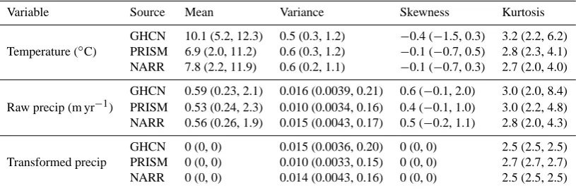
Table 2. Statistics of annual climate data for both temperature and precipitation. Results for precipitation are shown for both the raw data and

after the transformation to Gaussian, as described in the text. For each statistic, the median for all grid cells is listed followed by the 5th and 95th percentile values in parentheses. Note that a Gaussian distribution has a skewness of 0 and a kurtosis of 3, but that with smaller sample sizes a discrete approximation to a Gaussian results in slightly lower values for the kurtosis.

Variable Source Mean Variance Skewness Kurtosis

GHCN 10.1 (5.2, 12.3) 0.5 (0.3, 1.2) −0.4 (−1.5, 0.3) 3.2 (2.2, 6.2) Temperature (◦C) PRISM 6.9 (2.0, 11.2) 0.6 (0.3, 1.2) −0.1 (−0.7, 0.5) 2.8 (2.3, 4.1) NARR 7.8 (2.2, 11.9) 0.6 (0.2, 1.1) −0.1 (−0.7, 0.3) 2.7 (2.0, 4.0)

GHCN 0.59 (0.23, 2.1) 0.016 (0.0039, 0.21) 0.6 (−0.1, 2.0) 3.0 (2.0, 8.4) Raw precip (m yr−1) PRISM 0.53 (0.24, 2.3) 0.010 (0.0034, 0.16) 0.4 (−0.1, 1.0) 3.0 (2.2, 4.8) NARR 0.56 (0.26, 1.9) 0.015 (0.0043, 0.17) 0.5 (−0.2, 1.1) 2.8 (2.0, 4.3)

GHCN 0 (0, 0) 0.015 (0.0036, 0.20) 0 (0, 0) 2.5 (2.5, 2.5) Transformed precip PRISM 0 (0, 0) 0.010 (0.0033, 0.15) 0 (0, 0) 2.7 (2.7, 2.7) NARR 0 (0, 0) 0.014 (0.0043, 0.16) 0 (0, 0) 2.5 (2.5, 2.5)

obtained from the National Climatic Data Center (NCDC; http://nomads.ncdc.noaa.gov/). GHCN is an integrated and quality-assured database of land surface stations (Lawrimore et al., 2011; stations included in the present analysis are listed in Table A1). Daily data were quality controlled by elimi-nating any temperature excursions that exceeded 5 standard deviations of all daily measurements for a specific calen-dar month, and any daily precipitation measurements that exceeded 254 mm (10 inches). Annual averages of GHCN observations were compiled from daily data by requiring a minimum of 10 days to compute a monthly average and 9 months to compute an annual average – different choices for these thresholds did not substantially impact the results. The 181 stations with complete records for 1979–2011 were included in the analysis.

Before proceeding, we assess the extent to which the data satisfy the two assumptions listed in the previous section, which are necessary conditions for applying the ensemble sensitivity approach. The first assumption, linearity, is not an issue for our application: since we intend to model pre-cipitation and temperature using distributed observations of precipitation and temperature, our model simply consists of an average and is therefore linear.

The assumption of Gaussian statistics is worth investigat-ing in some depth, in particular with regard to precipitation, which – even at annual timescales – exhibits a distribution that is skewed toward larger values. Table 2 lists the statis-tics of temperature, raw precipitation, and transformed pre-cipitation data, showing the range of each statistic over all

grid points. The transformed precipitation was created by remapping the observed cumulative distribution of precipita-tion to that of a normal distribuprecipita-tion (by matching quantiles). To preserve the spatial variability in precipitation, the width of the normal distribution was scaled to match the variance of the observations. The transformation was performed sep-arately for each grid cell since, although lumping all of the data together would improve sampling, it would not guaran-tee Gaussian statistics at each point. As can be seen in Ta-ble 2, the main impact of the precipitation transform is to eliminate any skewness in the data, though it is notable that the raw precipitation data is very nearly Gaussian as well. For this reason, our default in the calculations below is to use raw precipitation, though we note the impact of using trans-formed precipitation in the sensitivity tests discussed below.

2.3 Measurement error

(5)

average temperature. A constant value forR2 is applied to all grid cells. Since measurements of precipitation are not generally assimilated in weather forecasting, there does not exist a similar estimate for the appropriate error variance in precipitation. As a result, we estimate the error variance for precipitation by simply rescaling the value used for temper-ature using the ratio of the variance in precipitation to the variance in temperature, and accounting for a precipitation autocorrelation timescale of 2 days instead of 5. This cor-responds to an error variance of∼3.6 % of the variance in precipitation at each grid cell and a median error variance of 375 mm2(for total annual precipitation). Note that this is an approximation, since precipitation measurements are sub-ject to different and often greater errors than for temperature. However, such differences are likely far less than the span of the sensitivity tests forR2, described below. Finally, note that in contrast with temperature,R2is scaled with the grid cell variance in precipitation, since using a constant error vari-ance would bias the results in favor of wetter regions.

Since both estimates ofR2 are approximations, we per-form two simple verifications: (1) using raw surface obser-vations from two nearby stations, and (2) using a gridded estimate of representativeness error. Note that in both cases we are assuming that the magnitude ofR2 is dominated by the representativeness error – a good assumption given that propagating the error in daily measurements of temperature and precipitation gives an annual instrument error of about 0.0001 K2and 0.01 mm2, respectively.

In the first approach we consider the mean-squared dif-ference between two nearby observing stations – Sea-Tac airport (47.45◦_{N, 122.3}◦_{W) and Kent COOP (47.4}◦_N,

122.2◦_{W) – for the overlapping time series spanning 1951–}

2011. The result is a value of 0.28 K2 for temperature and 7800 mm2 for precipitation. Our central estimate forR2at that location is ∼950 mm2 for precipitation (and, as with all grid cells, 0.05 K2 for temperature). Note that the dis-tance between these two observing stations is 7.5 km, which is about twice the grid resolution of the PRISM dataset, mak-ing it likely that these numbers represent an overestimate of representativeness error

Our second approach to verifying theR2estimates from ECMWF is to use the 30 arc-seconds (∼800 m resolution) climatologies available from PRISM to estimate the sub-grid variance in temperature and precipitation for each 2.5 arcmin (∼4 km) grid cell. This gives an estimate of the represen-tativeness error that varies with each grid cell, with a me-dian of 0.06 K2for temperature and 600 mm2for precipita-tion. The corresponding values from ECMWF are 0.05 K2 for temperature, and 375 mm2 for precipitation, indicating that as above, the ECMWF-based estimates are somewhat conservative but well within the range of our sensitivity tests, discussed below.

2.4 Sensitivity tests

As the above discussion of measurement error highlights, several of the parameters used in applying the method are uncertain. Specifically, in addition to measurement error, the method may be sensitive to the choice of climate dataset, precipitation transform, the number of years included in the gridded data, the sample size (in years) for each calcu-lation, and assumptions about the number of stations that the algorithm can meaningfully identify (i.e., as limited by sampling error). To address the sampling issues, we im-plemented a Monte Carlo routine in which the algorithm was run 50 000 times, using a different random sample of years for each iteration. The Monte Carlo approach also ad-dresses the question of noise limitations, since statistics can be obtained on the consistency of results between iterations (see discussion below). To test robustness to other parame-ters, we performed the following sensitivity tests: measure-ment error variance (R2) was scaled by a factor ranging from 0.1 to 10, calculations were repeated for different cli-mate datasets, precipitation transforms, sample sizes (rang-ing from 20 to 40 yr), and years from which to draw samples (1948–1979 vs. 1980–2011).

3 Results and discussion

Figure 2 shows the best estimate of the optimal observing locations, obtained using the following choices of data and parameters:

– metric (J): regionally averaged annual temperature and precipitation;

– dataset: PRISM;

– years: 1948–2011;

– sample size: 30 yr;

– R2= 0.05 K2for temperature;

– R2= 3.6 % of the grid cell variance in precipitation;

– precipitation: raw data (not transformed).

In this section we discuss these results along with the results of our sensitivity tests, which evaluate the impact of varying the above parameters and assumptions.

(6)

TEMP PRCP

50 75 90 95 99

Fig. 2. Results for annual temperature and precipitation, obtained using the optimal network design calculation. Calculations were performed

using regionally averaged temperature and precipitation as the target metric (defined as the average over the US states of Idaho, Oregon, and Washington). Contours show the percentile value of the grid cell weighting – higher weights denote areas where measurements contribute more to the variance explained. Results are obtained using the PRISM dataset (1948–2011), central estimates for the measurement error (R2), and a sample size of 30 yr.

Since these frequency values are most meaningful in a rel-ative sense – which grid cells have greater weightings than others – we display the percentile values of the grid cell weightings, which we consider more helpful for interpreta-tion. For example, a point is assigned a 95th percentile value if its frequency value – the fraction of Monte Carlo iterations in which it was selected in the top “N” points – is greater than or equal to that of 95 % of all other points. Finally, in this and subsequent maps stemming from gridded PRISM data, the results have been averaged from 2.5 arcmin (∼4 km) res-olution to 0.5 degree resres-olution. This smoothing is applied to aid in interpretation.

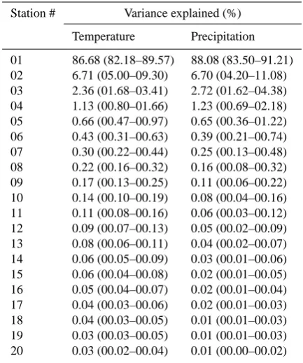
In order to choose “N” we look at the change in the vari-ance explained as the calculation progresses – in other words, the percent of the variance in the metric (regional tempera-ture or precipitation) that can be reproduced using a linear combination of the already-chosen stations. Table 3 lists the mean variance explained for both temperature and precipi-tation, for each additional station selection, for the results mapped in Fig. 2. As described in Sect. 2.1, the calcula-tion proceeds by selecting stacalcula-tions that maximize the residual variance explained – in other words, that maximize the addi-tional value lent by their selection. Table 3 illustrates that, due to high spatial autocorrelation across the region (in par-ticular at annual timescales), the first station explains a ma-jority of the variance, while subsequent stations account for progressively less of the residual variance. By summing the variance explained at each step, we find that, on average, the top 3 stations in temperature and the top 2 in precipitation are sufficient to explain 95 % of the variance in the annual climate signal for the PNW. Similarly, to explain 99 % of the variance would require selection of the top 11 and 4 stations for temperature and precipitation, respectively. For simplic-ity, we only show results for the former (i.e., 95 % variance

Table 3. Percent of the variance explained with each station

selec-tion. Values shown are the median and 5th–95th percentile values (in parentheses) based on all 50 000 Monte Carlo calculations.

Station # Variance explained (%)

Temperature Precipitation

01 86.68 (82.18–89.57) 88.08 (83.50–91.21) 02 6.71 (05.00–09.30) 6.70 (04.20–11.08) 03 2.36 (01.68–03.41) 2.72 (01.62–04.38) 04 1.13 (00.80–01.66) 1.23 (00.69–02.18) 05 0.66 (00.47–00.97) 0.65 (00.36–01.22) 06 0.43 (00.31–00.63) 0.39 (00.21–00.74) 07 0.30 (00.22–00.44) 0.25 (00.13–00.48) 08 0.22 (00.16–00.32) 0.16 (00.08–00.32) 09 0.17 (00.13–00.25) 0.11 (00.06–00.22) 10 0.14 (00.10–00.19) 0.08 (00.04–00.16) 11 0.11 (00.08–00.16) 0.06 (00.03–00.12) 12 0.09 (00.07–00.13) 0.05 (00.02–00.09) 13 0.08 (00.06–00.11) 0.04 (00.02–00.07) 14 0.06 (00.05–00.09) 0.03 (00.01–00.06) 15 0.06 (00.04–00.08) 0.02 (00.01–00.05) 16 0.05 (00.04–00.07) 0.02 (00.01–00.04) 17 0.04 (00.03–00.06) 0.02 (00.01–00.03) 18 0.04 (00.03–00.05) 0.01 (00.01–00.03) 19 0.03 (00.03–00.05) 0.01 (00.01–00.03) 20 0.03 (00.02–00.04) 0.01 (00.00–00.02)

explained) in Fig. 2 and all subsequent figures. The results for different choices are qualitatively similar.

(7)

other regions (see Fig. 1 for a key to the geography of the region). For precipitation, the results are quite different, pri-marily highlighting the central Cascades, the Columbia gorge near Portland, the southeastern slopes of the Olympic moun-tains in Washington, and certain parts of the coast of Ore-gon. Notably, the optimal locations for monitoring tempera-ture are almost entirely east of the Cascade mountains, while the opposite is true for the optimal observing locations iden-tified for precipitation. In addition, some of the results are quite counterintuitive. For instance, while it makes sense that precipitation monitoring will maximize signal to noise on the substantially wetter western slopes of the Cascade moun-tains, it is not intuitively obvious that the central Cascade mountains are more appropriate than any other portion of this mountain range, nor is it clear why the even wetter western slopes of the Olympic mountains are hardly highlighted at all.

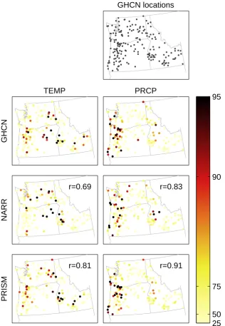
Figure 3 shows a comparison of results obtained from the three datasets: GHCN, NARR, and PRISM. In order to per-form a direct comparison, NARR and PRISM data were only used for the grid points that correspond most closely to the location of each GHCN station, and all datasets applied to the years 1979–2011 only, with a sample size of 20 yr for each calculation. TheR2 values applied to each case were iden-tical. Note that this is not a perfect comparison, since point measurements (i.e., GHCN) are different from grid-cell aver-ages (NARR, 32 km resolution; PRISM,∼4 km resolution). The rank correlations between the GHCN results and each gridded dataset are shown in the upper right-hand corner of each map. Since disagreement among adjacent stations could confound the results, we calculated correlations by first av-eraging the point results for each dataset onto a 0.5 degree grid. Point correlations (not shown) were significant but sub-stantially lower than their gridded counterparts. We use rank correlations because the results are highly skewed, causing standard correlations to be disproportionately affected by a small number of points. Since our emphasis in this work is on the relative rankings among grid points, we deem the rank correlations a better measure of similarities among the re-sults. Standard correlations also revealed significant positive correlations, but nonetheless lower values.

A number of observations can be made from these results. First, at coarse scales (i.e., the broad regions highlighted) there is good agreement among the three datasets. Second, PRISM and GHCN bear the greatest similarities, a fact which is perhaps not surprising given that PRISM is essentially a regridding of surface observations. Third, although the gen-eral picture remains consistent between datasets, the specific rankings can differ substantially (as reflected in the correla-tions). Since the three agree well at coarser spatial scales, this suggests that the discrepancies are primarily in the treat-ment of climate variations across smaller scales. We thus conclude that, until well-validated improvements in datasets become available, the results are best viewed as defining broad regions within which to focus efforts. Based on this

comparison, Fig. 2 and all subsequent results are shown us-ing the PRISM dataset, averaged to 0.5 degree resolution (i.e., calculations are performed at the native PRISM reso-lution of∼4 km, then averaged to 0.5 degree resolution for presentation).

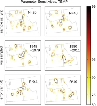
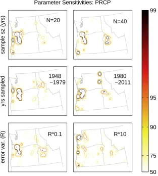
A primary advantage of our approach is that it is objective, and that it is therefore capable of highlighting non-intuitive but nonetheless optimal observing locations. However, im-plementation of the method does entrain a number of impor-tant subjective decisions, as highlighted at the beginning of this section. Figures 4 and 5 show how the results are affected by varying the parameters chosen for the calculation. Specif-ically, we test for the influence of variations in the sample size (20 vs. 40 yr), the years from which to draw a sample (1948–1979 vs. 1980–2011), and the value for the total er-ror variance (R2; 10 times smaller vs. 10 times larger than our central estimate) in temperature (Fig. 4) and precipita-tion (Fig. 5). Note that changing the values ofR2 changes the number of stations (“N”) needed to achieve 95 % vari-ance explained – these were adjusted accordingly in the maps showing sensitivity toR2. Note, also, that we do not consider variations in the metric (J) – this would by definition alter the results, but would not inform our question regarding the robustness of the method.

Overall, as with Fig. 3, these results show broad consisten-cies across different parameter values, highlighting similar areas for monitoring despite large variations in parameters. Precipitation results appear to be much more robust than those for temperature. For both variables, the results are largely insensitive to the choice of sample size, but indi-cate a fair sensitivity to the choice of years sampled and, in particular, to R2. The magnitude of R2 impacts the extent to which the correlation withJ is balanced by the ratio of signal-to-noise: small values forR2 favor areas that corre-late best with the regional signal, while large values ofR2 favor areas with higher variance. Even in the case ofR2, it is notable that the dominant regions highlighted nearly always correspond to regions that are also highlighted in Fig. 2.

(8)

GHCN locations

GHCN

TEMP

r=0.69

NARR

r=0.81

PRISM

PRCP

r=0.83

r=0.91

25

50

75

90

95

Fig. 3. Results from three different datasets (GHCN, NARR, PRISM), calculated for the 181 GHCN stations with continuous records for the

period 1979–2011. The top map, labeled “GHCN locations”, shows the location of the GHCN stations used in the calculation. The 6 other maps show results for the different datasets. Each dot denotes the location of a GHCN station, and is shaded according to the percentage of time the station was chosen using the network design algorithm. Rank correlations with the GHCN results are shown in the top right corner of the NARR and PRISM maps. As with Fig. 2, percentile values are plotted to simplify interpretation. Note that, unlike in other figures, the color scale remains a light yellow at low values, and does not fade to white.

4 Conclusions

The ensemble sensitivity approach provides an objective method for allocating resources to develop an observational network. It allows for rapid evaluation of different metrics, and requires only a climatological sample. Since the utility of each observation is maximized, optimal placement ensures an efficient use of resources. There are two salient features to

the approach: (1) stations are selected based on a compro-mise between their correlation with the metric and the ratio of signal-to-noise, and (2) new selections are constrained to minimize redundancy by maximizing the additional variance explained.

(9)

sample sz (yrs)

Parameter Sensitivities: TEMP

N=20

_N=40

yrs sampled

1948

−1979

1980

−2011

error var. (R)

R*0.1

R*10

50

75

90

95

99

Fig. 4. Sensitivity of network design results for annual temperature, obtained by varying the parameters used to apply the algorithm. The top

row shows results in which the sample size is varied between 20 and 40 yr, the middle row shows results obtained from the first half of the record (1948–1979) and the last half (1980–2011), and the bottom row shows the impact of scaling the measurement error (R2) by an order of magnitude in each direction.

10 optimally placed stations. We find that station placement is not intuitive, highlighting the importance of employing objective methods for network design. Note that this infor-mation can be used in one of two ways: (1) install only 5–10 new observing stations instead of the total number planned, or (2) pursue other monitoring goals (e.g., monitor-ing sub-regional climate(s), seasonal climate, or probability of extremes).

Sensitivity tests indicate that the results are robust to the choice of sample size and time period analyzed, but that there are important differences resulting from the choice of dataset and assumed measurement error (R2). Sensitiv-ity toR2 is fairly strong, but in general does not result in the identification of new regions for monitoring. Differences among datasets are likely partially attributable to differences in spatial resolution and the distinction between point mea-surements and grid cell averages. However, it is also likely that these differences represent real differences in the mod-eled covariability of temperature and precipitation across the

region. Fortunately, the differences among datasets largely result from small spatial scale distinctions between each: the broad-scale patterns are consistent. Since important differ-ences do exist, we conclude that until an improved dataset becomes available, the method is best used to identify gen-eral areas in which to locate stations. In practice, this is un-likely to be a limitation, since siting decisions at local scales are dominated by practical constraints such as land owner-ship, access, etc.

(10)

sample sz (yrs)

Parameter Sensitivities: PRCP

N=20

_N=40

yrs sampled

1948

−1979

1980

−2011

error var. (R)

R*0.1

R*10

50

75

90

95

99

Fig. 5. As in Fig. 4 except applied to annual precipitation.

west, temperatures in the interior will still be more variable than at the coasts, etc. – we do not believe that this is a ma-jor concern. Furthermore, the assumption that the statistical relationships will remain the same with a changing climate is common in climate research (e.g., statistical downscaling, paleoclimate reconstructions). Moreover, an alternative ap-proach, such as using GCM simulations, would have its own set of caveats in this regard (bias, coarse resolution, etc.).

A primary advantage of the ensemble sensitivity method is that it can be modified in a way that takes into account practi-cal and scientific considerations while ensuring that the net-work maximizes return on investment. For instance, there are important practical constraints on station siting, such as land ownership, proximity to roads, and the presence of existing stations. These are easily incorporated into the calculations by (a) constraining the first “n” station selections to corre-spond to existing observations, and (b) simply masking out grid cells that do not conform to the selection criteria. Fur-thermore, climatological networks are not designed to mon-itor just one quantity, and it is not necessarily the case that sites that capture a large fraction of the variance in precipita-tion should also be useful for monitoring other variables. The

method could be made to iteratively select temperature and precipitation stations, making each conditional on the other. Flexibility is a key advantage of this approach: it can be eas-ily adapted to the practical constraints of station siting while still ensuring that the monitoring goals are pursued optimally. There are numerous potential applications for the ensem-ble sensitivity method spanning multiple fields, monitoring goals, and regions of interest. The advantage of optimal de-sign is that it ensures an efficient use of resources. We believe that this approach can be a useful tool for informing decisions in network design.

Acknowledgements. Funding for this research was provided in part

by NSF Grant 1043090, as well as the State of Washington through funding to the Office of Washington State Climatologist.

(11)

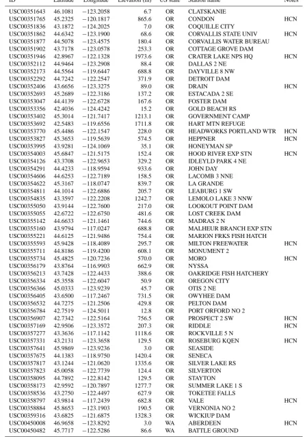
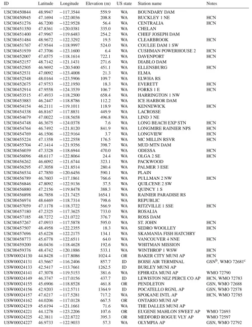
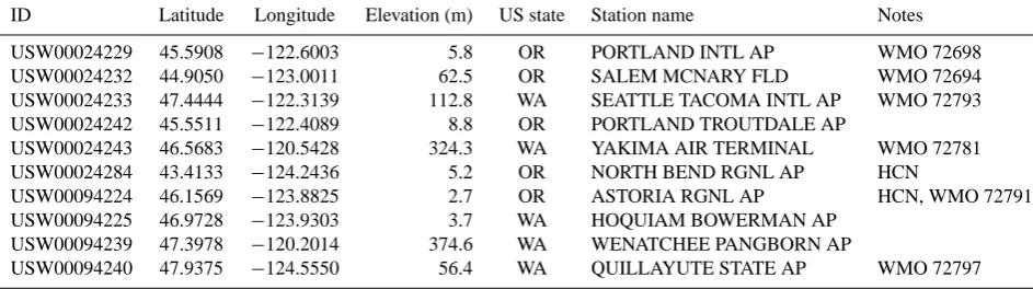
Table A1. GHCN station attributes.

ID Latitude Longitude Elevation (m) US state Station name Notes

USC00100010 42.9536 −112.8253 1342.6 ID ABERDEEN EXP STN HCNa USC00100667 47.9803 −116.5594 636.1 ID BAYVIEW MODEL BASIN

USC00101017 43.7383 −116.2022 1184.1 ID BOISE 7 N

USC00101018 43.5253 −116.0542 865.6 ID BOISE LUCKY PEAK DAM USC00101220 42.6006 −114.7453 1158.2 ID BUHL #2

USC00101363 48.0864 −116.0572 662.3 ID CABINET GORGE

USC00101408 44.5733 −116.6753 807.7 ID CAMBRIDGE HCN

USC00101514 44.5228 −116.0481 1492.3 ID CASCADE 1 NW USC00101551 42.5503 −114.8661 1165.9 ID CASTLEFORD 2 N USC00101671 43.9772 −113.8289 1908.0 ID CHILLY BARTON FLAT USC00102260 43.4650 −113.5581 1797.4 ID CRATERS OF THE MOON USC00102444 43.5764 −116.7475 765.0 ID DEER FLAT DAM USC00102707 44.2436 −112.2006 1661.2 ID DUBOIS EXP STN

USC00102845 46.5022 −116.3217 303.3 ID DWORSHAK FISH HATCH HCN USC00102875 45.8356 −115.4611 1236.9 ID ELK CITY 1NE

USC00102942 43.8544 −116.4664 728.5 ID EMMETT 2 E

USC00103143 46.0931 −115.5356 475.5 ID FENN RS HCN

USC00103297 43.0428 −112.4133 1360.9 ID FT HALL 1 NNE

USC00103631 42.9403 −115.3231 751.6 ID GLENNS FERRY HCN USC00103771 45.9414 −116.1175 1005.8 ID GRANGEVILLE

USC00103964 43.9664 −112.2642 1460.0 ID HAMER 4 NW

USC00104140 42.5972 −114.1378 1237.5 ID HAZELTON HCN

USC00104295 42.3528 −114.5739 1379.2 ID HOLLISTER HCN

USC00104384 43.7828 −113.0033 1469.1 ID HOWE USC00104442 43.8383 −115.8319 1208.5 ID IDAHO CITY USC00104456 43.3456 −111.7847 1776.4 ID IDAHO FALLS 16 SE

USC00104670 42.7325 −114.5192 1140.0 ID JEROME HCN

USC00104831 47.5339 −116.1222 724.5 ID KELLOGG HCN

USC00104845 43.6842 −114.3603 1795.3 ID KETCHUM RS HCN

USC00105275 42.1231 −111.3139 1806.2 ID LIFTON PUMPING STN HCN USC00105708 44.8872 −116.1047 1531.6 ID MC CALL

USC00105897 44.7189 −115.0150 1365.5 ID MIDDLE FORK LODGE

USC00106152 46.7281 −116.9558 810.8 ID MOSCOW U OF I HCN USC00106305 43.6039 −116.5753 752.9 ID NAMPA SUGAR FACTORY HCN

USC00106542 42.2342 −113.8981 1389.6 ID OAKLEY HCN

USC00106844 43.8022 −116.9442 698.0 ID PARMA EXP STN

USC00106891 44.0764 −116.9311 655.3 ID PAYETTE HCN

USC00107040 43.3111 −114.0742 1472.2 ID PICABO USC00107046 46.4922 −115.8006 938.8 ID PIERCE USC00107320 46.5100 −114.7111 1075.9 ID POWELL

USC00107386 48.3511 −116.8353 722.7 ID PRIEST RIVER EXP STN HCN USC00107648 43.2064 −116.7494 1197.9 ID REYNOLDS

USC00108022 43.9517 −111.6789 1496.6 ID SAINT ANTHONY

USC00108080 45.1875 −113.9008 1198.2 ID SALMON−KSRA HCN USC00108380 42.9383 −114.4169 1204.0 ID SHOSHONE 1 WNW

USC00108928 43.2436 −116.3783 708.7 ID SWAN FALLS P H USC00108937 43.4447 −111.2939 1633.7 ID SWAN VALLEY 2 E USC00109065 43.8564 −111.2769 1880.6 ID TETONIA EXP STN USC00109303 42.5458 −114.3461 1207.0 ID TWIN FALLS 6 E USC00109846 46.2381 −116.6233 1210.7 ID WINCHESTER

USC00350304 42.2128 −122.7144 532.2 OR ASHLAND HCN

USC00350471 43.1497 −124.4019 6.1 OR BANDON 2 NNE USC00350652 44.2867 −122.0386 655.9 OR BELKNAP SPRINGS 8 N

USC00350694 44.0567 −121.2850 1115.6 OR BEND HCN

USC00350897 45.6361 −121.9519 18.9 OR BONNEVILLE DAM

USC00351433 44.3914 −122.4811 292.6 OR CASCADIA HCN

(12)

Table A1. Continued.

USC00351643 46.1081 −123.2058 6.7 OR CLATSKANIE

USC00351765 45.2325 −120.1817 865.6 OR CONDON HCN

USC00351836 43.1872 −124.2025 7.0 OR COQUILLE CITY

USC00351862 44.6342 −123.1900 68.6 OR CORVALLIS STATE UNIV HCN USC00351877 44.5078 −123.4575 180.4 OR CORVALLIS WATER BUREAU

USC00351902 43.7178 −123.0578 253.3 OR COTTAGE GROVE DAM

USC00351946 42.8967 −122.1328 1973.6 OR CRATER LAKE NPS HQ HCN USC00352112 44.9464 −123.2908 88.4 OR DALLAS 2 NE

USC00352173 44.5564 −119.6447 688.8 OR DAYVILLE 8 NW USC00352292 44.7242 −122.2547 371.9 OR DETROIT DAM

USC00352406 43.6656 −123.3275 89.0 OR DRAIN HCN

USC00352693 45.2689 −122.3186 137.2 OR ESTACADA 2 SE USC00353047 44.4139 −122.6728 167.6 OR FOSTER DAM USC00353356 42.4036 −124.4242 15.2 OR GOLD BEACH RS USC00353402 45.3014 −121.7417 1213.1 OR GOVERNMENT CAMP USC00353692 42.5483 −119.6556 1711.8 OR HART MTN REFUGE

USC00353770 45.4486 −122.1547 228.0 OR HEADWORKS PORTLAND WTR HCN

USC00353827 45.3653 −119.5639 574.5 OR HEPPNER HCN

USC00353995 43.9281 −124.1069 35.1 OR HONEYMAN SP

USC00354003 45.6847 −121.5175 152.4 OR HOOD RIVER EXP STN HCN USC00354126 43.3708 −122.9653 329.2 OR IDLEYLD PARK 4 NE

USC00354291 44.4233 −118.9594 933.6 OR JOHN DAY USC00354606 44.6253 −122.7189 158.5 OR LACOMB 3 NNE USC00354622 45.3167 −118.0747 839.7 OR LA GRANDE USC00354811 44.1014 −122.6886 205.7 OR LEABURG 1 SW USC00354835 43.3597 −122.2208 1242.7 OR LEMOLO LAKE 3 NNW USC00355050 43.9144 −122.7600 217.0 OR LOOKOUT POINT DAM USC00355055 42.6722 −122.6750 481.6 OR LOST CREEK DAM USC00355142 44.6633 −121.1461 744.6 OR MADRAS 2 N

USC00355160 43.9794 −117.0247 688.8 OR MALHEUR BRANCH EXP STN USC00355221 44.6125 −121.9486 754.4 OR MARION FRKS FISH HATCH

USC00355593 45.9428 −118.4089 295.7 OR MILTON FREEWATER HCN USC00355711 44.8186 −119.4200 608.1 OR MONUMENT 2

USC00355734 45.4825 −120.7236 570.0 OR MORO HCN

USC00356179 43.8764 −116.9903 662.9 OR NYSSA

USC00356213 43.7428 −122.4433 388.6 OR OAKRIDGE FISH HATCHERY USC00356334 45.3558 −122.6047 50.9 OR OREGON CITY

USC00356366 45.0333 −123.9239 45.7 OR OTIS 2 NE USC00356405 43.6500 −117.2467 731.5 OR OWYHEE DAM USC00356532 44.7275 −121.2506 429.8 OR PELTON DAM USC00356784 42.7519 −124.5011 12.8 OR PORT ORFORD NO 2

USC00356907 42.7342 −122.5164 756.5 OR PROSPECT 2 SW HCN

USC00357169 42.9506 −123.3572 207.3 OR RIDDLE HCN

USC00357277 43.3636 −117.1142 1118.6 OR ROCKVILLE 5 N

USC00357331 43.2131 −123.3658 129.5 OR ROSEBURG KQEN HCN

USC00357641 45.9869 −123.9236 3.0 OR SEASIDE USC00357675 44.1383 −118.9750 1420.4 OR SENECA

USC00357817 43.1244 −121.0620 1335.6 OR SILVER LAKE RS USC00357823 45.0058 −122.7739 124.4 OR SILVERTON USC00358095 44.7892 −122.8142 129.5 OR STAYTON

USC00358173 42.9592 −120.7897 1277.7 OR SUMMER LAKE 1 S USC00358536 43.2750 −122.4497 627.9 OR TOKETEE FALLS

USC00358797 43.9814 −117.2439 682.8 OR VALE HCN

USC00358884 45.8653 −123.1903 190.5 OR VERNONIA NO 2 USC00359316 43.6825 −121.6875 1328.3 OR WICKIUP DAM

USC00450008 46.9658 −123.8292 3.0 WA ABERDEEN HCN

(13)

USC00450844 48.9947 −117.3544 559.9 WA BOUNDARY DAM

USC00450945 47.1694 −122.0036 208.8 WA BUCKLEY 1 NE HCN

USC00451276 46.7200 −122.9528 56.4 WA CENTRALIA HCN

USC00451350 47.8361 −120.0381 335.0 WA CHELAN

USC00451400 47.9967 −119.6483 254.2 WA CHIEF JOSEPH DAM

USC00451484 48.9672 −122.3292 19.5 WA CLEARBROOK HCN

USC00451767 47.9544 −118.9997 524.0 WA COULEE DAM 1 SW

USC00451939 47.3706 −123.1600 6.4 WA CUSHMAN POWERHOUSE 2 HCN

USC00452007 47.6575 −118.1614 722.1 WA DAVENPORT HCN

USC00452157 48.7142 −121.1431 271.6 WA DIABLO DAM

USC00452505 46.9692 −120.5400 451.1 WA ELLENSBURG HCN

USC00452531 47.0092 −123.4008 21.3 WA ELMA USC00452548 48.0164 −123.5906 109.7 WA ELWHA RS

USC00452675 47.9753 −122.1950 18.3 WA EVERETT HCN

USC00452914 47.9558 −124.3539 106.7 WA FORKS 1 E HCN

USC00453515 47.4933 −118.2500 658.4 WA HARRINGTON 1 NW USC00453883 46.2447 −118.8786 112.2 WA ICE HARBOR DAM

USC00454154 46.2111 −119.1011 118.9 WA KENNEWICK HCN

USC00454338 46.8167 −117.8831 449.9 WA LACROSSE USC00454679 47.0022 −118.5658 496.8 WA LIND 3 NE

USC00454748 46.3675 −124.0378 7.6 WA LONG BEACH EXP STN HCN USC00454764 46.7492 −121.8120 841.9 WA LONGMIRE RAINIER NPS HCN

USC00454769 46.1506 −122.9164 3.7 WA LONGVIEW HCN

USC00455224 47.1358 −122.2558 176.5 WA MC MILLIN RSVR HCN USC00455704 47.1414 −121.9356 398.7 WA MUD MTN DAM

USC00456039 47.3328 −118.6944 470.0 WA ODESSA HCN

USC00456096 48.6117 −122.8064 24.4 WA OLGA 2 SE HCN

USC00456262 46.6092 −121.6744 323.1 WA PACKWOOD USC00456295 47.3058 −121.8514 280.4 WA PALMER 3 ESE USC00456534 47.7850 −120.6456 590.1 WA PLAIN

USC00456789 46.7603 −117.1861 766.6 WA PULLMAN 2 NW HCN

USC00456846 47.8092 −122.9136 37.5 WA QUILCENE 2 SW USC00456880 47.2156 −119.8478 388.3 WA QUINCY 1 S

USC00456898 46.7858 −121.7425 1654.1 WA RAINIER PARADISE RS USC00456974 48.6469 −118.7314 798.6 WA REPUBLIC

USC00457059 47.1178 −118.3722 566.9 WA RITZVILLE 1 SSE HCN USC00457180 47.2325 −117.3625 733.0 WA ROSALIA

USC00457185 48.7272 −121.0722 376.7 WA ROSS DAM

USC00457267 47.0933 −117.5878 595.0 WA ST. JOHN HCN

USC00457507 48.4958 −122.2355 18.3 WA SEDRO WOOLLEY HCN

USC00457696 45.6228 −122.2175 134.1 WA SKAMANIA FISH HATCHRY

USC00458773 45.6778 −122.6511 64.0 WA VANCOUVER 4 NNE HCN USC00459200 46.0436 −118.4628 192.6 WA WHITMAN MISSION

USC00459376 48.4742 −120.1886 533.1 WA WINTHROP 1 WSW HCN USW00024130 44.8428 −117.8086 1024.4 OR BAKER CITY MUNI AP HCN

USW00024131 43.5667 −116.2406 857.7 ID BOISE AIR TERMINAL GSNb, WMO 72681c USW00024133 42.5417 −113.7661 1262.5 ID BURLEY MUNI AP

USW00024141 47.3078 −119.5153 381.6 WA EPHRATA MUNI AP WMO 72790 USW00024149 46.3747 −117.0156 437.7 ID LEWISTON NEZ PERCE CO AP HCN, WMO 72783

USW00024155 45.6906 −118.8528 461.8 OR PENDLETON GSN, WMO 72688

USW00024156 42.9203 −112.5711 1364.9 ID POCATELLO RGNL AP GSN, WMO 72578 USW00024157 47.6217 −117.5281 717.2 WA SPOKANE INTL AP HCN, WMO 72785 USW00024162 44.0206 −117.0128 667.5 OR ONTARIO MUNI AP

USW00024219 45.6194 −121.1661 71.6 WA THE DALLES MUNI AP

USW00024221 44.1278 −123.2206 107.6 OR EUGENE MAHLON SWEET AP WMO 72693 USW00024225 42.3811 −122.8722 395.3 OR MEDFORD ROGUE VLY AP WMO 72597

(14)

USW00024229 45.5908 −122.6003 5.8 OR PORTLAND INTL AP WMO 72698 USW00024232 44.9050 −123.0011 62.5 OR SALEM MCNARY FLD WMO 72694 USW00024233 47.4444 −122.3139 112.8 WA SEATTLE TACOMA INTL AP WMO 72793 USW00024242 45.5511 −122.4089 8.8 OR PORTLAND TROUTDALE AP

USW00024243 46.5683 −120.5428 324.3 WA YAKIMA AIR TERMINAL WMO 72781 USW00024284 43.4133 −124.2436 5.2 OR NORTH BEND RGNL AP HCN

USW00094224 46.1569 −123.8825 2.7 OR ASTORIA RGNL AP HCN, WMO 72791 USW00094225 46.9728 −123.9303 3.7 WA HOQUIAM BOWERMAN AP

USW00094239 47.3978 −120.2014 374.6 WA WENATCHEE PANGBORN AP

USW00094240 47.9375 −124.5550 56.4 WA QUILLAYUTE STATE AP WMO 72797

a_{indicates the station is included in the US Historical Climatology Network (HCN);}b_{indicates the station is included in the Global Climate Observing System (GCOS)} Surface Network (GSN);cdenotes the Word Meteorological Organization (WMO) number for the station.

References

Abatzoglou, J., Redmond, K., and Edwards, L.: Classification of re-gional climate variability in the state of California, J. Appl. Me-teorol., 48, 1527–1541, doi:10.1175/2009JAMC2062.1, 2009. Ancell, B. and Hakim, G.: Comparing Adjoint-and

Ensemble-Sensitivity Analysis with Applications to Observa-tion Targeting, Mon. Weather Rev., 135, 4117–4134, doi:10.1175/2007MWR1904.1, 2007.

Bergot, T., Hello, G., Joly, A., and Malardel, S.: Adaptive Obser-vations: A Feasibility Study, Mon. Weather Rev., 127, 743–765, 1999.

Bishop, C. and Toth, Z.: Ensemble transformation and adaptive observations, J. Atmos. Sci., 56, 1748–1765, doi:10.1175/1520-0469(1999)056<1748:ETAAO>2.0.CO;2, 1999.

Dabberdt, W. and Schlatter, T.: Research opportunities from emerg-ing atmospheric observemerg-ing and modelemerg-ing capabilities, B. Am. Meteorol. Soc., 77, 305–323, 1996.

Daly, C., Gibson, W., Taylor, G., Johnson, G., and Pasteris, P.: A knowledge-based approach to the statistical mapping of climate, Clim. Res., 22, 99–113, 2002.

Fujioka, F.: A method for designing a fire weather network, J. At-mos. Ocean. Tech., 3, 564–570, 1986.

Hamill, T.: Ensemble-based atmospheric data assimilation, Cam-bridge Univ. Press, New York, 124–156, 2006.

Hargrove, W., Hoffman, F., and Law, B.: New analysis reveals rep-resentativeness of the AmeriFlux network, Eos, 84, 529–535, 2003.

Huntley, H. and Hakim, G.: Assimilation of time-averaged obser-vations in a quasi-geostrophic atmospheric jet model, Clim. Dy-nam., 35, 995–1009, doi:10.1007/s00382-009-0714-5, 2010.

Kalman, R.: A new approach to linear filtering and prediction prob-lems, J. Basic Eng., 82, 35–45, 1960.

Khare, S. and Anderson, J.: A methodology for fixed observational network design: theory and application to a simulated global pre-diction system, Tellus A, 58, 523–537, 2006.

Lawrimore, J. H., Menne, M. J., Gleason, B. E., Williams, C. N., Wuertz, D. B., Vose, R. S., and Rennie, J.: An overview of the Global Historical Climatology Network monthly mean tempera-ture data set, version 3 (1984–2012), J. Geophys. Res.-Atmos., 116, D19121, doi:10.1029/2011JD016187, 2011.

Lundquist, J. and Cayan, D.: Surface temperature patterns in com-plex terrain: Daily variations and long-term change in the cen-tral Sierra Nevada, California, J. Geophys. Res., 112, D11124, doi:10.1029/2006JD007561, 2007.

Mesinger, F., DiMego, G., Kalnay, E., Mitchell, K., Shafran, P., Ebisuzaki, W., Jovic, D., Woollen, J., Rogers, E., Berbery, E., Ek, M., Fan, Y., Grumbine, R., Higgins, W., Li, H., Lin, Y., Manikin, G., Parrish, D., and Shi, W.: North American regional reanalysis, B. Am. Meteorol. Soc., 87, 343–360, doi:10.1175/BAMS-87-3-343, 2006.

Morss, R., Emanuel, K., and Snyder, C.: Idealized adaptive obser-vation strategies for improving numerical weather prediction, J. Atmos. Sci., 58, 210–232, 2001.