Measuring performance of a hybrid system based on imprecise data: Modeling and solution approaches

(1)

Journal of Industrial Engineering and Management Studies

Vol. 6, No. 2, 2019, pp. 214-239 DOI: 10.22116/JIEMS.2019.94192

www.jiems.icms.ac.ir

Measuring performance of a hybrid system based on imprecise

data: Modeling and solution approaches

Ehsan Vaezi1, Seyyed Esmaeil Najafi1,*, Mohammad Hadji Molana1, Farhad Hosseinzadeh Lotfi2, Mahnaz Ahadzadeh Namin3

Abstract

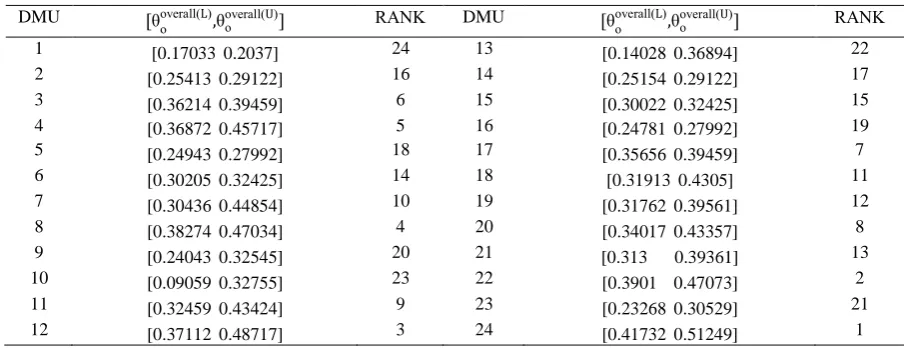
Data Envelopment Analysis (DEA) is one of the methods most widely used for measuring the relative efficiency of DMUs in the world today. The efficiency evaluation of the network structure opens the “black box” and considers the internal structure of systems. In this paper, a three-stage network model is considered with additional inputs and undesirable outputs and obtains the efficiency of the network, as interval efficiency in presence of the imprecise datum. The proposed model of this paper simulates a factory in the factual world with a production area, three warehouses and two delivery points. This factory is taken into consideration as a dynamic network and a multiplicative DEA approach is utilized to measure efficiency. Given the non-linearity of the models, a heuristic method is used to linearize the models. Ultimately, this paper concentrates on the interval efficiency to rank the units. The results of this ranking demonstrated that the time periods namely, (24) and (1) were the best and the poorest periods, respectively, in context to the interval efficiency within 24 phases of time.

Keywords: Network DEA; Three-stage processes; Interval data; Additional inputs; Undesirable outputs; minimax regret-based approach.

Received: January 2019-06 Revised: August 2019-05 Accepted: October 2019-07

1. Introduction

Evaluation and the measurement of performance will lead to smart or intelligent systems with incentives for individuals for the desired behavior. A measurement of performance is one of the fundamental managerial processes, for analyzing one’s own performance and likewise, surveying the conformity between the performance and the set of goals. The outcome of the evaluation can provide the grounds for taking the correct measures in decision-making for the future. Performance appraisal is a key part in the formulation and implementation of organizational policies (Hajijabbari & Sarabadani, 2008).

* Corresponding author; [email protected]

1_{Department of Industrial Engineering, Science and Research Branch, Islamic Azad University, Tehran, Iran.} 2_{Department of Mathematics, Science and Research Branch, Islamic Azad University, Tehran, Iran.}

(2)

The data envelopment analysis (DEA) is utilized as a non-parametric mathematical programming method, to evaluate the relative efficiency of entities, capable of being compared to multiple inputs and several outputs. These comparable entities are called decision-making units (DMUs). (Khalili-Damghani et al., 2015). Farrell (1957) considered a model for performance evaluation with an input and an output for the first time. Charnes, Cooper and Rhodes developed Farrell’s model for multiple inputs and outputs and dubbed it as “CCR” in honor of its makers (Charnes et al., 1978). Charnes, Cooper and Banker extended the DEA models and registered this model as their own and known as “BCC” (Banker et al., 1984). A failure to consider the internal correlations and the intermediate variables of complex systems (i.e. two or multiple stage processes), was a major flaw or defect, which the classic DEA models, such as, the CCR and BCC were labeled with. In actual fact, these models considered the systems as black boxes and would only be satisfied with the initial inputs and final outputs (Tone and Tsutsui, 2009). In order to overcome this problem, Fare and Grosskopf (2000) introduced the Network Data Envelopment Analysis (NDEA) models. With the assistance of the sub-series and parallels, including the intermediate variables, complex systems were simulated and a more genuine evaluation was computed (Chen and Yan, 2011). From Kao’s viewpoint, NDEA models can be categorized into three groups, namely, series, parallel and hybrid models. When the activities of a system are prolonged in respect to each other, the network has a serial structure; and at times when the activities are parallel to each other, the network has a parallel structure. Similarly, it maintains a hybrid mode, when there is a combination between the series and parallel set-up (Kao, 2009). Generally, the multiplicative and additive approaches are used to compute the network performance in the parallel and serial mode, respectively, (kao, 2006). After introducing the NDEA models, numerous studies took place in this field; and a combination of this science with branches of the game theory, brought about NDEA studies in cooperative and non-cooperative modes, which can be mentioned as hereunder. Li et al. (2012) presented a model for a two-stage structure, a phase which holds a more important standpoint for managers; and they have named this phase as “leader” and the other is known as “follower”. In order to calculate the efficiency, initially, the efficiency of the leader phase was maximized to the optimum and thus, the efficiency of the follower phase was secured by maintaining a constant efficiency in the phase of the leader. This exemplary, was designated as a decentralized control or a Stackelberg Game, which has been widely utilized by researchers in recent years. Du et al. (2015) analyzed a parallel network in the cooperative and non-cooperative modes and stated that, the efficiency of the former was more than that of the latter mode. An et al. (2017) considered a network, comprising of two stages, which interacted with each other; and computed the efficiency of this network in a cooperative and non-cooperative mode or condition. In another research Zhou et al. (2018), evaluated a multi-stage network in the non-cooperative and black box mode and compared the results. In recent years, the Stackelberg Game was utilized by several researchers such as, Fard and Hajaghaei-Keshteli (2018), Fard et al. (2018), including Hajaghaei-Hajaghaei-Keshteli and Fathollahi-Fard (2018).

(3)

was handled by imposing a single downward conversion. In the past few years, the role of the undesirable factors in DEA models has made considerable progress and the tasks of Wang et al. (2013) and Wu et al. (2016) are significant in this respect.

Classic DEA models, such as, (CCR and BCC models), were proposed for certainty in data as it does not deal with datum uncertainty. In fact, the actual, fundamental assumption in these models is that the amount of data in relevance with the inputs and outputs is an accurate numerical value. Though, in most cases, in the business environment, determining values for inputs and outputs is not feasible in reality (Khalili-Damghani et al., 2015). Ben-Tal and Nemirovski (2000), have demonstrated that an extremely slight deviation in the data leads to an unjustified response or a considerable change in the efficiency results. Hence, they proclaimed that the results of the classical DEA methods with determined parameters are not reliable. Kao (2006) stated that the reason for the absence of the presence of reliability, in terms of human judgment and concept, DEA models with imprecise data can play a more important role in evaluating efficiency in factual issues. Wang et al. (2009) expressed that in the presence of imprecise data, DEA models are capable of drawing insights for companies in variable and ambiguous conditions, in order to have a more realistic assessment of their own. Thereby, it is extremely essential to consider the uncertainty in the data available and the manner of dealing with it during the evaluation of efficiency by utilizing DEA methods. In most of the initial DEA tasks, uncertainty was ignored, but in recent years, several models have been under discussion for imprecise or inaccurate data (Azizi, 2013). Cooper et al. (1999) utilized a technique for DEA to confront imprecise data. Cooper et al. (2001) developed a method for converting a nonlinear planning problem into linear programming, by taking the alternative variables into consideration for determining the efficiency of the DMUs in presence of imprecise data. Imprecise data have several criterions and varied models have been designed to oppose this aspect (Amirteimoori and Kordrostami, 2014). One of the most widespread approaches in context with data uncertainty conditions is utilizing an interval DEA model (Farzipoor Saen, 2009). Despotis and Smirlis (2002) developed the CCR model and rendered a model, in which the efficiency evaluation is calculated by taking the interval data into account. Entani et al. (2002) used DEA with a pessimistic approach in the presence of interval data. Despotis et al. (2006) rendered a method in which the unspecified and imprecise values were replaced with a series of intervals and utilized the DEA intervals for evaluating the efficiencies of units. Aghayi et al. (2013) modeled a two-stage network to consider the uncertainty in input and output data. In this research, uncertainty was modeled intermittently and the efficiency results were expressed in terms of the intervals with the upper and lower bounds. Khalili-Damghani (2015) ushered a model which calculated the efficiency evaluation in the presence of interval data and undesirable outputs.

(4)

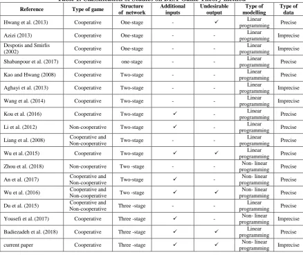
Table 1. Classification of Studies on DEA-Game Theory method

Reference Type of game Structure of network

Additional inputs

Undesirable output

Type of modelling

Type of data

Hwang et al. (2013) Cooperative One-stage -  Linear

programming Precise

Azizi (2013) Cooperative One-stage - - Linear

programming Imprecise Despotis and Smirlis

(2002) Cooperative One-stage - -

Linear

programming Imprecise

Shabanpour et al. (2017) Cooperative one-stage - - Linear

programming Precise

Kao and Hwang (2008) Cooperative Two-stage - - Linear

programming Precise

Aghayi et al. (2013) Cooperative Two-stage - - Linear

Wang et al. (2014) Cooperative Two-stage - - Linear

Kou et al. (2016) Cooperative Two-stage  - Linear

programming Precise

Li et al. (2012) Non-cooperative Two-stage  - Linear

programming Precise

Liang et al. (2008) Cooperative and

Non-cooperative Two-stage - -

Linear

programming Precise

Wu et al.(2015) Cooperative Two-stage   Linear

programming Precise

Zhou et al. (2018) Non-cooperative Two -stage - - Non- linear

programming Precise

An et al. (2017) Cooperative and

Non-cooperative Two-stage  -

Non- linear

programming Precise

Wu et al. (2016) Cooperative and

Non-cooperative Two -stage  

Non- linear

programming Precise

Du et al. (2015) Cooperative and

Non-cooperative Three -stage - -

Linear

programming Precise

Yousefi et al.(2017) Cooperative Three -stage  - Non- linear

Badiezadeh et al. (2018) Cooperative Three -stage   _programmingLinear Precise

current paper Cooperative Three -stage   Non- linear

According to the abovementioned, in major, the researches performed in the network, focused on two stages. But the current research considers the three-stage processes, which in addition to intermediate measures, also has additional inputs and undesirable outputs. In actual fact, DEA signifies a theoretical framework in the way of analyzing efficiency, but its application in the grounds of production planning and inventory control is observed as being extremely low. In this paper we simulate a factory producing dairy products with a production area, three warehouses, two delivery points for goods and we analyze this network in a dynamic condition. Therefore, we are faced with a hybrid system, including a complex internal structure with three stages, six sub-DMUs, and undesirable outputs in the first stage, additional inputs and outputs in the second stage and additional inputs and undesirable outputs in the third stage. Interval data is utilized to evaluate efficiency, in order to make results more realistic. Likewise, in this paper, the cooperative approach is used to evaluate efficiency and a heuristic method is applied to convert nonlinear models to linear models. As a summarization, contributions of this paper are as follows:

 A three-stage network is taken under consideration in respect to the additional desirable and undesirable inputs and outputs

 A hybrid system with a complex internal structure is developed by a DEA approach.

 Interval data is utilized to evaluate efficiency, in order to make results more realistic

(5)

 Implementation of the suggested model on an authentic example. (We simulate a factory in a real world that has a production area and three warehouses for goods and two delivery points for first time .

 The said factory is considered as a dynamic network.

 In this simulation, all costs are considered, including, production costs, setup cost, maintenance costs of the products, warehouse reservation costs, transportation costs, delay penalty costs and the profit obtained from the sale of products.

The remainder of the paper is organized as follows: Section (2) describes the model and introduces the network and modeling from the cooperative perspective for interval data. Section (3) resolves the model and in this section a heuristic approach is used to solve the model. Section (4) describes a case-study, where, a factory is elaborated upon as an example in the factual world and ultimately Section (5) renders the results of the paper.

2. Model description

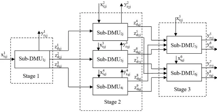
We consider a set of n homogeneous DMUs that are denoted by DMUj (j=1,..., n), and the each DMUj (j=1,…,n) has a three-stage with a complex internal structure, as shown in Fig. 1. We

denote, the inputs to sub-DMU1j, sub-DMU2j, sub-DMU3j, sub-DMU4j, sub-DMU5j and

sub-DMU₆_j by x_i1₁_j (i₁=1,…,I₁), x_i2₂_j (i₂=1,…,I₂), x_i3₃_j (i₃=1,…,I₃), x_i4₄_j (i₄=1,…,I₄), x_i5₅_j (i₅=1,…,I₅) and x_i6₆_j (i₆=1,…,I₆), respectively. We denote, the intermediate measures between stage 1 and 2 by z_d1₁_j (d₁=1,…,D₁), z2_d₂_j (d₂=1,…,D₂) and z_d3₃_j(d₃=1,…,D₃), and between stage 2 and 3 by z_d4₄_j_(d

4=1,…,D4), zd5j

5 ₍_d

5 = 1, … , D5), zd6j

6 ₍_d

6 = 1, … , D6), zd7j

7 ₍_d

7 = 1, … , D7), zd8j 8

(d₈=1,…,D₈) and z_d9₉_j (d₉=1,…,D₉). We denote, the undesirable output of the first stage by y_r1₁_j_(r

1=1,…,R1). The outputs of sub-DMU2j, sub-DMU3j and sub-DMU4j are denoted by y_r2₂_j_(r

2=1,…,R2), yr3j

3 _(r

3=1,…,R3) and yr4j

4 _(r

4=1,…,R4), respectively. Finally, the outputs of sub-DMU₅_j and sub-DMU₆_j are denoted by y_r5₅_j (r₅=1,…,R₅), y_r6₆_j (r₆=1,…,R₆), y_r7₇_j (r₇=1,…,R₇) and y_r8₈_j (r₈=1,…,R₈), respectively where y_r6₆_j and y_r8₈_j are undesirable outputs. We adopt v_i1₁, v_i2₂, v_i3₃, v_i4₄, v_i5₅ and v_i6₆ as the weights of the inputs to sub-DMU1j, sub-DMU2j,

(6)

Figure. 1 The structure of three-stage network system with additional inputs and undesirable outputs

It is mainly for three reasons that researchers are most likely to use input-oriented models for efficiency analysis. Primarily, demand is in a state of growth and the estimation of demand is a complex issue. Secondly, managers have more control over inputs than outputs; and thirdly, this model reflects the initial goals or objectives of policy-makers, in being responsible for responding to the demands of the people and that the units should reduce costs and or limit the use of resources. Thereby, we utilize the input-axis model in this research. In accordance with Korhonen and Luptacik (2004), we signify the undesirable outputs in the models with a negative mark. Therefore, the efficiency of sub-DMU_1o in the first stage can be calculated using the following model (1):

θo1= max

∑D1_d1=1w_d11z_d1o1 + ∑D2_d2=1w_d22z_d2o2 + ∑D3_d3=1w_d33z_d3o3 - ∑ u_r11_y r1o1 R1 r1=1

∑I1_i1=1v_i11x_i1o1

s.t. ∑ wd1

1 D1

d1=1 zd1j1 + ∑d2=1D2 wd22zd2j2 + ∑D3d3=1wd33zd3j3 - ∑R1r1=1ur11yr1j1

∑I1_i1=1v_i11x_i1j1 ≤1, j=1,…,n (1)

ur11,vi1

1_{, w}

d1₁,wd2₂,wd3₃≥ 𝜀; r1=1,…,R1; i1=1,…,I1; d1=1,…,D1; d2=1,…,D2; d3=1,…,D3.

In the second stage we have three sub-DMUs form a parallel structure and the sub-DMUs are independent. The efficiencies of sub-DMU₂_o, sub-DMU₃_o and sub-DMU₄_o are defined, respectively, as follows:

θo2= max

∑D4_d4=1w_d44z_d4o4 + ∑_d5=1D5 w5_d5z_d5o5 + ∑R2_r2=1u_r22y_r2o2

∑I2_i2=1v_i22x_i2o2 + ∑D1_d1=1w_d11 z_d1o1

s.t. ∑ wd4

4 D4

d4=1 zd4j4 + ∑D5d5=1wd55zd5j5 + ∑R2r2=1ur22yr2j2

∑I2_i2=1v_i22x_i2j2+ ∑D1_d1=1w_d11z_d1j1 ≤1, j=1,…,n (2)

ur2₂,vi2

2_{, w}

d1

1 _,w

d4

4 _,w

d5

5 _{≥ 𝜀; r}

2=1,…,R2; i2=1,…,I2; d1=1,…,D1; d4=1,…,D4; d5=1,…,D5.

θo3= max

∑D6_d6=1w_d66z_d6o6 + ∑D7_d7=1w_d77z_d7o7 + ∑ u_r33_y r3o 3 R3 r3=1

(7)

s.t. ∑ wd6

6 D6

ur3₃,vi3₃, wd2

2 _,w

d6

6 _,w

d7

7 _{≥ 𝜀; r}

3=1,…,R3; i3=1,…,I3; d2=1,…,D2; d6=1,…,D6; d7=1,…,D7.

θo4= max

∑D8_d8=1w_d88 z_d8o8 + ∑D9_d9=1w_d99z_d9o9 + ∑ u_r44_y r4o4 R4 r4=1

∑I4_i4=1v_i44x_i4o4 + ∑D3_d3=1w_d33z_d3o3

s.t. ∑ wd8

8 D8

∑I4_i4=1v_i44x_i4j4 + ∑D3_d3=1w3_d3z_d3j3 ≤1, j=1,…,n (4)

ur44,vi4

4_{, w}

d₃

3 _,w

d8₈,wd9₉≥ 𝜀; r3=1,…,R3; i4=1,…,I4; d4=1,…,D4; d8=1,…,D8; d9=1,…,D9.

Kao (2009) used the additive approach for the overall efficiency of a parallel structure where sub-DMUs are independent. We then define the efficiency of the second stage as: θo234=max (w1.θo2+w2.θo3+w3.θo4), where w1, w2 and w3 are weights specified by experts such that, w1 + w2 + w3 = 1. Chen et al. (2009), show that, the relative size of the inputs of a stage expresses the importance of that stage. Hence, based on the fact that our model is input-oriented, we compute the weights determined by the experts from the relative input value of each sub-DMU to implicit the value of inputs in the second stage. Thereby, we define w₁,w₂

andw₃asfollows:

w1=

∑I2_i2=1v_i22x_i2o2 + ∑D1_d1=1w_d11z_d1o1

∑I2_i2=1v_i22x_i2o2 + ∑D1_d1=1w_d11 z_d1o1 + ∑I3_i3=1v_i33x_i3o3 + ∑D2_d2=1w_d22z_d2o2 + ∑_i4=1I4 v4_i4x_i4o4 + ∑D3_d3=1w_d33 z_d3o3 , (5)

w2=

∑I3_i3=1v_i33x_i3o3 + ∑D2_d2=1w_d22z_d2o2

∑I2_i2=1v_i22x_i2o2 + ∑_d1=1D1 w1_d1z_d1o1 + ∑I3_i3=1v_i33x_i3o3 + ∑D2_d2=1w_d22z_d2o2 + ∑I4_i4=1v_i44x_i4o4 + ∑D3_d3=1w_d33 z_d3o3 ,

w3=

∑I4_i4=1v_i44x_i4o4 + ∑D3_d3=1w_d33z_d3o3

∑I2_i2=1v_i22x_i2o2 + ∑_d1=1D1 w1_d1z_d1o1 + ∑I3_i3=1v_i33x_i3o3 + ∑D2_d2=1w_d22z_d2o2 + ∑I4_i4=1v_i44x_i4o4 + ∑D3_d3=1w_d33 z_d3o3

We defined w1, w2 and w3 as the parts of total input resources devoted to the sub-DMU2o, sub-DMU3o and sub-DMU4o, respectively. In order to make the models more convenient, we define I_o234 and O_o234, as inputs and outputs to the second stage, respectively, as follows:

(Io234= ∑iI2₂=1vi2₂xi2₂o+ ∑ wd1

1 D₁

d1=1 zd1o

1 _{+ ∑} _v

i3₃xi3₃o I₃

i₃=1 + ∑ wd2

2 D₂

d2=1 zd2o

2 _{+ ∑} _v

i₄

4_x

i4₄o I₄

i₄=1 + ∑ wd3

3 D₂

d2=1 zd3o

3 _{) and}

(Oo234= ∑dD₄4=1wd4₄z4d₄o+ ∑Dd55=1wd5₅zd5o

5 _{+ ∑} _w

d6₆ D₆

d₆=1 zd6₆o+ ∑Dd₇7=1wd7₇z7d₇o+ ∑Dd₈8=1wd8₈zd8₈o+ ∑dD₉9=1wd9₉zd9₉o

+ ∑Rr22=1ur2₂y2r₂o + ∑ ur33yr33o

R₂

r2=1 + ∑ ur44yr44o

R₄

r4=1 ) (6)

Then, with models (2), (3) and (4) and formulas (5) and (6), the efficiency of the second stage is defined as follows:

θo234=max Oo

234

Io234

s.t. ∑ wd4

4 D4

(8)

∑ wd6

6 D6

∑ wd8

8 D8

∑I4_i4=1v_i44x_i4j4+ ∑D3_d3=1w_d33z_d3j3 ≤1, j=1,…,n

ur22,ur33,ur44,vi2

2_,v

i3₃,vi4₄,w1d₁,wd2₂,wd3₃,wd4₄,wd5₅,wd6₆,wd7₇,wd8₈,wd9₉ ≥ 𝜀;

r2=1, …,R2; r3=1,…,R3; r4=1,…, R4; i2=1,…,I2; i3=1,…,I3; i4=1,…,I4; d1=1,…,D1; d2=1,…,D2;

d3=1,…,D3; d4=1,…,D4; d5=1,…,D5; d6=1,…,D6;d7=1,…,D7; d8=1,…,D8; d9=1,…,D9.

In the model (7) we measured the efficiency of the second stage, based on the efficiency of each DMU in the second stage being less than one. In the third stage we have two sub-DMUs from a parallel structure. In the same way we define the efficiency of the third stage, as we did in the second stage, as follows:

θo56= max Oo

56

I_o56

s.t. ∑ ur5

5 R5

r5=1 yr5j5 - ∑R6r6=1ur66yr6j6

∑I5_i5=1v_i55x_i5j5 + ∑D4_d4=1w_d44 z_d4j4 + ∑D6_d6=1w6_d6z_d6j6 + ∑D8_d8=1w_d88z_d8j8 ≤1, j=1,…,n

∑ ur77

R7

r7=1 yr7j7 - ∑R8r8=1ur88yr8j8

∑I6_i6=1v_i66x_i6j6 + ∑D5_d5=1w5_d5z_d5j5 + ∑D7_d7=1w_d77z_d7j7 + ∑D9_d9=1w_d99z_d9j9 ≤1, j=1,…,n

(8)

u5r5,ur66,u7r7,ur88,vi5

5_,v i₆

6_,w

d4₄,wd5₅,wd6₆,wd7₇,wd8₈,wd9₉ ≥ 𝜀;

r5=1, …,R5; r6=1,…,R6; r7=1,…, R7; r8=1,…,R8; i5=1,…,I5; i6=1,…,I6; d4=1,…,D4; d5=1,…,D5;

d6=1,…,D6;d7=1,…,D7; d8=1,…,D8; d9=1,…,D9.

Model (8) gains the performance of the third step and to alleviate the input and output values of the third stage we have denoted it in formula (9) as follows:

(Io56= ∑ vi55xi55o

I₅

i₅=1 + ∑ vi66xi66o

I6

i6=1 + ∑ wd4

4 D4

d₄=1 zd4o

4 _{+ ∑} _w

d5₅ D₅

d₅=1 zd5₅o+ ∑ wd6

6 D6

d₆=1 zd6o

6 _{+ ∑} _w

d7

7 D7

d₇=1 zd7o

7

+ ∑ wd8

8 D₈

d8=1 zd8o

8 _{+ ∑} _w

d9

9 D₉

d9=1 zd9o

9 _{) and (O}

o

56_{= ∑} _u

r₅ 5 R₅

r5=1 yr5o

5 _{+ ∑} _u

r₇ 7 R₇

r7=1 yr7o

7 _{- ∑} _u

r₆ 6 R₆

r6=1 yr6o

6 _{- ∑} _u

r₈ 8 R₈

r8=1 yr8o

8 ₎

(9)

θooverall=max

∑D1_d1=1w_d11z_d1o1 + ∑D2_d2=1w_d22z_d2o2 + ∑D3_d3=1w_d33z_d3o3 - ∑R1_r1=1u_r11y_r1o1

∑I1_i1=1v_i11x_i1o1 .

O_o234 I_o234.

O_o56 I_o56

s.t. ∑ wd1

1 D1

d1=1 zd1j1 + ∑d2=1D2 w2d2zd2j2 + ∑D3d3=1wd33zd3j3 - ∑R1r1=1ur11yr1j1

∑I1_i1=1v_i11x_i1j1 ≤1, j=1,…,n

∑ wd4

4 D4

∑I2_i2=1v_i22x_i2j2 + ∑D1_d1=1w_d11 z_d1j1 ≤1, j=1,…,n

∑ wd6

6 D6

∑I3_i3=1v_i33x_i3j3 + ∑D2_d2=1w2_d2z_d2j2 ≤1, j=1,…,n (10)

∑ wd8

8 D8

∑I4_i4=1v_i44x_i4j4 + ∑D3_d3=1w_d33z_d3j3 ≤1, j=1,…,n

∑ ur55

R5

r5=1 yr5j5 - ∑R6r6=1ur66yr6j6

∑R7r7=1ur77y7r7j- ∑R8r8=1ur88yr8j8

ur1₁,ur2₂,ur3₃,ur4₄,ur5₅,ur6₆,u7r₇,ur8₈,vi1

1_,_v i2

2_,_v i3

3_,_v i4

4_,_v i5

5_,v i6

6_,_w

d1

1 _,_w

d2

2 _,_w

d3

3 _,_w

d4 4 _,w d5 5 _,w d6 6 _,w d7 7 _,w d8 8 _,w d9

9 _{≥ ε;}

r1=1, …,R1; r2=1,…,R2; r3=1,…, R3; r4=1, …,R4; r5=1,…,R5; r6=1,…, R6; r7=1, …,R7; r8=1,…,R8;

i1=1,…,I1; i2=1,…,I2; i3=1,…,I3; i4=1,…,I4; i5=1,…,I5; i6=1,…,I6; d1=1,…,D1; d2=1,…,D2; d3=1,…,D3;

d4=1,…,D4; d5=1,…,D5; d6=1,…,D6;d7=1,…,D7; d8=1,…,D8; d9=1,…,D9.

In model (10) we measure the overall efficiency based on the efficiencies of the all sub-DMUs being less than one.

2.1. Interval DEA models

In view of not evading the entire subject, it shall be assumed that some of the data in model (10) due to being unreliable and are incapable of being accurately determined and we only know that they are within their upper and lower bounds. Despotis and Smirlis (2002) have calculated the efficiency of DMUs in the presence of intervals and have proposed models for the upper and lower bound efficiencies. Therefore, by developing the task of Despotis and Smirlis we shall modify model (10), with the assumption that the variables are bounded in the presence of undesirable outputs as in the figure below:

θooverall(U)=max

∑D1_d1=1w_d11z_d1o1U+ ∑D2_d2=1w_d22 z_d2o2U+ ∑D3_d3=1w_d33z_d3o3U- ∑R1_r1=1u_r11y_r1o1L

∑I1_i1=1v_i11x_i1o1L .

O_o234U

Io234L.

O_o56U

Io56L (11)

s.t. ∑Dd11=1wd1₁zd1j

1L_{+ ∑} _w

d2₂ D₂

d2=1 zd2j

2L_{+ ∑} _w

d₃ 3 D₃

d3=1 zd3j

3L_{- ∑} _u

r1

1_y

r₁j 1U R₁

r₁=1 - ∑iI₁1=1vi1₁xi1U₁j ≤ 0, ∀j≠o

∑ wd4

4 D₄

d4=1 zd4j

4L_{+ ∑} _w

d5

5 D₅

d₅=1 zd5j

5L_{+ ∑} _u

r₂

2_y

r2L₂j R₂

r2=1 - ∑ vi2

2_x

i₂j 2U I₂

i2=1 - ∑ wd1

1 D₁

d1=1 zd1j

1U_{≤ 0, ∀j≠o}

∑ wd6

6 D₆

d6=1 zd6j

6L_{+ ∑} _w

d7

7 D₇

d7=1 zd7j

7L_{+ ∑} _u

r₃

3_y

r3L₃j R₃

r3=1 - ∑ vi3

3_x

i₃j 3U I₃

i3=1 - ∑ wd2

2 D₂

d2=1 zd2j

2U_{≤ 0, ∀j≠o}

∑ wd8

8 D₈

d8=1 zd8j

8L_{+ ∑} _w

d9

9 D₉

d9=1 zd9j

9L_{+ ∑} _u

r₄

4_y

r4L₄j R₄

r4=1 - ∑ vi4

4_x

i₄j 4U I₄

i4=1 - ∑ wd3

3 D₃

d3=1 zd3j

3U_{≤ 0, ∀j≠o}

∑ ur55

R₅

r₅=1 yr5L₅j- ∑ ur66

R6

r₆=1 yr6U6j- ∑ vi5

5_x

i₅j 5U I₅

i₅=1 - ∑Dd₄4=1w4d₄zd4U₄j- ∑Dd₆6=1wd6₆zd6U₆j- ∑Dd₈8=1wd8₈zd8U₈j≤ 0, ∀j≠o

(10)

∑Rr77=1ur7₇yr7j

7L_{- ∑} _u

r₈ 8 R₈

r8=1 yr8j

8U_{- ∑} _v

i₆

6_x

i₆j 6U I₆

i6=1 - ∑ wd5

5 D₅

d₅=1 zd5j

5U_{- ∑} _w

d7

7 D₇

d7=1 zd7j

7U_{- ∑} _w

d9

9 D₉

d9=1 zd9j

9U_{≤ 0, ∀j≠o}

∑Dd₁1=1wd1₁zd1U₁o+ ∑dD₂2=1w2d₂zd2U₂o+ ∑dD₃3=1w3d₃zd3U₃o- ∑rR11=1ur1₁yr1L₁o- ∑ vi11xi1L1o

I1

i1=1 ≤ 0

∑Dd₄4=1w4d₄zd4U₄o+ ∑dD₅5=1w5d₅z5Ud₅o+ ∑ ur22yr2U2o

R2

r₂=1 - ∑ vi22xi2L2o

I2

i₂=1 - ∑Dd₁1=1wd1₁zd1L₁o ≤ 0

∑Dd₆6=1wd6₆zd6U₆o+ ∑dD₇7=1wd7₇zd7U₇o+ ∑ ur33yr3U3o

R₃

r₃=1 - ∑Ii₃3=1v3i₃xi3L₃o- ∑dD₂2=1wd2₂zd2L₂o ≤ 0

∑Dd₈8=1w8d₈zd8U₈o+ ∑dD₉9=1w9d₉z9Ud₉o+ ∑ ur44yr4U4o

R₄

r₄=1 - ∑Ii₄4=1vi4₄xi4L₄o- ∑dD₃3=1wd3₃zd3L₃o ≤ 0

∑Rr55=1ur5₅yr5U5o- ∑ ur66

R₆

r6=1 yr6L6o- ∑ vi5

5_x

i₅o 5L I₅

i5=1 - ∑ wd4

4 D₄

d4=1 zd4o

4L_{- ∑} _w

d6

6 D₆

d6=1 zd6o

6L _{- ∑} _w

d8

8 D₈

d8=1 zd8o

8L _{≤ 0}

∑Rr77=1ur7₇yr7U7o- ∑ ur88

R8

r8=1 yr8L8o- ∑ vi66xi6L6o

I6

i6=1 - ∑ wd5

5 D₅

d₅=1 zd5L₅o- ∑ wd7

7 D7

d7=1 zd7o

7L _{- ∑} _w

d9

9 D9

d9=1 zd9o

9L _{≤ 0}

u1r1,ur22,u3r3,ur44,ur55,ur66,u7r7,ur88,vi1

1_,_v

i2₂,vi3₃,vi4₄,vi5₅,vi6₆,wd1₁,w2d₂,wd3₃,wd4₄,wd5₅,wd6₆,wd7₇,wd8₈,wd9₉ ≥ ε;

d4=1,…,D4; d5=1,…,D5; d6=1,…,D6;d7=1,…,D7; d8=1,…,D8; d9=1,…,D9.

θooverall(L)=max

∑D1_d1=1w_d11z_d1o1L + ∑D2_d2=1w_d22z_d2o2L + ∑D3_d3=1w_d33 z_d3o3L- ∑R1_r1=1u_r11y_r1o1U

∑I1_i1=1v_i11x_i1o1U .

O_o234L

Io234U.

O_o56L

Io56U (12)

s.t. ∑ wd1

1 D₁

d1=1 zd1j

1U_{+ ∑} _w

d2

2 D₂

d2=1 zd2j

2U_{+ ∑} _w

d3

3 D₃

d3=1 zd3j

3U_{- ∑} _u

r₁

1_y

r₁j 1L R₁

r₁=1 - ∑iI1₁=1vi1₁xi1L₁j ≤ 0, ∀j≠o

∑ wd4

4 D₄

d4=1 zd4j

4U_{+ ∑} _w

d5

5 D₅

d₅=1 zd5j

5U_{+ ∑} _u

r₂

2_y

r2U₂j R₂

r₂=1 - ∑iI₂2=1v2i₂xi2L₂j- ∑ wd1

1 D₁

d1=1 zd1j

1L_{≤ 0, ∀j≠o}

∑ wd6

6 D6

d₆=1 zd6j

6U_{+ ∑} _w

d7

7 D7

d₇=1 zd7j

7U_{+ ∑} _u

r₃

3_y

r3U3j

R3

r3=1 - ∑ vi33xi3L3j

I3

i3=1 - ∑ wd2

2 D2

d₂=1 zd2j

2L_{≤ 0, ∀j≠o}

∑ wd8

8 D8

d₈=1 zd8j

8U_{+ ∑} _w

d9

9 D9

d₉=1 zd9j

9U_{+ ∑} _u

r₄

4_y

r4U4j

R4

r4=1 - ∑ vi44xi4L4j

I4

i4=1 - ∑ wd3

3 D3

d₃=1 zd3j

3L_{≤ 0, ∀j≠o}

∑ ur55

R5

r₅=1 yr5U₅j- ∑ ur66

R6

r₆=1 yr6L6j- ∑ vi5

5_x

i₅j 5L I5

i₅=1 - ∑Dd₄4=1w4d₄zd4L₄j- ∑Dd₆6=1w6d₆zd6L₆j- ∑Dd₈8=1wd8₈zd8L₈j≤ 0, ∀j≠o

∑ ur77

R₇

r₇=1 yr7U₇j- ∑ ur88

R₈

r₈=1 yr8L₈j- ∑iI₆6=1vi6₆x6Li₆j- ∑dD55=1w5d₅zd5j

5L_{- ∑} _w

d₇ 7 D₇

d7=1 zd7j

7L_{- ∑} _w

d₉ 9 D₉

d9=1 zd9j

9L_{≤ 0, ∀j≠o}

∑ wd1

1 D₁

d1=1 zd1o

1L_{+ ∑} _w

d2

2 D₂

d2=1 zd2o

2L _{+ ∑} _w

d3

3 D₃

d3=1 zd3o

3L_{- ∑} _u

r₁

1_y

r₁o 1U R₁

r1=1 - ∑ vi1

1_x

i₁o 1U I₁

i1=1 ≤ 0

∑ wd4

4 D₄

d4=1 zd4o

4L _{+ ∑} _w

d₅ 5 D₅

d₅=1 zd5L₅o+ ∑Rr22=1u2r₂y2Lr₂o- ∑ vi2

2_x

i₂o 2U I₂

i2=1 - ∑ wd1

1 D₁

d1=1 zd1o

1U_{≤ 0}

∑Dd₆6=1wd6₆zd6L₆o+ ∑dD₇7=1wd7₇zd7L₇o+ ∑ ur33yr3L3o

R3

r₃=1 - ∑ vi33xi3U3o

I3

i₃=1 - ∑Dd₂2=1wd2₂zd2U₂o ≤ 0

∑Dd₈8=1w8d₈zd8L₈o+ ∑dD₉9=1w9d₉z9Ld₉o+ ∑ ur44yr4L4o

R4

r₄=1 - ∑ vi44xi4U4o

I4

i₄=1 - ∑Dd₃3=1wd3₃zd3U₃o ≤ 0

∑Rr55=1ur5₅yr5o

5L_{- ∑} _u

r₆ 6 R₆

r₆=1 yr6U₆o- ∑Ii55=1vi5₅x5Ui₅o- ∑ wd4

4 D₄

d4=1 zd4o

4U_{- ∑} _w

d6

6 D₆

d6=1 zd6o

6U_{- ∑} _w

d8

8 D₈

d8=1 zd8o

8U_{≤ 0}

∑Rr77=1ur7₇yr7L7o- ∑ ur88

R₈

r8=1 yr8U8o- ∑ vi6

6_x

i₆o 6U I₆

i6=1 - ∑ wd5

5 D₅

d₅=1 zd5o

5U_{- ∑} _w

d7

7 D₇

d7=1 zd7o

7U_{- ∑} _w

d9

9 D₉

d9=1 zd9o

9U_{≤ 0}

u1r1,ur22,u3r3,ur44,ur55,ur66,u7r7,ur88,vi1

1_,_v

i2₂,vi3₃,vi4₄,vi5₅,vi6₆,wd1₁,w2d₂,wd3₃,wd4₄,wd5₅,wd6₆,wd7₇,wd8₈,wd9₉ ≥ ε;

(11)

Model (11) measures the efficiency under the most desirable conditions which is known as the ‘upper bound efficiency’; whereas, model (12) measures the efficiency under the most undesirable conditions and is known as the ‘lower bound efficiency’. It should be noted that the undesirable output have similar characteristics to that of the inputs, thereby, their boundaries are also considered alike the inputs. Models (11) and (12) are nonlinear and are obtained by multiplying their objective function. In the third section of this paper, an innovative approach is used to solve them. Let us assume that the models (11) and (12) are resolved, the interval efficiency of the network illustrated in Fig. 1 for DMU0 in the [θ_ooverall(L),θ_ooverall(U)] manner. In order to compare the interval efficiency and the ranking of DMUs, a minimax regret-based approach was proposed by Wang et al. (2005) and we shall use this approach to rank the units. Wang et al. has also stated that, the interval efficiency with the slightest waste of efficiency would be the optimal efficiency interval. They defined the criteria for the minimax regret-based approach for the efficiency interval as = 𝐴_𝑖[𝑎_𝑖𝐿, 𝑎_𝑖𝑈], (𝑖 = 1 … 𝑛) which has been described in formula (13) as below:

𝑅(𝐴𝑖) = 𝑚𝑎𝑥 (max_𝑗≠𝑖(𝑎𝑗𝑈) − 𝑎𝑖𝐿, 0) ,

(𝑖 = 1 … 𝑛) (13)

On the basis of which, we first calculate the maximum loss for each interval and consider the minimum loss, as the most desirable or favorable interval. In the next stage we eliminate the desirable interval and repeatedly, in the same manner, from the remaining n-1 select the optimal interval and this is iteratively performed until only one interval efficiency remains; and the lowest position is assigned to this.

3. Model solution

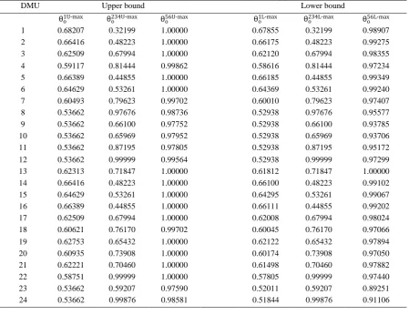
Models (11) and (12) cannot be turned into linear models because of the additional outputs in the first stage in relative to sub-DMU_1o, the additional inputs and outputs in the second stage related to sub-DMU_2o, sub-DMU_3o and sub-DMU_4o and the additional inputs in the third stage in relevance to sub-DMU_5o and sub-DMU_6o respectively. Thus, we propose the heuristic approach given hereunder, for solving models (11) and (12). This approach shall be founded on model (11). We are aware that the objective function of model (11) is the product of the efficiency of the three phases i.e. θooverall(U)=max θ1Uo . θo234U . θo56U. First, we measure the maximum efficiency of each stage provided that the efficiency of each sub-DMU in stage 1, stag 2 and stage 3 is less than one. Therefore, we define θ_o1U-max, θ_o234U-max and θ_o56U-max maximum efficiencies for stage 1, stage 2 and stage 3, respectively as follows:

θo1U-max=max { θo

1U_{| θ}

j

1L_{≤ 1, θ}

j

2L_{≤ 1, θ}

j

3L_{≤ 1, θ}

j

4L_{≤ 1, θ}

j

5L_{≤ 1, θ}

j

6L_{≤ 1, ∀j≠o,}

θo1U ≤ 1, θo2U ≤ 1, θo3U ≤ 1,θo4U ≤ 1, θo5U ≤ 1, θo6U ≤ 1

} (14)

θo234U-max=max {θo

234U_{| θ}

j

1L_{≤ 1, θ}

j

2L_{≤ 1, θ}

j

3L_{≤ 1, θ}

j

4L_{≤ 1, θ}

j

5L_{≤ 1, θ}

j

6L_{≤ 1, ∀j≠o,}

θo1U ≤ 1, θo2U ≤ 1, θo3U ≤ 1,θo4U ≤ 1, θo5U ≤ 1, θo6U ≤ 1

}

θo56U-max=max {θo

56U_{| θ}

j

1L_{≤ 1, θ}

j

2L_{≤ 1, θ}

j

3L_{≤ 1, θ}

j

4L_{≤ 1, θ}

j

5L_{≤ 1, θ}

j

6L_{≤ 1, ∀j≠o,}

θo1U ≤ 1, θo2U ≤ 1, θo3U ≤ 1, θo4U ≤ 1, θo5U ≤ 1, θo6U ≤ 1

}

(12)

respectively. The objective function of model (11) is θ_o1U . θ_o234U . θ_o56U and an upper bound can be obtained for each one. We suggest a heuristic method to solve model (11) by using two models as follows:

Step 1: In the first model let us consider two stages for example θ_o1U and θ_o234U as two variables that change between intervals [0, θo1U-max ] and [0, θo234U-max ], respectively. Then the maximal efficiency of model (11) and the maximal and minimal efficiency of θ_o1U and θ_o234U are obtained, provided that the efficiency of model (11) is fixed or constant.

Step 2: In the second model consider another two stages for example θ_o234U and θ_o56U as two variables and as in the first model, it obtains the maximal efficiency of model (11) and the maximal and the minimal efficiency of θ_o234U and θ_o56U .

By using two abovementioned steps we obtain the maximal efficiency of the model (11) and the maximal and minimal efficiency of one stage twice, that is, with a very agreeable approximation, which is equivalent. We perform the two abovementioned steps three times and consider all the modes. In the continuation of this paper, we shall consider one of the modes. First, we convert model (11) to model (15) and use a heuristic method to solve it as follows:

θooverall(U)=max

{

θo1U. θo234U. θo56U

| |

θj1L ≤ 1, θj2L ≤ 1, θj3L ≤ 1, θj4L ≤ 1, θj5L ≤ 1, θj6L ≤ 1, ∀j≠o,

θo1U= Oo

1U

I_o1L, θo

234U₌Oo234U

I_o234L, θo

1U _{∈[0, θ}

o 1U-max _],

θo234U ∈[0, θo234U-max ] }

(15)

In the models (15) all the variables are non-negative. It should be noted that in the model (15), we consider θ_o1U ,θo234Uas two variables in the objective function and the two constraints

which specify these two variables, together with the interval modifications are supplemented to the model by us. In model (1), we have described the efficiency of the first stage and in model (15) have briefly demonstrated byoutputs to inputs. In model (15) let us consider stage 1 and 2 as two variables θ_o1U and θ_o234U that change between intervals [0, θ_o1-max ] and [0,

θ_o234-max _]_{, respectively. We should fix}_θ

o

1U_{and θ} o

234U_{until model (15) becomes a linear}

programing model and we can solve it. For this purpose, we define θ_o1U and θ_o234U as follows:

θo1U = θo1U-max - k1∆ε, k1=0,1,…, [θo

1U-max

∆ε ] +1 (16)

θo234U = θo234U-max - k2∆ε, k2=0,1,…, [θo

234U-max

∆ε ] +1

In the model (16), ∆𝜀 is a step size and we consider ∆ε =0.01. With the Charnes–Cooper (1962) converted models, model (15) can be turned into a linear model as follows:

Let T= 1

∑I5_i5=1v_i55x_i5o5L+∑I6_i6=1v6_i6x_i6o6L+∑D4_d4=1w4_d4z_d4o4L +∑D5_d5=1w5_d5z_d5o5L+∑D6_d6=1w6_d6z_d6o6L+∑_d7=1D7 w_d77z_d7o7L +∑D8_d8=1w8_d8z_d8o8L +∑D9_d9=1w9_d9z_d9o9L , thus:

θooverall(U) = max θo1U. θo234U. (∑rR₅5=1ur5₅y5Ur₅o+ ∑ ur77

R₇

r₇=1 yr7U7o- ∑ ur66

R₆

r₆=1 yr6L6o- ∑ ur88

R₈

r₈=1 yr8L8o )

(17)

s.t. ∑dD₁1=1wd1₁zd1L₁j+ ∑Dd₂2=1wd2₂z2Ld₂j+ ∑Dd₃3=1wd3₃z3Ld₃j- ∑ ur11yr1U1j

R₁

r₁=1 - ∑ vi11xi1U1j

I₁

i₁=1 ≤ 0, ∀j≠o

∑Dd44=1wd4₄zd4j

4L_{+ ∑} _w

d₅ 5 D₅

d5=1 zd5j

5L_{+ ∑} _u

r2

2_y

r2L₂j R₂

r₂=1 - ∑Ii2₂=1vi2₂xi2U₂j- ∑dD11=1wd1₁zd1j

1U_{≤ 0, ∀j≠o}

∑ wd6

6 D6

d6=1 zd6j

6L_{+ ∑} _w

d7

7 D7

d7=1 zd7j

7L_{+ ∑} _u

r₃

3_y

r₃j 3L R3

r3=1 - ∑ vi3

3_x

i3U₃j I3

i3=1 - ∑ wd2

2 D2

d2=1 zd2j

2U_{≤ 0, ∀j≠o}

∑ wd8

8 D8

d8=1 zd8j

8L_{+ ∑} _w

d9

9 D9

d9=1 zd9j

9L_{+ ∑} _u

r₄

4_y

r4j

4L R4

r4=1 - ∑ vi44xi4U4j

I4

i4=1 - ∑ wd3

3 D3

d3=1 zd3j

(13)

∑Rr₅5=1ur5₅yr5L₅j- ∑Rr66=1ur6₆yr6j

6U_{- ∑} _v

i5₅xi5U₅j I₅

i₅=1 - ∑ wd4

4 D₄

d4=1 zd4j

4U_{- ∑} _w

d6

6 D₆

d6=1 zd6j

6U_{- ∑} _w

d8

8 D₈

d8=1 zd8j

8U_{≤ 0, ∀j≠o}

∑Rr77=1ur7₇yr7L7j- ∑ ur88

R8

r8=1 yr8U8j- ∑ vi66xi6U6j

I6

i6=1 - ∑ wd5

5 D₅

d₅=1 zd5U₅j- ∑dD₇7=1wd7₇zd7U₇j- ∑Dd₉9=1wd9₉zd9U₉j ≤0 ∀j≠o

∑dD₁1=1wd1₁z1Ud₁o+ ∑Dd₂2=1wd2₂z2Ud₂o+ ∑Dd₃3=1wd3₃z3Ud₃o- ∑ ur11yr1L1o

R₁

r₁=1 - ∑iI1₁=1vi1₁xi1L₁o ≤ 0

∑ wd4

4 D₄

d4=1 zd4o

4U_{+ ∑} _w

d5

5 D₅

d5=1 zd5o

5U_{+ ∑} _u

r₂

2_y

r2U₂o R₂

r₂=1 - ∑iI2₂=1v2i₂xi2L₂o- ∑ wd1

1 D₁

d1=1 zd1o

1L _{≤ 0}

∑ wd6

6 D₆

d6=1 zd6o

6U_{+ ∑} _w

d7

7 D₇

d7=1 zd7o

7U_{+ ∑} _u

r₃

3_y

r₃o 3U R₃

r3=1 - ∑ vi3

3_x

i₃o 3L I₃

i3=1 - ∑ wd2

2 D₂

d2=1 zd2o

2L_{≤ 0}

∑ wd8

8 D₈

d8=1 zd8o

8U_{+ ∑} _w

d9

9 D₉

d9=1 zd9o

9U_{+ ∑} _u

r₄

4_y

r4U₄o R₄

r4=1 - ∑ vi4

4_x

i₄o 4L I₄

i4=1 - ∑ wd3

3 D₃

d3=1 zd3o

3L _{≤ 0}

∑ ur55

R₅

r₅=1 yr5U5o- ∑ ur66

R6

r6=1 yr6L6o- ∑ vi55xi5L5o

I₅

i₅=1 - ∑Dd₄4=1wd4₄zd4L₄o- ∑Dd₆6=1wd6₆zd6L₆o- ∑Dd₈8=1wd8₈zd8L₈o≤ 0

∑ ur77

R7

r₇=1 yr7U7o- ∑ ur88

R8

r₈=1 yr8L8o- ∑ vi66xi6L6o

I6

i₆=1 - ∑dD55=1wd5₅zd5o

5L _{- ∑} _w

d7₇ D7

d₇=1 zd7L₇o- ∑dD₉9=1w9d₉zd9L₉o ≤ 0

∑Ii₅5=1vi5₅x5Li₅o+ ∑Ii66=1vi6₆x6Li₆o+ ∑ wd4

4 D₄

d4=1 zd4o

4L _{+ ∑} _w

d₅ 5 D₅

d₅=1 zd5L₅o+ ∑ wd6

6 D₆

d6=1 zd6o

6L _{+ ∑} _w

d7

7 D₇

d7=1 zd7o

7L

+ ∑Dd₈8=1wd8₈zd8L₈o+ ∑dD₉9=1wd9₉zd9L₉o =1

Oo1U= Io1L. θo1U

Oo234U= Io234L. θo234U

θo1U ∈[0, θo1U-max ]

θo234U ∈[0, θo234U-max ]

u1r₁,ur2₂,ur3₃,u4r₄,ur5₅,ur6₆,ur7₇,u8r₈,vi11,vi22,vi33,vi44,vi55,vi66,wd1

1 _,_w

d2₂,wd3₃,wd4₄,wd5₅,wd6₆,wd7₇,wd8₈,wd9₉ ≥ ε;

d4=1,…,D4; d5=1,…,D5; d6=1,…,D6;d7=1,…,D7; d8=1,…,D8; d9=1,…,D9.

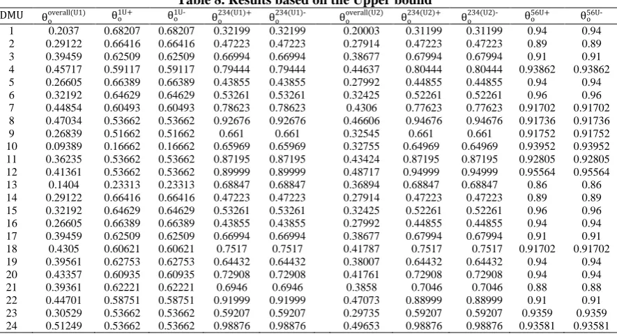
In model (17) we increase k1 and k2 from zero to the upper bound of each one of them independently and solve each linear model with both k1 and k2 and show the value of the objective function with θ_ooverall(U1)(k₁, k₂). In comparing all the values of the objective function in model (17), we define the maximal overall efficiency as θ_ooverall(U1)=max θ_ooverall(U1)(k1, k2). The maximal and minimal efficiencies of the first stage are defined as θo1U+=max θo1U(k1) where, k1=min (k1 |θooverall(U1)(k1, k2) = θooverall(U1)) and θo1U-=min θo1U(k1) where,

k₁=max (k₁ |θ_ooverall(U1)(k₁, k₂) = θ_ooverall(U1)), respectively. Similarly, the maximal and

minimal efficiencies of the second stage are defined as θ_o234(U1)+=max θ_o234U(k₂) where, k₂=min (k₂ |θ_ooverall(U1)(k₁, k₂) = θoverall(U1)_o ) and θ_o234(U1)-=min θ_o234U(k₂) where, k₂=max (k₂ |θ_ooverall(U1)(k₁, k₂) = θ_ooverall(U1)), respectively. If θ_o1U+=θ_o1U- and

θ_o234(U1)+=θ_o234(U1)- we obtain a unique efficiency for the third stage as

follows: θ_o56U= θo overall(U1)

θo1U . θo234(U1)

. Or else, for measuring the maximal and minimal efficiency of the

(14)

θooverall(U)=max

{

θo1U. θo234U. θo56U

| |

θj1L ≤ 1, θj2L ≤ 1, θj3L ≤ 1, θj4L ≤ 1, θj5L ≤ 1, θj6L ≤ 1, ∀j≠o,

θo234= Oo

234

Io234, θo

56₌Oo56

Io56,

θo234U ∈[0, θo234U-max ], θo56U ∈[0, θo56U-max ], j=1,…,n }

(18)

In model (18) we consider stages 2 and 3 as two variables θ_o234U and θ_o56U that change between intervals [0, θ_o234U-max ] and [0, θ_o56U-max ], respectively. We define θ_o234U and θ_o56U as follows:

θo234U = θo234U-max - k2∆ε, k2=0,1,…, [θo

234U-max

∆ε ] +1

(19)

θo56U = θo56U-max - k3∆ε, k3=0,1,…, [θo

56U-max

∆ε ] +1

In model (19) we consider ∆𝜀 =0.01. With the Charnes–Cooper (1962) converted model (18) can be turned into a linear model as follows:

Let T= 1

∑ v_i11_x

i1o 1L I1 i1=1

, thus:

θooverall(U) = max θo234U . θo56U. ( ∑ wd1

1 D₁

d1=1 zd1o

1U_{+ ∑} _w

d2

2 D₂

d2=1 zd2o

2U_{+ ∑} _w

d3

3 D₃

d3=1 zd3o

3U_{- ∑} _u

r₁

1_y

r1L₁o R₁

r₁=1 ) (20)

s.t. ∑dD₁1=1wd1₁zd1L₁j+ ∑Dd₂2=1wd2₂z2Ld₂j+ ∑Dd₃3=1wd3₃z3Ld₃j- ∑ ur11yr1j

1U R₁

r₁=1 - ∑iI₁1=1vi1₁xi1U₁j ≤ 0, ∀j≠o

∑ wd4

4 D₄

d4=1 zd4j

4L_{+ ∑} _w

d5

5 D₅

d₅=1 zd5j

5L_{+ ∑} _u

r₂

2_y

r2L₂j R₂

r₂=1 - ∑iI2₂=1vi2₂xi2U₂j- ∑ wd1

1 D₁

d1=1 zd1j

1U_{≤ 0, ∀j≠o}

∑ wd6

6 D6

d₆=1 zd6j

6L_{+ ∑} _w

d7

7 D7

d₇=1 zd7j

7L_{+ ∑} _u

r₃

3_y

r3j

3L R3

r3=1 - ∑ vi33xi3U3j

I3

i3=1 - ∑ wd2

2 D2

d₂=1 zd2j

2U_{≤ 0, ∀j≠o}

∑ wd8

8 D8

d₈=1 zd8j

8L_{+ ∑} _w

d9

9 D9

d₉=1 zd9j

9L_{+ ∑} _u

r₄

4_y

r4j

4L R4

r4=1 - ∑ vi44xi4U4j

I4

i4=1 - ∑ wd3

3 D3

d₃=1 zd3j

3U_{≤ 0, ∀j≠o}

∑ ur55

R₅

r₅=1 yr5L5j- ∑ ur66

R6

r₆=1 yr6U6j- ∑ vi55xi5U5j

I₅

i₅=1 - ∑Dd₄4=1wd4₄zd4U₄j- ∑Dd₆6=1wd6₆zd6U₆j- ∑Dd₈8=1wd8₈zd8U₈j≤ 0, ∀j≠o

∑ ur77

R7

r₇=1 yr7L7j- ∑ ur88

R8

r₈=1 yr8U8j- ∑ vi66xi6U6j

I6

i₆=1 - ∑dD55=1wd5₅zd5j

5U_{- ∑} _w

d7₇ D7

d₇=1 zd7U₇j- ∑Dd₉9=1wd9₉zd9U₉j ≤ 0, ∀j≠o

∑ wd1

1 D₁

d1=1 zd1o

1U_{+ ∑} _w

d2

2 D₂

d2=1 zd2o

2U_{+ ∑} _w

d3

3 D₃

d3=1 zd3o

3U_{- ∑} _u

r₁

1_y

r1L₁o R₁

r1=1 - ∑ vi1

1_x

i1L₁o I₁

i1=1 ≤ 0

∑ wd4

4 D4

d4=1 zd4o

4U_{+ ∑} _w

d5₅ D₅

d₅=1 zd5U₅o+ ∑Rr22=1u2r₂yr2U₂o- ∑ vi2

2_x

i₂o 2L I2

i2=1 - ∑ wd1

1 D1

d1=1 zd1o

1L _{≤ 0}

∑Dd₆6=1wd6₆zd6U₆o+ ∑dD₇7=1w7d₇z7Ud₇o+ ∑ ur33yr3U3o

R3

r₃=1 - ∑ vi33xi3L3o

I3

i₃=1 - ∑Dd₂2=1w2d₂zd2L₂o ≤ 0

∑Dd₈8=1wd8₈zd8U₈o+ ∑dD₉9=1wd9₉zd9U₉o+ ∑ ur44yr4U4o

R4

r₄=1 - ∑ vi44xi4L4o

I4

i₄=1 - ∑Dd₃3=1wd3₃zd3L₃o ≤ 0

∑Rr55=1ur5₅yr5o

5U_{- ∑} _u

r6

6 R₆

r₆=1 yr6L6o- ∑ vi5

5_x

i₅o 5L I5

i5=1 - ∑ wd4

4 D₄

d4=1 zd4o

4L _{- ∑} _w

d6₆ D₆

d6=1 zd6o

6L _{- ∑} _w

d₈ 8 D₈

d8=1 zd8o

8L_{≤ 0}

∑Rr77=1ur7₇yr7o

7U_{- ∑} _u

r₈ 8 R₈

r8=1 yr8o

8L_{- ∑} _v

i6₆xi6L₆o I₆

i6=1 - ∑ wd5

5 D₅

d₅=1 zd5o

5L _{- ∑} _w

d7

7 D₇

d7=1 zd7o

7L _{- ∑} _w

d9

9 D₉

d9=1 zd9o

9L_{≤ 0}

∑ vi11xi1L1o

I1

i1=1 =1

Oo234U= θo234U.Io234L

Oo56U= θo56U. Io56L

θo234U ∈[0, θo234U-max ]

(15)

u1r₁,ur2₂,ur3₃,u4r₄,ur5₅,ur6₆,ur7₇,u8r₈,vi11,vi22,vi33,vi44,vi55,vi66,wd1

1_,_w

d2₂,wd3₃,wd4₄,wd5₅,wd6₆,wd7₇,wd8₈,wd9₉ ≥ ε;

d4=1,…,D4; d5=1,…,D5; d6=1,…,D6;d7=1,…,D7; d8=1,…,D8; d9=1,…,D9.

We increase k2 and k3 from zero to the upper bound of each one of them, independently and solve each linear model with both k2 and k3 and show the value of the objective function with

θ_ooverall(U2)(k₂, k₃). In comparing all the values of the objective function in the model (20), we

define the maximal overall efficiency as θ_ooverall(U2)=max θ_ooverall(U2)(k2, k3). The maximal and minimal efficiencies of the second stage are defined as θ_o234(U2)+=max θ_o234(k₂) where, k₂=min (k₂ |θ_ooverall(U2)(k₂, k₃) = θoverall(U2)_o ) and θ_o234(U2)- = min θ_o234(k₂) where, k2=max (k2 |θooverall(U2)(k2, k3) = θooverall(U2)), respectively. Similarly, the maximal and minimal efficiencies of the third stage are defined as θ_o56U+=max θ_o56U(k₃) where, k₃=min

(k₃ |θ_ooverall(U2)(k₂, k₃) = θ_ooverall(U2)) and θ_o56U-_{=min θ}

o

56U_(k

3), where, k3=max (k3

|θ_ooverall(U2)(k2, k3) = θooverall(U2)), respectively. Note, that the efficiency of structure as shown

in Fig. 1. is unique and with a very agreeable approximation we obtain:

θ_ooverall(U)=θ_ooverall(U1)= θ_ooverall(U2); θ_o234U+_=θ

o

234(U1)+_{= θ}

o

234(U2)+_;

θo234L-=θo234(L1)-= θo234(L2)-. We obtain the maximal efficiency of the system θooverall(U) and the

maximal and minimal efficiencies for the stages θ_o1U+, θ_o1U−, θ234U+_o , θ_o234U−, θ_o56U+ and θ_o56U− respectively. Note, that if (θ_o1U+=θ_o1U− and θ_o234U+=θ_o234U−) or (θ_o1U+=θ_o1U− and θo56U+=θo56U−) or (θo234U+=θo234U− and θo56𝑈+=θo56U−) then we have a unique efficiency for each stage based on θ_ooverall(U)= θ_o1U. θ_o234U. θ_o56U. We tested our proposed approach in three modes and each time denoted two different stages as variables. Given the fact that, the efficiency of a network is unique, hence, the results of these three methods were approximately very close and we took advantage of one of these three abovementioned conditions to describe our approach. It should be observed that, the objective function of model (12) is as rendered,

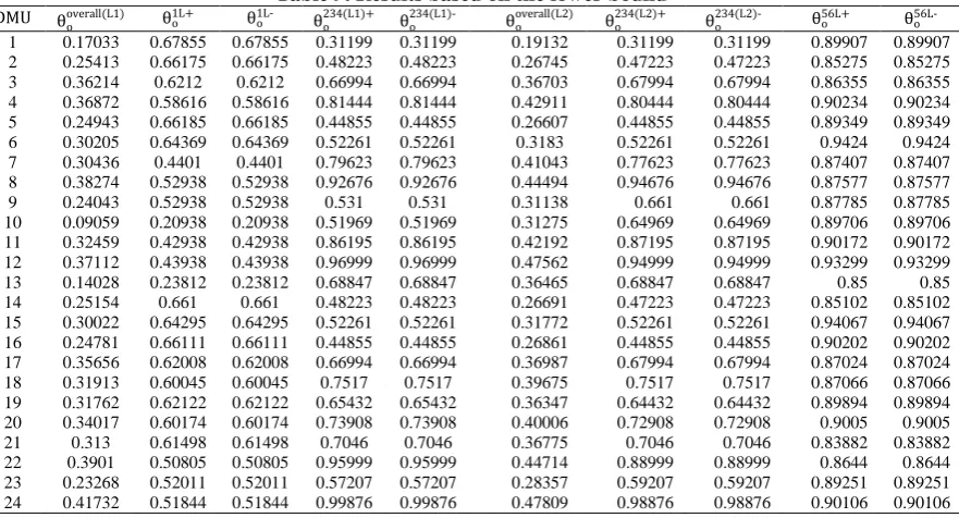
θ_ooverall(L)=max θ_o1L_{. θ}

o

234L_{. θ}

o

56L_{For which, we also implemented the heuristic approach for}

model (12). These results have been illustrated in the next part of the paper.

4. Case study description

(16)

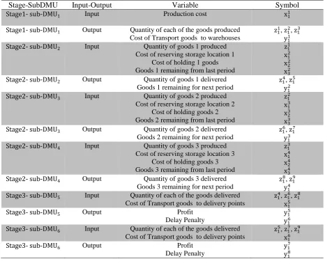
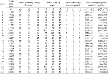
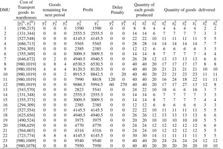
warehouse premises comprises of three warehouses within distances from each other, but in the same area; and a delivery point consisting of two locations, but situated at long distances from the warehouses. This factory produces three products and stores each product in a warehouse. We take this factory into consideration as a dynamic network for duration of 24 time periods and assume each time period as a DMU. In this network a number of outputs in the time period t in stage 2 are converted to a number of inputs to stage 2 during the time period t+1. The inputs-outputs of each DMU are defined as follows: the first stage is the production area and the inputs of the first stage are production costs (x₁1) for three goods. The intermediate measures between stage 1 and 2 are the quantity of each of the goods produced (z₁1, z₁2, z₁3). The undesirable output of the first stage is the cost of moving the goods from the production area to the warehouses ( y₁1). In the second stage we have three warehouses and additional inputs of each warehouse, which is the cost for reserving storage location (x₁2, x₁3, x₁4), the cost of holding goods in the warehouse (x₂2, x₂3, x₂4) and goods that have remained in the warehouse from the last period (x₃2, x₃3, x₃4). The desirable outputs of the warehouses in the second stage are defined by the goods remaining in each of the warehouses for the next period (y₁2, y₁3, y₁4). The intermediate measures between stages 2 and 3 are the quantity of goods delivered from each warehouse to every delivery point (z₁4, z₁5, z₁6, z₁7, z₁8, z₁9). The additional inputs in the third stage denotes the cost of moving goods from the warehouses to the delivery points (x₁5, x₁6). Finally, in the third stage the desirable and undesirable outputs are profits due to the sale of the goods (y₁5, y₁7) and the delay penalty (y₁6, y₁8), respectively. The inputs-outputs for each stage are summarized in Table (2).