https://doi.org/10.5194/essd-10-317-2018 © Author(s) 2018. This work is distributed under the Creative Commons Attribution 4.0 License.
Surface and top-of-atmosphere radiative feedback
kernels for CESM-CAM5
Angeline G. Pendergrass, Andrew Conley, and Francis M. Vitt
National Center for Atmospheric Research, Boulder, CO, 80305, USA
Correspondence:Angeline G. Pendergrass ([email protected])
Received: 13 September 2017 – Discussion started: 16 October 2017 Revised: 9 January 2018 – Accepted: 11 January 2018 – Published: 21 February 2018
Abstract. Radiative kernels at the top of the atmosphere are useful for decomposing changes in atmospheric radiative fluxes due to feedbacks from atmosphere and surface temperature, water vapor, and surface albedo. Here we describe and validate radiative kernels calculated with the large-ensemble version of CAM5, CESM1.1.2, at the top of the atmosphere and the surface. Estimates of the radiative forcing from greenhouse gases and aerosols in RCP8.5 in the CESM large-ensemble simulations are also diagnosed. As an application, feedbacks are calculated for the CESM large ensemble. The kernels are freely available at https://doi.org/10.5065/D6F47MT6, and accompanying software can be downloaded from https://github.com/apendergrass/cam5-kernels.
1 Introduction
A radiative feedback kernel is the radiative response to a small perturbation in, for example, temperature or water va-por. Radiative feedback kernels for the top of the atmosphere (TOA) are useful for decomposing changes in atmospheric radiative fluxes due to feedbacks from atmosphere and sur-face temperature, water vapor, and sursur-face albedo (Soden and Held, 2006). Radiative kernels at the surface or in the atmo-spheric column are useful for evaluating the radiative effect on precipitation (Pendergrass and Hartmann, 2014; Previdi, 2010).
Widely used TOA radiative kernels were calculated with the GFDL model (Soden and Held, 2006). Other kernels in-clude those from CAM3 (Shell et al., 2008) and more re-cently from the MPI-ESM-LR model (Block and Mauritsen, 2013). The only publicly available model-based surface ra-diative kernels are from ECHAM5 (Previdi, 2010) and MPI-ESM-LR, which is a more recent version of the ECHAM model (discussed in Fläschner et al., 2016). Reanalysis-based kernels generated with ERA-Interim and RRTM are also available (Huang et al., 2017). Not all kernels have been validated to test the accuracy to which total radiative fluxes from a model simulation can be recovered with kernel cal-culations; examples that have been validated against model calculations of radiative flux due to doubling of carbon
diox-ide include Shell et al. (2008), Block and Mauritsen (2013), and Huang et al. (2017).
Here we describe and validate radiative kernels calculated with CESM-CAM5 (Hurrell et al., 2013) for the top of the at-mosphere and the surface. These radiative feedback kernels were calculated with CESM version 1.1.2, the same as that used for the 40-member CESM large ensemble (Kay et al., 2015). The TOA kernels are an update from CAM3 (Shell et al., 2008). We also include estimates of radiative forcing due to greenhouse gases and aerosols in RCP8.5 in the CESM large-ensemble simulations, which are necessary for calcu-lating the cloud feedback using radiative kernels.
2 Calculations
-2 -1.5 -1 -0.5
0(e)Surface temperature kernel
SP -60 -30 EQ 30 60 NP -3
-2 -1
0(g) Surface albedo kernel All-sky temperature kernel
(a)
200
400
600
800
1000
Clear-sky temperature kernel
(c)
200
400
600
800
1000
All-sky LW moisture kernel
(b)
200
400
600
800
1000
Clear-sky LW moisture kernel
(d)
200
400
600
800
1000
-0.6 -0.5 -0.4 -0.3 -0.2 -0.1 0 0.1 0.2 0.3 0.4 0.5 0.6
All-sky SW moisture kernel
(f)
200
400
600
800
1000
Clear-sky SW moisture kernel
(h)
SP -60 -30 EQ 30 60 NP 200
400
600
800
1000
0 0.02 0.04 0.06 0.08 0.1
(W
m
–
2 K
–
1 )
(W
m
–
2 %
–
1 )
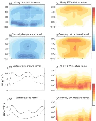
Figure 1.Top-of-atmosphere kernels from CESM1(CAM5). Zonal, annual-mean temperature, longwave moisture, and shortwave moisture kernels for all-sky and clear-sky. In panels(e)and(g)all-sky kernels are shown in solid lines and clear-sky kernels in dashed lines. The sign convention is positive downward.
were completed on NCAR’s Yellowstone computer system (Computational and Information Systems Laboratory, 2012).
2.1 Radiative kernels
Together, all calculations consumed approximately 200 000 core hours on NCAR’s Yellowstone supercomputer. The lim-iting factor for throughput is the size of PORT input data: 3-hourly 3-D temperature, moisture, and cloud fields; about 7.5 TB of disk space is needed to run 1 month of 3-hourly PORT calculations for each vertical level of each kernel, with 63 global radiative transfer computations per kernel month (control, surface temperature, and albedo each require 1
-5 -4 -3 -2 -1
0(e) Surface temperature kernel
SP -60 -30 EQ 30 60 NP
-3 -2 -1
0(g) Surface albedo kernel All-sky temperature kernel (a)
200 400 600 800 1000
Clear-sky temperature kernel (c)
200 400 600 800 1000
All-sky LW moisture kernel (b)
200 400 600 800 1000
Clear-sky LW moisture kernel (d)
200 400 600 800 1000
-1.2 -1 -0.8 -0.6 -0.4 -0.2 0 0.2 0.4 0.6 0.8 1 1.2
All-sky SW moisture kernel (f)
200 400 600 800 1000
Clear-sky SW moisture kernel (h)
SP -60 -30 EQ 30 60 NP
200 400 600 800 1000
-0.6 -0.4 -0.2 0
Latitude
Pressure (hPa)
(W
m
–
2 K
–
1 )
(W
m
–
2 %
–
1 )
(W
m
–
2
K
100
hPa
–
1
)
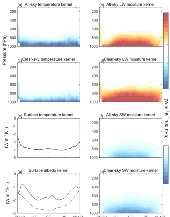
Figure 2.Surface kernels from CESM (CAM5). Zonal, annual-mean temperature, longwave moisture, and shortwave moisture kernels for all-sky and clear-sky cases. In panels(e)and(g)all-sky kernels are shown in solid lines and clear-sky kernels in dashed lines. The sign convention is positive downward.
TOA and Pendergrass and Hartmann (2014) for the atmo-spheric column.
2.1.1 Atmospheric temperature kernel
To calculate the atmosphere temperature kernel, we perturb the air temperature by 1 K in each hybrid sigma–pressure level at a time, at each grid cell for each 3-hourly instanta-neous field. Then we calculate the monthly mean, and take the difference of the TOA and surface radiative fluxes from the control in response to each perturbation. PORT is ad-justed so that the hygroscopic growth of aerosols is not af-fected by the modified temperatures and water vapor
con-centrations. The calculations are carried out in CESM’s hy-brid sigma-pressure vertical coordinate and have units of W m−2K−1level−1. These hybrid sigma-pressure radiative feedback kernels can be interpolated onto standard CMIP pressure levels (see the description of example code in Sect. 5), as is done for display purposes here; the atmospheric temperature kernel is shown in Fig. 1a, c for the TOA and Fig. 2a, c for the surface.
2.1.2 Surface temperature kernel
cal-culate the surface contribution to the temperature kernel, we perturb upwelling surface longwave radiation by an amount consistent with 1 K warming at constant effective emissivity. The surface temperature kernels are shown in Figs. 1, 2e.
2.1.3 Atmospheric moisture kernel
The atmospheric moisture kernel is constructed by per-turbing the mixing ratio on each hybrid sigma-pressure level by the amount that would result in constant relative-humidity moistening if there were a warming of 1 K. The saturation mixing ratio is calculated for each 3 h in-stantaneous state using the mixhum_ptd function in NCL (UCAR/NCAR/CISL/TDD, 2015), which calculates satura-tion with respect to liquid water following List (1951). Code to closely approximate the perturbation with monthly-mean fields using this NCL calculation is provided (dq1k.ncl). As with the temperature kernel, the mixing ratio does not change for the purpose of aerosol radiative properties (hygroscopic growth is held invariant). The moisture kernel is shown in Figs. 1, 2b, d, f, h.
2.1.4 Surface albedo kernel
The surface albedo kernel is the change in radiative flux for a 1 % change in surface albedo. The calculation is carried out by perturbing the direct and diffuse shortwave albedos, asdirandasdif, simultaneously by 1 % each. The sur-face albedo kernel is shown in Figs. 1, 2g.
2.2 Forcing
To estimate the radiative forcing, we reintegrate CESM for the year 2096, writing out the fields needed for PORT calcu-lations every 3 h. The baseline for the forcing calcucalcu-lations is the same 2006 control as the kernel calculations. The green-house gas and aerosol forcing are shown in Fig. 3.
2.2.1 Greenhouse gas forcing
We use the greenhouse gas concentrations (carbon dioxide, methane, CFCs, N2O, and ozone) from 2096 with the tropo-spheric temperature, mixing ratio, and other radiatively rel-evant fields from 2006. To account for stratospheric adjust-ment, we use the 2096 stratospheric temperature and water vapor mixing ratio in the calculation. The tropopause is de-fined as 100 hPa at the equator and 300 hPa at the poles and varies by cosine of latitude in between, following Soden and Held (2006). The resulting estimate approximates the radia-tive forcing following the definition of Myhre et al. (2013), though it includes adjustment of water vapor as well as tem-perature in the stratosphere.
2.2.2 Aerosol forcing
To calculate the aerosol forcing, we apply black carbon, sul-fate, secondary organic aerosol, primary organic matter, dust, sea salt, and aerosol temperature and mixing ratio from 2096 with temperature, mixing ratio, greenhouse gas, and all other fields from 2006, with no adjustments to the stratosphere. The resulting estimate is the instantaneous radiative forcing.
3 Validation
Radiative kernels enable a useful but approximate decompo-sition of the contributions to changes in radiative fluxes. Ap-plication of radiative kernels assumes that changes in radia-tive fluxes are linear with respect to changes in constituents, and that the response to changes in temperature and moisture at different vertical levels are independent. These assump-tions are not exactly met, even for clear-sky fluxes (Feldl and Roe, 2013). We undertake a validation exercise focused on quantifying the errors associated with these kernels com-pared to the climate-model-simulated changes in radiative flux they are targeted at.
First, we quantify the error of the kernel-estimated change in radiative flux of the ensemble member from which the ker-nels are computed. The changes in radiative flux associated with the temperature, water vapor, and albedo feedbacks are calculated using the changes in monthly-mean model fields, and then the change in radiative forcing is added. The global-mean modeled and kernel-estimated changes in radiative flux as well as the error in global mean and global-mean abso-lute error are documented in Table 1. For the global-mean absolute error, the change in annual-mean radiative fluxes is calculated, then the absolute value of the error for each ensemble member is calculated at each grid point, and fi-nally the global mean of this quantity is calculated. These error estimates include errors due to sampling every 3 h (in-stead of at each model time step) and due to the nonlinearity neglected by the kernel method. While we only document the changes in clear-sky radiative flux response in Table 1, the errors in all-sky radiative fluxes are exactly the same when cloud feedback is estimated using the adjusted cloud radiative effect method described in Soden et al. (2008). Er-rors in global-mean radiative flux change range from 0.1 to 0.8 Wm−2, while global-mean absolute errors range from 0.7 to 1.4 Wm−2. Errors in shortwave (SW) fluxes are smaller than for longwave (LW) fluxes.
(a) (b)
(c) (d)
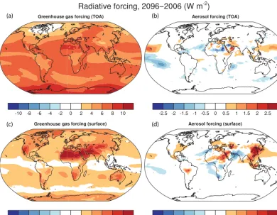
Figure 3.Radiative forcing. Net (LW+SW) radiative forcing under the RCP8.5 scenario diagnosed from CESM (CAM5) for greenhouse gases(a, c)and the direct aerosol radiative forcing(b, d)at the TOA(a, b)and surface(c, d).
Table 1.Top-of-atmosphere (TOA) and surface clear-sky radiative responses (Wm−2) for 2096–2006 from CESM1 large-ensemble member 1 (from which the kernels are derived) and the estimated radiative fluxes using the kernels and radiative forcing.
TOA Surface
LW SW LW SW
Member 1 response −1.3 3.1 9.5 −1.4 Kernel estimate −0.7 3.4 10.3 −1.2 Error of global mean 0.6 0.4 0.8 0.1 Global-mean abs. error 1.4 0.7 1.4 1.3
has more interannual variability than TOA SW and surface fluxes. The error of global-mean change in radiative flux is similar to member 1 for SW fluxes but larger for LW fluxes (0.9 Wm−2 at both the surface and TOA; not shown). The spatial pattern of ensemble-mean error is shown in Fig. 5. The LW errors, particularly for the surface, are large in the tropics. For the TOA, there are also substantial errors at high latitudes of both hemispheres. The largest errors in the SW are associated with sea-ice edges, the movement of which is not captured well by the kernel method. There are also
re-0 1 2
LW
Mean = 1.5
(a) SW
Mean = 0.8 (b)
2 10 20 30 40 0
1
2 Mean = 1.4
(c)
2 10 20 30 4 0
Mean = 1.3 (d)
Ensemble member
Global-mean absolute error (W m
-2)
TOA
Surface
Figure 4.Validation across ensemble members. Global-mean abso-lute error of kernel-estimated clear-sky radiative flux change from 2006 to 2096 for members 2–40 of the CESM1 large ensemble for LW(a, c)and SW(b, d)fluxes at the TOA(a, b)and surface(c, d).
gions of large error associated with tropical clouds, and at the TOA, there is a bias over Antarctica.
(a) (b)
(c) (d)
Figure 5.Spatial pattern of error. Mean error of kernel-estimated radiative flux change from 2006 to 2096 for members 2–40 of the CESM1 large ensemble for LW(a, c)and SW(b, d)fluxes at the TOA(a, b)and surface(c, d).
Planck Lapse rate
Water vapor Albedo
LW cloud SW clo
ud
Feedbacks -4
-2 0 2 4
[W
m
-2 -K]
CESM LENS (2071–2100)–(1976–2005)
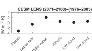
Figure 6.CESM large-ensemble kernels. Feedback calculation for the CESM 40-member large ensemble using the TOA kernels.
decompositions made with other radiative kernels from the literature in Sect. 4.
4 Application
Next we show a sample application of the kernels to the CESM large-ensemble simulations. In order to apply the ker-nels, one needs monthly changes in temperature, mixing ra-tio, and surface albedo as well as long-term mean water va-por mixing ratios to calculate the logarithm of water vava-por change (Soden et al., 2008). To calculate the cloud feedback, change in cloud radiative effect is also required. Then, the monthly-resolved kernels and changes in atmospheric state are convolved to obtain the changes in radiative flux compo-nents. Example code for applying the kernels is available at https://github.com/apendergrass/cam5-kernels.
Table 2.Comparison of TOA radiative feedbacks. TOA radiative feedbacks (Wm−2K−1) averaged over 40 CESM large-ensemble simulations diagnosed with CAM5 radiative kernels, compared against those from CMIP3 model simulations diagnosed with three different kernels as reported by Soden et al. (2008), and MPI-ESM-LR control state kernels and years 21–150 of abrupt carbon dioxide quadrupling simulations from the same model (Block and Maurit-sen, 2013).
Feedback Here Soden et al. Block and (2008) Mauritsen (2013)
Planck −3.2 −3.1 or−3.2 −3.19
Lapse rate −0.58 −1 −0.64
Water vapor 2.1 1.9 1.79
Albedo 0.51 0.3 0.48
Cloud 0.66 0.77 0.62
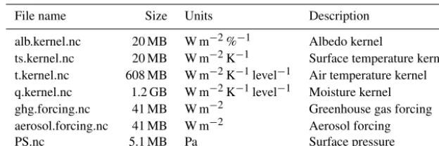
ensem-Table 3.Data files comprising the dataset.
File name Size Units Description
alb.kernel.nc 20 MB W m−2%−1 Albedo kernel
ts.kernel.nc 20 MB W m−2K−1 Surface temperature kernel t.kernel.nc 608 MB W m−2K−1level−1 Air temperature kernel q.kernel.nc 1.2 GB W m−2K−1level−1 Moisture kernel ghg.forcing.nc 41 MB W m−2 Greenhouse gas forcing aerosol.forcing.nc 41 MB W m−2 Aerosol forcing
PS.nc 5.1 MB Pa Surface pressure
ble member; then, the ensemble average is calculated. Re-sults are shown in Table 2 and Fig. 6.
Table 2 shows a comparison between feedback values cal-culated here and those diagnosed with other kernels and model simulations. Soden et al. (2008) report radiative feed-backs from 14 CMIP3 model simulations using three dif-ferent sets of radiative kernels from CAM3, GFDL, and CAWCR. The Planck response agrees closely. Water vapor and albedo feedbacks are both within 0.2 Wm−2K−1. The cloud feedback differs by only 0.1 Wm−2K−1, despite the fact that Soden et al. (2008) do not account for aerosol ra-diative forcing. The only notable disagreement is in the lapse rate feedback by 0.4 Wm−2K−1. Because the Planck feed-back agrees closely between the two calculations, the dif-ference is probably not due to the temperature kernel. In-stead, it may be caused by differing upper tropospheric tem-perature amplification between the CMIP3 and CESM large-ensemble simulations or due to underlying differences in the radiation codes. Block and Mauritsen (2013) report radiative feedbacks using MPI-ESM-LR kernels applied to abrupt car-bon dioxide quadrupling experiments with the same model (they compare kernels calculated from different base states and apply them to short transient response and more devel-oped long-timescale response; we compare with their control base-state kernels applied to long-timescale climate response because this is most similar to our application). There is re-markably close agreement for all feedbacks, excepting only the water vapor feedback. This could arise from the kernels or from the change in water vapor in the simulations.
5 Code and data availability
The provided dataset includes the four monthly-mean radia-tive kernels; atmospheric temperature, surface temperature, water vapor, and surface albedo; and radiative forcing from greenhouse gases and aerosols. Data are provided on the CESM hybrid-sigma grid for comparison with CESM sim-ulations. The dataset includes net all-sky and clear-sky radia-tive fluxes at both the top of the atmosphere and surface. The sign convention is the same as CESM’s: shortwave fluxes are positive downward, and longwave fluxes are positive upward. Sample temperature, moisture, surface radiative fluxes, and
surface pressure are also included, as well as sample code to facilitate use of the kernels.
The data and code to calculate TOA temperature, water vapor, and albedo feedbacks are available for immediate download at https://zenodo.org/record/997902 (though without directory structure) and through ESGF at https://www.earthsystemgrid.org/dataset/ucar.cgd.ccsm4. cam5-kernels.html (Pendergrass, 2017a). The files included are listed in Table 3. Additional software tools – to regrid the kernels to pressure levels (including CMIP standard levels), and calculate TOA Planck, lapse rate, and cloud feedbacks – are available at https://doi.org/10.5281/zenodo.997899 (Pen-dergrass, 2017b).
6 Path forward
There is room to improve the accuracy of these and other radiative kernels. Future work could explore new sampling strategies to capture both the diurnal cycle and interannual variability (which would be particularly important for re-gional applications), directly compare different kernels, and quantify the radiative forcing in climate simulations.
Competing interests. The authors declare that they have no con-flict of interest.
Edited by: David Carlson
Reviewed by: two anonymous referees
References
Block, K. and Mauritsen, T.: Forcing and feedback in the MPI-ESM-LR coupled model under abruptly quadru-pled CO2, J. Adv. Model. Earth Syst., 5, 676–691, https://doi.org/10.1002/jame.20041, 2013.
Computational and Information Systems Laboratory: Yellowstone: IBM iDataPlex System (NCAR Community Computing), avail-able at: http://n2t.net/ark:/85065/d7wd3xhc, 2012.
Conley, A. J., Lamarque, J.-F., Vitt, F., Collins, W. D., and Kiehl, J.: PORT, a CESM tool for the diagnosis of radiative forcing, Geosci. Model Dev., 6, 469–476, https://doi.org/10.5194/gmd-6-469-2013, 2013.
DeAngelis, A. M., Qu, X., Zelinka, M. D., and Hall, A.: An obser-vational radiative constraint on hydrologic cycle intensification, Nature, 528, 249–53, https://doi.org/10.1038/nature15770, 2015. Feldl, N. and Roe, G. H.: The nonlinear and nonlocal na-ture of climate feedbacks, J. Climate, 26, 8289–8304, https://doi.org/10.1175/JCLI-D-12-00631.1, 2013.
Fläschner, D., Mauritsen, T., and Stevens, B.: Understanding the in-termodel spread in global-mean hydrological sensitivity, J. Cli-mate, 29, 801–817, https://doi.org/10.1175/JCLI-D-15-0351.1, 2016.
Huang, Y., Xia, Y., and Tan, X.: On the pattern of CO2radiative forcing and poleward energy transport, J. Geophys. Res.-Atmos., 122„ 10578–10593, https://doi.org/10.1002/2017JD027221, 2017.
Hurrell, J. W., Holland, M. M., Gent, P. R., Ghan, S., Kay, J. E., Kushner, P. J., Lamarque, J. F., Large, W. G., Lawrence, D., Lindsay, K., Lipscomb, W. H., Long, M. C., Mahowald, N., Marsh, D. R., Neale, R. B., Rasch, P., Vavrus, S., Vertenstein, M., Bader, D., Collins, W. D., Hack, J. J., Kiehl, J., and Mar-shall, S.: The Community Earth System Model: A framework for collaborative research, B. Am. Meteorol. Soc., 94, 1339–1360, https://doi.org/10.1175/BAMS-D-12-00121.1, 2013.
Iacono, M. J., Delamere, J. S., Mlawer, E. J., Shephard, M. W., Clough, S. A., and Collins, W. D.: Radiative forcing by long-lived greenhouse gases: Calculations with the AER ra-diative transfer models, J. Geophys. Res.-Atmos., 113, 2–9, https://doi.org/10.1029/2008JD009944, 2008.
Ingram, W.: A very simple model for the water vapour feed-back on climate change, Q. J. Roy. Meteorol. Soc., 136, 30–40, https://doi.org/10.1002/qj.546, 2010.
Kay, J. E., Deser, C., Phillips, A., Mai, A., Hannay, C., Strand, G., Arblaster, J. M., Bates, S. C., Danabasoglu, G., Edwards, J., Holland, M., Kushner, P., Lamarque, J. F., Lawrence, D., Lindsay, K., Middleton, A., Munoz, E., Neale, R., Oleson, K., Polvani, L., and Vertenstein, M.: The Community Earth Sys-tem Model (CESM) large ensemble project?: A community re-source for studying climate change in the presence of inter-nal climate variability, B. Am. Meteorol. Soc., 96, 1333–1349, https://doi.org/10.1175/BAMS-D-13-00255.1, 2015.
List, R. J. (Ed.): Smithsonian meteorological tables, 6th edn., The Smithsonian Institution, Washington, 1951.
Myhre, G., Shindell, D., Bréon, F.-M., Collins, W., Fuglestvedt, J., Huang, J., Koch, D., Lamarque, J.-F., Lee, D., Mendoza, B., Nakajima, T., Robock, A., Stephens, G., Takemura, T., and Zhang, H.: Anthropogenic and Natural Radiative Forcing, in Cli-mate Change 2013: The Physical Science Basis. Contribution of Working Group I to the Fifth Assessment Report of the Intergov-ernmental Panel on Climate Change, edited by: Stocker, T. F., Qin, D., Plattner, G.-K., Tignor, M., Allen, S. K., Boschung, J., Nauels, A., Xia, Y., Bex, V., and Midgley, P. M., Cambridge Uni-versity Press, Cambridge, United Kingdom and New York, NY, USA, 2013.
Pendergrass, A. G.: CAM5 Radiative Kernels, UCAR/NCAR Earth Syst. Grid, https://doi.org/10.5065/D6F47MT6, 2017a.
Pendergrass, A. G.: CESM CAM5 Kernel Software, Zenodo, https://doi.org/10.5281/zenodo.997899, 2017b.
Pendergrass, A. G. and Hartmann, D. L.: The atmospheric energy constraint on global-mean precipitation change, J. Climate, 27„ 757–768, https://doi.org/10.1175/JCLI-D-13-00163.1, 2014. Previdi, M.: Radiative feedbacks on global precipitation,
En-viron. Res. Lett., 5, 25211, https://doi.org/10.1088/1748-9326/5/2/025211, 2010.
Shell, K. M., Kiehl, J. T., and Shields, C. A.: Using the radia-tive kernel technique to calculate climate feedbacks in NCAR’s Community Atmospheric Model, J. Climate, 21, 2269–2282, https://doi.org/10.1175/2007JCLI2044.1, 2008.
Soden, B. J. and Held, I. M.: An Assessment of Climate Feedbacks in Coupled Ocean – Atmosphere Models, J. Climate, 19, 3354– 3360, https://doi.org/10.1175/JCLI9028.1, 2006.
Soden, B. J., Held, I. M., Colman, R. C., Shell, K. M., Kiehl, J. T., and Shields, C. A.: Quantifying climate feed-backs using radiative kernels, J. Climate, 21, 3504–3520, https://doi.org/10.1175/2007JCLI2110.1, 2008.