Removing low-frequency artefacts from Datawell DWR-G4 wave buoy measurements

(1)

www.geosci-instrum-method-data-syst.net/5/17/2016/ doi:10.5194/gi-5-17-2016

Removing low-frequency artefacts from Datawell DWR-G4 wave

buoy measurements

J.-V. Björkqvist1, H. Pettersson1, L. Laakso1,2, K. K. Kahma1, H. Jokinen1, and P. Kosloff1 1_{Finnish Meteorological Institute, Helsinki, Finland}

2_{Unit for Environmental Sciences and Management, North-West University, Potchefstroom, Republic of South Africa}

Correspondence to: J.-V. Björkqvist (jan-victor.bjorkqvist@fmi.fi)

Received: 11 September 2015 – Published in Geosci. Instrum. Method. Data Syst. Discuss.: 3 November 2015 Revised: 8 January 2016 – Accepted: 14 January 2016 – Published: 5 February 2016

Abstract. In this study we describe a previously unreported error in the vertical-displacement time series made with GPS-based Datawell DWR-G4 wave buoys and introduce a simple method to correct the resulting wave spectra. The artefact in the time series is found to resemble a sawtooth wave, which produces an erroneous trend following anf−2 power law in frequency space. The correction method quanti-fies the amount of erroneous trend below a certain maximum frequency and removes the spurious energy from all frequen-cies assuming the above-mentionedf−2power law. The pre-sented correction method is validated against an experimen-tal field test, and its impact on the measured significant wave height is quantified. The method’s sensitivity to the choice of the maximum frequency is also briefly discussed.

1 Introduction

Surface wind waves are an important factor for the safety and efficiency of marine traffic, seaborne operations and coastal structures. Short-term observations are well suited to map the wave field and to support wave model development, espe-cially at complex shorelines. Currently the large wave buoys utilising accelerometers to measure the pitch, heave and roll of the buoy are considered highly reliably instruments for op-erational measurements. Nevertheless, there also exist sev-eral different technologies that use a GPS receiver to mea-sure the displacement of the wave buoy, which have all been proven to be sufficiently accurate in a majority of situations (Herbers et al., 2012). Especially the technique using the Doppler shift of the GPS signal to measure the velocity of the wave buoy has been shown to produce excellent results

when compared to an accelerometer-based Datawell Direc-tional Waverider (DWR) (de Vries et al., 2003; Jeans et al., 2003).

The small size of the GPS receiver enables the con-struction of smaller and more robust wave buoys like the Datawell DWR-G4, which is only 40 cm in diameter. Ac-cording to our experience these smaller buoys are practical and cost-efficient, especially for short measurements (e.g. Tuomi et al., 2014) where they can be moored or deployed as floating devices.

In this paper we describe an observed error reading in the G4 measurements, suggest an easy and automated corrective method and discuss the accuracy and limitations of the cor-rection based on experiments.

2 The artefact

(2)

Table 1. Mean and extreme difference in significant wave height of the G4 wave buoy when compared to the DWR wave buoy. The significant wave height is calculated for both the entire frequency range and for the low-frequency part of the spectra only. Two corrections are made using different maximum frequencies to quantify the erroneous energy. Values are calculated from data where erroneous energy was present (i.e. the correction by the method was at least 0.1 m).

1Hs(<0.1 Hz) 1Hs

G4 vs. DWR mean (m) extreme (m) mean (m) extreme (m)

Uncorrected 0.8 1.8 0.2 0.7

Correction usingf <0.07 Hz 0.0 0.2 −0.1 −0.5 Correction usingf <0.04 Hz 0.0 0.3 −0.1 −0.5

0 200 400 600 800 1000 1200 1400 1600 1800 −2

−1 0 1 2

t (s)

z (m)

0 200 400 600 800 1000 1200 1400 1600 1800 −2

−1 0 1 2

t (s)

z (m)

Figure 1. Artefact observed in a G4 buoy. Vertical displacement measured with the G4 buoy with the artificial jumps indicated with red arrows (top panel). Vertical-displacement time series of the mea-surements by an accelerometer-based DWR made in close proxim-ity and during roughly the same time (bottom panel). The distance between the two devices were about 900 m.

are caused by atmospheric conditions. Even if the receiving unit is functioning properly, any disturbances in the propaga-tion of the signal could lead to an incorrect determinapropaga-tion of the velocity of the wave buoy, since the wave buoy relies on the measurement of the Doppler shift. However, we have not found any definite connection between the magnitude of the artefact and any local meteorological parameter (wind speed, humidity etc.).

0 100 200 300 400 500 −2

−1 0 1 2

Time (s)

Vertical displacement (m)

(a)

0 0.1 0.2 0.3 0.4

0 1 2 3 4 5

Frequency (Hz)

Variance density (m

2Hz

−1

(b)

0 100 200 300 400 500 −2

−1 0 1 2

Time (s)

(c)

0 0.1 0.2 0.3 0.4

0 1 2 3 4 5

Frequency (Hz)

Variance density (m

2Hz

−1

) (d)

0 100 200 300 400 500 −2

−1 0 1 2

Time (s)

(e)

0 0.1 0.2 0.3 0.4

0 1 2 3 4 5

Frequency (Hz)

Variance density (m

2Hz

−1

) (f)

Figure 2. A schematic illustration of signal and the frequency re-sponse of a clean time series (a–b), a sawtooth wave (c–d) and the combined time series (e–f). The wave spectrum (f) of the combined signal is just a superimposition of the wave spectra (b, d) of the individual signals.

3 The wave spectrum and the correction method 3.1 The wave spectrum

(3)

wave periods, are extensively used both for operational and for research purposes.

The 1-D wave spectrum is the power density spectrum of the vertical displacement. Theoretically it is defined as the Fourier transform of the autocovariance function of the ver-tical displacement, but in practice it is usually calculated di-rectly form the vertical displacement by using the fast Fourier transform (FFT) (see e.g. Bendat and Piersol, 2010). All the wave spectra in this study are the ones calculated on board the wave buoys by taking the Fourier transform piecewise from the time series, but the correction technique we propose is not dependant on the method used to calculate the wave spectrum. For a more detailed description of the method used on board the buoys the reader is referred to the Datawell man-ual (Datawell BV, 2014).

A schematic illustration of the frequency responses of the relevant signals is shown in Fig. 2. The power density spec-trum of a sawtooth wave follows an f−2 frequency power law, which is not limited by any upper frequency. Solu-tions depending on discarding all data from the spectra be-low a cut-off frequency will therefore not be sufficient, even though it has previously been used to remove erroneous low-frequency data of a different type (Joodaki et al., 2013).

The observed error reading in Fig. 1 has the shape of a sawtooth wave. The correction method presented in this pa-per will therefore be based on the known frequency response of the artefact.

3.2 The correction method

To quantify the amount of spurious energy, we will first need to determine a frequency interval that we can assume to con-tain pure erroneous trend. As a first guess for the upper limit we took 0.07 Hz. This choice was based on our long experi-ence that there is practically no physically meaningful wave data below that frequency in the Baltic Sea (e.g. Kahma, 1981; Kahma et al., 2003; Pettersson, 2004; Tuomi, 2008; Tuomi et al., 2011). For the purpose of our calculations we can therefore assume that frequencies below 0.07 Hz contain only pure erroneous trend. The choice of frequency interval for e.g. a different geographical location will have to be made based on the knowledge of the local wave field. The effect the chosen maximum frequency has on our results is further discussed in Sect. 5.

Because of the underlying f−2power law the erroneous trend will have a constant value if the spectrum is scaled by a factor off2. We will then calculate the mean value of the scaled trend from frequencies below 0.07 Hz and remove it from the entire spectrum prior to de-scaling. A schematic picture of the de-trending process is shown in Fig. 3.

In practice the trend will not always be smooth. The varia-tions around the mean value may cause small positive and negative residuals even below the chosen maximum fre-quency of 0.07 Hz. As an additional step, we will remove any residuals below 0.07 Hz (usually very small) and set possible

negative values to zero (because the original spectral file is always strictly non-negative). The first step is mostly cos-metic and the latter practical. We want to stress that the real correction of the spectrum is made by the removing of the mean trend.

4 Experimental

We at the Finnish Meteorological Institute1 (FMI) have observed waves in the Baltic Sea since the 1970s both campaign-based (e.g. Kahma, 1981; Pettersson, 2004; Tuomi et al., 2014) and operationally (e.g. Pettersson and Jöns-son, 2004; Tuomi, 2008). The measurements have been conducted with various instruments, including wave buoys, acoustic Doppler current profilers (ADCPs) and wave staffs. Our operational measurements are made with wave buoys equipped with accelerometer-based sensors, but we have also used GPS-based wave buoys for additional shorter measure-ments since 2006.

To test the correction method described in Sect. 3, we de-ployed a GPS-based Datawell DWR-G4 (henceforth, “the G4”) in close proximity to FMI’s operational accelerometer-based Directional Waverider (“the DWR”) in the centre of the Gulf of Finland (Fig. 4). The measurement period for the G4 was 4–20 May 2015, during which time the significant wave height measured by the DWR ranged from 0.1 to 2.9 m.

Both wave buoys use a 0.78 s sampling time to measure the 1600 s time series from which they calculate the wave spec-tra every half hour. The specspec-tra from both buoys have a fre-quency range of 0.025–0.580 Hz with a resolution of 0.01 Hz (0.005 Hz for frequencies under 0.1 Hz).

The significant wave height is defined as Hs=4 √

m0, wherem0is the zeroth moment (i.e. the integral) of the wave spectrum. The integral of the wave spectrum is also the vari-ance of the vertical-displacement time series.

5 Results

The variance density (m2Hz−1) of each frequency bin from the G4 wave buoy was compared to those of the DWR for the whole data set. Figure 5 shows the bias of the original and corrected G4 spectra compared to the reference data from the DWR. We can see that the original G4 data have a pos-itive bias following the expectedf−2 power law, which is no longer visible after the correction. The correction method applied to the, presumably correct, DWR spectra resulted in only negligible changes (not shown).

The maximum reduction in significant wave height when using the correction method was 1.0 m (a reduction from 3.3 to 2.3 m). To visualise the occurrence frequency of the anomaly in our field data, we plotted the difference in signif-icant wave height from the G4 buoy before and after the use

(4)

0 0.1 0.2 0.3 0.4 0 1 2 3 4 5 6 Spectrum Artefact True spectrum Frequency (Hz) m 2 Hz −1 (a)

0 0.1 0.2 0.3 0.4 0 0.02 0.04 0.06 0.08 0.1 0.12 0.14 Spectrum Artefact Corrected spec. Frequency (Hz) m 2 Hz −1 ⋅ Hz 2 (b)

0 0.1 0.2 0.3 0.4 0 1 2 3 4 5 6 True spectrum Corrected spec. Frequency (Hz) m 2 Hz −1 (c)

Figure 3. A schematic illustration of the approach to correct a wave spectrum with erroneous trend. A hypothetical spectrum containing erroneous low-frequency energy is shown in (a). The method scales the spectrum by multiplication off2to reveal the power law of the erroneous trend (b). The level of the trend (dashed magenta) is determined from the low frequencies where the scaled spectrum is constant, and the trend is removed from all frequencies. The de-scaled spectrum is shown in (c).

24˚ 25˚ 26˚

59˚30' 60˚00'

0 10 20 30

km -90 _-70 -70 -70 -70 -70 -70 -70 -70 -50 -50 -50 -50 -50 -50 -50 -50 -50 -50 -50 -30 -30 -30 -30 -30 -30 -30 -30 -30 -30 -30 -10 -10 -10 -10 -10 -10 -10 -10 -10 -10 -10 0 0 0 0 0 0 0 0 0 0 0

24˚ 25˚ 26˚

59˚30' 60˚00'

24˚ 25˚ 26˚

59˚30' 60˚00'

Tallinn

Helsinki

DWR G4

24˚ 25˚ 26˚

59˚30' 60˚00'

24˚ 25˚ 26˚

59˚30' 60˚00'

24˚ 25˚ 26˚

59˚30' 60˚00'

24˚ 25˚ 26˚

59˚30' 60˚00'

24˚ 25˚ 26˚

59˚30' 60˚00'

Figure 4. The location of the deployed wave buoys in the Gulf of Finland. The operational DWR (red circle) is anchored at a depth of 62 m at 59◦57.900N, 025◦14.110E. The G4 (yellow circle) was anchored at a similar depth at 59◦57.500N, 025◦14.570E.

of the correction method in a logarithmic histogram (Fig. 6). The relative value is defined as the difference between the original and corrected significant wave height normalised by the original significant wave height.

Four situations with an increasing amount of erroneous trend are shown in Fig. 7. The first case (a) illustrates that the method does not interfere with an uncorrupted spectrum. In the three following cases the erroneous trend continues above the maximum frequency used to quantify the spurious

0 0.1 0.2 0.3 0.4 0.5 0.6

−0.4 −0.3 −0.2 −0.1 0 0.1 0.2 0.3 0.4 f (Hz) E(f) m 2 Hz −1 G4 Corrected G4 Max. frequency

Figure 5. Bias of the power spectrum of the G4 data before and after the correction compared to the reference data from the DWR. The distribution is based on 3 weeks of data.

energy (0.07 Hz), but even these higher frequencies are cor-rected as a comparison to the DWR spectra reveals.

(5)

0.0 0.2 0.4 0.6 0.8 1.0 10−2

10−1 100 101 102

Percentage of cases

Absolute H s error (m)

0.00 0.08 0.16 0.24 0.32 0.40 10−2

10−1 100 101 102

Percentage of cases

Relative H s error

Figure 6. The difference in significant wave height when calculated from the original and corrected wave spectra measured by the G4 wave buoy. Absolute values (left panel) and relative values (right panel). The relative value is the difference between the original and corrected significant wave height normalised by the original significant wave height.

f (Hz)

0 0.1 0.2 0.3 0.4 0.5 0.6

E(f) m

2Hz

-1

0 0.5 1 1.5 2 2.5 3

G4 Corrected G4 DWR Max. frequency

H s (m) 1.19 (G4) 1.18 (Corr. G4) 1.22 (DWR)

(a)

f (Hz)

0 0.1 0.2 0.3 0.4 0.5 0.6

E(f) m

2Hz

-1

0 0.5 1 1.5 2 2.5 3

H s (m) 1.28 (G4) 1.21 (Corr. G4) 1.21 (DWR)

(b)

f (Hz)

0 0.1 0.2 0.3 0.4 0.5 0.6

E(f) m

2Hz

-1

0 0.5 1 1.5 2 2.5 3

H_s (m) 1.84 (G4) 1.71 (Corr. G4) 1.73 (DWR)

(c)

f (Hz)

0 0.1 0.2 0.3 0.4 0.5 0.6

E(f) m

2Hz

-1

0 0.5 1 1.5 2 2.5 3

H_s (m) 1.67 (G4) 1.36 (Corr. G4) 1.39 (DWR)

(d)

Figure 7. The power law method applied to four example wave spectra from May 2015 with different amount of erroneous trend present. The significant wave heightHsis calculated for the original G4 data, the corrected G4 data and the DWR data.

Because of the small size of the Baltic Sea, we were able to use a relatively high maximum frequency of 0.07 Hz (i.e. 14 s wave period) as an initial guess for an appropriate value. However, one cannot generally assume that there are no physically relevant wave data below 0.07 Hz, which calls for a lower upper limit when quantifying the trend. To test the sensitivity of the method, we repeated the calculations using a maximum frequency of 0.04 Hz (i.e. 25 s wave period).

(6)

Frequency (Hz)

0 0.1 0.2 0.3 0.4 0.5 0.6

m

2Hz

-1

0 1 2 3

G4 DWR Max. frequency

(a)

Frequency (Hz)

0 0.1 0.2 0.3 0.4 0.5 0.6

m

2Hz -1·

Hz

2

0 0.01 0.02 0.03 0.04 0.05 0.06 0.07

G4 Corrected G4 Artefact (mean) Max. frequency

(b)

Frequency (Hz)

0 0.1 0.2 0.3 0.4 0.5 0.6

m

2Hz

-1

0 1 2 3

Corrected G4 DWR Max. frequency

(c)

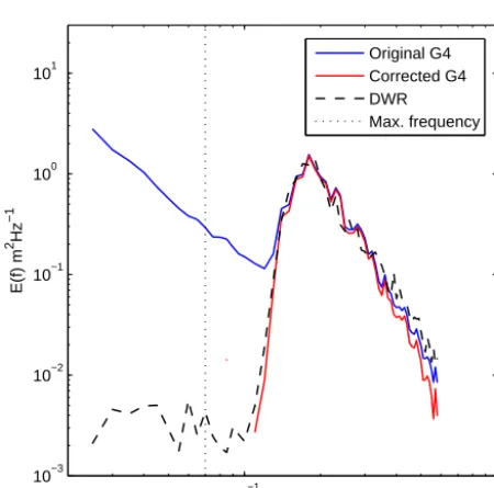
Figure 8. An example of the correction applied to a wave spectrum from a G4 wave buoy (14 May 2015). The original spectrum (a), the spectrum scaled byf2and the level of the mean trend (b) and the corrected de-scaled spectrum (c). The spectrum from the DWR is shown for comparison. The dotted line indicates the maximum frequency (0.07 Hz) used to determine the level of the erroneous trend.

10−1 100

10−3 10−2 10−1 100 101

f (Hz)

E(f) m

2Hz

−1

Original G4 Corrected G4 DWR Max. frequency

Figure 9. The example spectra from Fig. 7d shown on a logarithmic scale for illustrative purposes. Note that the values that are in set to zero in the corrected spectra cannot be displayed on the logarithmic scale.

is easily explained by the fact that the level of the trend is equally well defined below 0.04 Hz (Fig. 8b).

To better illustrate even the small differences between the original and corrected spectra, we plotted the already-presented case of Fig. 7d on a logarithmic scale (Fig. 9). A trend following an f−2 power law should be linear in a logarithmic plot, which is indeed the case. The figure also illustrates that a slight overcorrection is possible for the high-est frequencies (0.40–0.58 Hz), where the trend becomes the same order of magnitude as the spectrum. This can be due to

other small low-frequency errors that contribute to the spec-trum below 0.07 Hz, which in turn will make the correction slightly too large. However, this possible overcorrection is inconsequential for the calculation of any basic parameters, such as the significant wave height. Even though we recom-mend the corrected data to be carefully checked when used in advanced wave studies, the method presented in this paper is suitable to be implemented as an automated approach for e.g. operational applications.

6 Conclusions

In this paper we introduce a simple automated method to correct Datawell DWR-G4 data for an error observed in the lower frequencies. This error is caused by a sawtooth-like artefact in the time domain and thus follows anf−2power law in the frequency domain (Figs. 1 and 2). We have con-cluded that the artefact in the time domain is caused by the use of the Doppler shift technology, but we are not aware of any previous reports of this kind of behaviour.

The basic idea of the method is to calculate the level of the erroneous trend from the frequency bins we know to lack physically relevant information (we used 0.07 Hz as an upper limit for the Baltic Sea) and then remove it for the whole frequency range (see Fig. 3 for a schematic overview of the method).

(7)

accu-racy of the observations even if only integrated parameters, such as significant wave height, are considered.

The results presented in Table 1 show that the method pro-duces the same results if the level of the erroneous trend is quantified only below 0.04 Hz. This robustness increases the usability of the correction method for different physical and geographical conditions.

Although the correction is generally concentrated on the low-frequency part of the spectrum, there is a possibility of a small overcorrection of the high-frequency tail (>0.4 Hz) (Fig. 9). Luckily, these minor differences are not important for basic applications that use only integrated parameters. Nonetheless, the corrected data should be analysed if they are to be used for more advanced wave research.

Data availability

(8)

Appendix A: Code for correcting wave buoy spectra A simple MATLAB code for correcting data from Datawell G4 wave buoys.

function S_DT=detrend_wavespec(f,S,f_max)

S_scaled=S.*f.^2; % Scale the spectrum with f^2

bin_max=find(f<=f_max,1,’last’); % Select the bins used to

% calculate the trend

Trend=mean(S_scaled(1:bin_max)); % Calculate mean scaled trend

S_scaled=S_scaled-Trend; % Remove mean scaled trend

S_scaled(1:bin_max)=0; % These freq. bins did not contain any

% real information

S_scaled=max(S_scaled,0); % Force to positive values

(9)

The Supplement related to this article is available online at doi:10.5194/gi-5-17-2016-supplement.

Acknowledgements. We are grateful to senior scientist Kristian Spilling from the Finnish Environment Institute for arranging the time for our measurements during his cruise on RV Aranda on such short notice.

Edited by: C. Waldmann

References

Ashton, I. G. C. and Johanning, L.: On errors in low frequency wave measurements from wave buoys, Ocean Eng., 95, 11–22, doi:10.1016/j.oceaneng.2014.11.033, 2015.

Bendat, J. S. and Piersol, A. G.: Random Data: Analysis and Mea-surement Procedures, 4th Edn., Wiley Series in Probability and Statistics, Hoboken, New Jersey, 2010.

Datawell BV: Datawell Waverider Manual DWR4, avail-able at: http://datawell.xcess-5.xec.nl/Portals/0/Documents/ Manuals/datawell_manual_dwr4_2014-11-10.pdf (last access: 10 September 2015), 2014.

de Vries, J. J., Waldron, J., and Cunningham, V.: Field tests of the New Datawell DWR-G GPS wave buoy, Sea Technol., 44, 50– 55, 2003.

Herbers, T. H. C., Jessen, P. F., Janssen, T. T., Colbert, D. B., and MacMahan, J. H.: Observing ocean surface waves with GPS-tracked buoys, J. Atmos. Ocean. Tech., 29, 944–959, doi:10.1175/JTECH-D-11-00128.1, 2012.

Jeans, G., Bellamy, I., de Vries, J. J., and van Weer, P.: Sea trial of the new datawell GPS directional waverider, in: Proceeding of the IEEE/OES Seventh Working Conference, San Diego, CA, USA, 145–147, doi:10.1109/CCM.2003.1194302, 2003. Joodaki, G., Nahavandchi, H., and Cheng, K.: Ocean wave

mea-surements using GPS buoys, J. Geodet. Sci., 3, 163–172, doi:10.2478/jogs-2013-0023, 2013.

Kahma, K. K.: A study of the growth of the wave spectrum with fetch, J. Phys. Oceanogr., 11, 1504–1515, doi:10.1175/1520-0485(1981)011<1503:ASOTGO>2.0.CO;2, 1981.

Kahma, K. K., Pettersson, H., and Tuomi, L.: Scatter diagram wave statistics from the Northern Baltic Sea, Rep. Ser. Finnish Inst. Mar. Res., 49, 15–32, 2003.

Pettersson, H.: Wave Growth in a Narrow Bay, Finnish Institute of Marine Research – Contributions, Helsinki, Finland, 1–33, 2004. Pettersson, H. and Jönsson, A.: Wave climate in the northern Baltic Sea in 2004, available at: http://www.helcom.fi/baltic-sea-trends/ environment-fact-sheets/ (last access: 10 September 2015), 2004.

Tuomi, L.: The accuracy of FIMR wave forecasts in 2002–2005, Rep. Ser. Finnish Inst. Mar. Res., 63, 7–17, 2008.

Tuomi, L., Kahma, K. K., and Pettersson, H.: Wave hindcast statis-tics in the seasonally ice-covered Baltic Sea, Boreal Environ. Res., 16, 451–472, 2011.