Determinantal Reinforcement Learning

(1)

The Thirty-Third AAAI Conference on Artificial Intelligence (AAAI-19)

Determinantal Reinforcement Learning

Takayuki Osogami, Rudy Raymond

IBM Research - Tokyo Tokyo, Japan

Abstract

We study reinforcement learning for controlling multiple agents in a collaborative manner. In some of those tasks, it is insufficient for the individual agents to take relevant ac-tions, but those actions should also have diversity. We propose the approach of using the determinant of a positive semidefi-nite matrix to approximate the action-value function in rein-forcement learning, where we learn the matrix in a way that it represents the relevance and diversity of the actions. Ex-perimental results show that the proposed approach allows the agents to learn a nearly optimal policy approximately ten times faster than baseline approaches in benchmark tasks of multi-agent reinforcement learning. The proposed approach is also shown to achieve the performance that cannot be achieved with conventional approaches in partially observ-able environment with exponentially large action space.

Introduction

We study the problem of learning to control multiple agents in a collaborative manner. For example, players of a team want to learn from their experience how to collaboratively play to win a game, or one might want to learn to control multiple robots to accomplish a task that cannot be handled by a single robot. For some of those multi-agent tasks, it is important for the agents to take not only individually rele-vant but also collectively diverse actions. For example, play-ers of a defensive team should guard relevant and divplay-erse areas (i.e., zone defense) or relevant and diverse players of the other team (i.e., man-to-man defense).

Even when we have central control, multi-agent reinforce-ment learning is hard due to exponentially many possible combinations of actions. The simple approach of handling the combination of actions as if it is an action of a hypothet-ical single agent (or a team) does not scale with increased number of agents. It is also undesirable to let each agent greedily take an action without consideration of others.

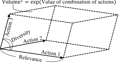
We propose to use the determinant of a matrix to approx-imate the action-value function in reinforcement learning where the combination of relevant and diverse actions tends to have high value (see Figure 1). Each action is character-ized by a feature vector, whose length represents the rele-vance of that action at a state, and the angle between two

Volume2_{= exp(Value of combination of actions)}

Figure 1: The logarithm of the squared volume of the paral-lelepiped defined by the feature vectors of actions represents the value of the combination of those actions.

feature vectors represents the similarity between two actions at that state. The feature vector depends on the state. A set of feature vectors then defines a parallelotope whose squared volume is given by the determinant of the Gram matrix of those feature vectors. More specifically, the value of a com-bination of actions at a state is given by the logarithm of the determinant (log-determinant) of a principal submatrix of a positive semidefinite matrix (kernel), where the prin-cipal submatrix is specified by the actions, and the kernel depends on the state.

The proposed approach can deal with partial observability by letting the kernel depend on the history of observations (of non-Markovian states). The special case of a history-dependent diagonal kernel reduces to the standard approach of representing the action-value function with a time-series model such as a recurrent neural network (Hausknecht and Stone 2015), vector autoregressive models, and dy-namic Boltzmann machines (Osogami and Otsuka 2015; Osogami 2017). Our approach can thus be seen as adding a differential “determinantal layer” to the output of a neural network.

(2)

ap-proximately 10 times faster than baseline approaches (Sal-lans and Hinton 2001; 2004; Heess, Silver, and Teh 2013; Sallans 2002), where free energy of a restricted Boltzmann machine (RBM) is used as a functional approximator. De-terminantal SARSA also finds nearly optimal policy for stochastic policy tasks, substantially outperforming those baseline approaches, due to its capability of effectively deal-ing with partial observability.

Our contributions can be summarized as follows. First, we introduce the idea of using the determinant in reinforcement learning to approximate the action-value function. Second, we derive specific learning rules of Determinantal SARSA. Finally, we demonstrate the effectiveness of Determinantal SARSA in reinforcement learning where relevant and di-verse actions tend to have high value possibly in partially observable environment.

Related Work

Determinantal SARSA is motivated by determinantal point processes (DPPs) (Kulesza and Taskar 2012; Macchi 1975) and Free Energy SARSA (Sallans and Hinton 2001; 2004; Sallans 2002). Here, we discuss such prior work related to ours. Note that most of the prior work on multi-agent re-inforcement learning (e.g., Gupta, Egorov, and Kochender-fer; Foerster et al. (2017; 2017)) except those that will be discussed in the following assumes factored action space, letting each agent choose an action independently although based on (partially) shared information. Such prior work is complementary to our approach of jointly choosing the ac-tions, taking into account diversity.

A DPP defines a probability distribution over the subsets from a ground set. The probability of a subset is propor-tional to the determinant of a principal submatrix of a posi-tive semidefinite matrix, where the submatrix is indexed by the items in the subset. A DPP thus assigns high probability to those subsets that have relevant and diverse items. DPPs have been used in machine learning applications, includ-ing recommendation of products (Gillenwater et al. 2014; Gartrell, Paquet, and Koenigstein 2017), summarization of documents or videos (Gong et al. 2014), hyper-parameter optimization (Kathuria, Deshpande, and Kohli 2016), and mini-batch sampling (Zhang, Kjellstr¨om, and Mandt 2017). DPPs have also been used for modeling neural spiking to better represent the negative correlation between neurons (Snoek, Zemel, and Adams 2013). DPPs, however, have never been used in reinforcement learning. We will see that a DPP naturally appears with Determinantal SARSA when we choose actions according to the standard approach of Boltz-mann exploration.

Some of the steps of Determinantal SARSA are related to learning algorithms for DPPs. Specifically, we assume that the kernel has the structure similar to Low Rank DPP (Gartrell, Paquet, and Koenigstein 2017) and its extension to Dynamic DPP (Osogami et al. 2018). As a result, De-terminantal SARSA involves the gradient of the log de-terminant that also appears in the learning algorithms in Gartrell, Paquet, and Koenigstein; Osogami et al. (2017; 2018). As we will see, however, the exact structure of our kernel is different from those studied in Gartrell, Paquet,

and Koenigstein; Osogami et al. (2017; 2018). Specifically, our kernel has a smaller number of time-varying parameters and is more suitable for reinforcement learning where col-lecting a large amount of training data is relatively difficult. There also exists prior work on efficiently learning DPPs by assuming other structures in the kernel, such as tensor de-composition (Mariet and Sra 2016), that may be exploited in Determinantal SARSA as well.

Free Energy SARSA uses the free energy of an RBM as a functional approximator for multi-agent reinforcement learning, where the property of the RBM that allows effi-ciently sampling from a high dimensional space according to a Boltzmann distribution is exploited. There is also re-lated work that uses expected energy of an RBM (Elfwing, Uchibe, and Doya 2016). While a DPP always represents negative correlation, an RBM can represent both negative and positive correlation. This flexibility of the RBM leads to greater generality but comes at the expense of greater com-putational complexity. Determinantal SARSA is suitable for the domain where a combination of relevant and diverse ac-tions tends to have high value, because we can find a good value function from a limited space. Free Energy SARSA has been extended to an Actor Critic method (Heess, Silver, and Teh 2013). Determinantal SARSA may also allow such extension.

Determinantal SARSA

SARSA is a method of reinforcement learning and is usually applied to the settings with a single agent, but that single agent may be considered as a team of agents with central control, which is the setting we study. In the following, an agent-team refers to the team of agents, and a team-action refers to the combination of their actions. At each timet, the agent-team observes the statestand takes a team-actionat,

depending onst. The agent-team then obtains rewardrt+1 and transitions into statest+1, where the agent-team chooses the next team-actionat+1, and this process is continued. The goal of the agent-team is to sequentially choose team-actions in a way that cumulative reward is maximized.

SARSA seeks to learn a Q (action-value) function

Q(s, a), which represents the expected cumulative reward that can be obtained from a statesby taking actionaats

and then act according to a policy under consideration. By learning the Q function, one can identify the action that is optimal at a given state when we follow the policy under consideration from the next state. This allows one to itera-tively improve the policy under consideration.

More specifically, SARSA iteratively updates the Q func-tion according to

Q(st, at)←Q(st, at) +η∆t (1)

at each timet+ 1, whereηis the learning rate, and∆tis the

temporal difference (TD) error with a discount factorρfor

0≤ρ≤1:

∆t≡rt+1+ρ Q(st+1, at+1)−Q(st, at). (2)

SARSA usually assumes that the Markovian statestis

ob-servable. Whenstis not observable, a common practice is

to letstrepresent (a feature vector of) the history of

(3)

Approximating Q Function Using Determinant

When the Q function is approximated with a functionQθ

with parametersθ, SARSA may updateθaccording to1

θ←θ+η∆t∇θQθ(st, at). (3)

In Determinantal SARSA, we use determinant in Qθ.

Specifically, let xt ≡ ψ(at) ∈ {0,1}N be a binary

rep-resentation of a team-action at. For example, xt may

in-dicate which subset ofN possible actions is taken by the agent-team. Letzt ≡ξ(at−1, rt, ot)represent the (features

of) observation at timet, which may include the preceding team-actionat−1and rewardrtin addition to the partial

ob-servationotofst. Letz≤tdenote the observations by time

t. We approximate the Q function with

Qθ(z≤t,xt)≡α+ log detLt(xt), (4)

whereLtis a positive semidefinite (hence symmetric)N×

Nmatrix (kernel), which can vary over timetdepending on

z≤t, andLt(xt)is the principal submatrix ofLtindexed by

the elements that are 1 inxt (i.e.,Lt(xt)is obtained from

Lby removing rows and columns, where the i-th row and column are removed iff thei-th element ofxtis 0 for any

i). We definelog detLt(0) = 0, so thatαdetermines the

baseline value2atxt=0.

For simplicity, we do not consider which actions should be assigned to which agents. When the agents are homoge-neous, one may arbitrarily assign actions to agents once a subset is determined. For heterogeneous agents, one could consider the product space of the action spaces and choose one action from each action space.

We propose to representLtwith the following form:

Lt=V DtV>, (5)

whereVis an arbitraryN×Kmatrix for0< K≤N,Dt

is a diagonal matrix of orderKwith positive elements that can depend onz≤t. To ensure positivity, let

Dt= Diag(exp(dt(φ))) (6)

for a K-dimensional vector dt(φ), where exponentiation

is elementwise, and Diag(·) denotes the diagonal matrix formed with a given vector. Here,dt(φ)should be

consid-ered as a time-series model, with parameterφ, that outputs a

K-dimensional vector. Also,dt(φ)should be differentiable

with respect toφto allow end-to-end learning. Examples of suchdt(φ)include a recurrent neural network and a vector

autoregressive model.

To intuitively understand thisLt, consider the case where

Vis the identity matrix of orderK=N:

log detLt(x) = log detDt(x) (7)

= log Y

i:(x)i=1

exp(dt(φ)i) (8)

=dt(φ)>x. (9)

1

When Qθ is non-linear, convergence is not generally guar-anteed for SARSA (Baird 1995; Boyan and Moore 1995). One may use more sophisticated techniques (Maei and Sutton 2010; Maei et al. 2009) for better convergence, but we choose the sim-ple framework of SARSA in this paper.

2

An extension to a time-varyingαt is straightforward, analo-gously to other parameters.

If thei-th element ofxindicates whether thei-th action is taken by an agent, the value of a team-action is the sum of the values of individual actions without consideration of di-versity, wheredt(φ)represents the value (relevance) of

in-dividual actions at timet. With a non-identityV, Determi-nantal SARSA can take into account the diversity in actions. Determinantal SARSA learns all of the parametersθ ≡

(α,V, φ)in an end-to-end manner according to (3), where we need the gradient ∇θQθ. The following theorem

pro-vides the ∇θQθ for theQθ(z≤t,x) in (4) that is used in

Determinantal SARSA:

Theorem 1. Consider theQθ(z≤t,x)in(4)withLtas

de-fined with(5)-(6). LetV(x)denote the matrix consisting of a subset of the rows ofVin a way that the rows ofV(x)are indexed by the elements that are one inx. LetV(x)+_{be the}

pseudo inverse ofV(x). Let¯x≡1−xelementwise. Then

∇αQθ(z≤t,x) = 1 (10)

∇V(¯x)Qθ(z≤t,x) =0 (11)

∇V(x)Qθ(z≤t,x) = 2 (V(x)+)> (12)

∇φQθ(z≤t,x) = diag V(x)+V(x)

∇φdt(φ) (13)

where diag(·) is the vector formed with the diagonal ele-ments of a given matrix.

Proof. Because ∇αQθ(z≤t,x) = 1 follows immediately

from (4), we will prove (11)-(13). Let U ≡ V(x)√Dt,

where√Dt= Diag(exp(dt(φ)/2)). ThenLt(x) =U U>.

The derivative oflog detLt(x)can be derived from the

fol-lowing equality for a generic matrixY:

∂log det(Y Y>)

∂θ =

X

i,j

∂(Y>)i,j

∂θ

∂log det(Y Y>) ∂(Y>₎

i,j

=X

i,j

∂Yj,i

∂θ 2 (Y

+₎

i,j (14)

= 2 tr _∂_Y

∂θY

+

, (15)

whereY+_{denotes the pseudo-inverse of}_Y_{. Using (15), we} can derive the derivative with respect to the(i, j)-th element ofV:

∂ ∂Vi,j

log detLt(x) = 2 tr

_∂_V₍_x₎

∂Vi,j

p

DtU+

. (16)

Because√Dtis diagonal and invertible, we have

U+=pDt

−1

V(x)+_. ₍₁₇₎ Whenxi= 1, by (16)-(17), we have

∂ ∂Vi,j

log detLt(x) = 2 tr

_∂_V₍_x₎

∂Vi,j

V(x)+

(18)

= 2 tr Ei0_,jV(x)+, (19) whereEi0_,j is the matrix whose elements are zero except that the(i0_{, j}₎_{-th element is one, where}_i0_{is the row of}_V₍_x₎

corresponding to thei-th row ofV. Then we have

∂ ∂Vi,j

(4)

Algorithm 1Determinantal SARSA

1: Input:Discount factorρ; learning rateη; initialθ

2: Take initial team-actiona0;x0←ψ(a0)

3: fort= 0,1, . . .do

4: Getrt+1and observeot+1;zt+1←ξ(at, rt+1, ot+1)

5: Take team-actionat+1;xt+1←ψ(at+1)

6: Dt←Diag(exp(dt(φ)))

7: Updatedt(φ)todt+1(φ)withzt+1

8: Dt+1←Diag(exp(dt+1(φ)))

9: Qt←α+ log detV(xt)DtV(xt)

10: Qt+1←α+ log detV(xt+1)Dt+1V(xt+1)

11: ∆t←rt+1+ρ Qt+1−Qt

12: α←α+η∆t

13: V(x¯t)←V(¯xt) + 2η∆t(V(xt)+)>

14: φ←φ+η∆tdiag (V(xt)+V(xt))∇φdt(φ)

15: end for

which establishes (12). Notice that (11) follows from the fact thatLt(x)does not involveV(¯x).

Next, consider the derivative with respect to thei-th ele-ment ofdt(φ):

∂ ∂dt(φ)i

log detLt(x)

= 2 tr

V(x)∂

√ Dt

∂dt,i

p

Dt

−1

(V(x))+

(21)

= 2 tr

V(x)1

2 exp(dt,i/2)Ei,i p

Dt

−1

V(x)+

(22)

= tr V(x)Ei,iV(x)+ (23)

We thus have

∇dt(φ)log detLt(x) = diag V(x)

+_V₍_x₎

, (24)

which then implies (13).

Algorithm 1 summarizes Determinantal SARSA. In each iteration, after getting rewardrt+1 and making an observa-tionot+1 in Step 4, we take a team-actionat+1 in Step 5. Steps 6-8 compute the diagonal matrix of (6) by using the time-series modeldt(φ), whose state is updated in Step 7

on the basis of the input zt. These diagonal matrices are

then used in Steps 9-11 to compute the TD error ∆t. The

parametersθ ≡(α,V, φ)are then updated in Steps 12-14. In Step 14, the gradient∇φdt(φ)depends on the particular

time-series model under consideration.

In practice, one may letV=I+Aand learnAwith L2 regularization such that the Frobenius norm ofAtends to be small, which is expected to help avoid overfitting to limited training data. Notice that this does not lose generality, be-causeAis arbitrary. BecauseV→IasA→O, strong reg-ularization reduces to the standard method of learning only the relevancedt(φ)of individual actions, ignoring diversity.

We will use such L2 regularization in our experiments.

Choosing Actions with Determinantal SARSA

In Step 2 and Step 5 of Algorithm 1, we need to choose team-actions in consideration of the tradeoff between

ex-ploration and exploitation. Popular approaches include ε -greedy and Boltzmann exploration. The ε-greedy method chooses the action having the highest value with probabil-ity1−ε, which is generally intractable for high dimensional action space. In the following, we will see that the structure of log-determinant allows Boltzmann exploration that runs efficiently in practice.

In Boltzmann exploration, a team-actionahaving feature

x=φ(a)is chosen at timetwith probability

π(x|z≤t) =

exp(β Qθ(z≤t,x))

P ˜

xexp(β Qθ(z≤t,˜x))

(25)

= detLt(x)

β

P ˜

xdetLt(˜x)β

, (26)

whereβis the inverse temperature, and the summation with respect to˜xis over the binary feature vectors that correspond to all of the possible team-actions.

When β = 1 and the summation with respect to ˜x is over all of the possible 2N _{binary vectors, (26) is reduced}

to a DPP, which allows efficient (in time polynomial inN) sampling (Kulesza and Taskar 2012). The low rank struc-ture (K < N in (5)) can be exploited for further efficiency (Qiao et al. 2016). Also, when the size of the subset is re-stricted to a given constantk(e.g., each action in the subset corresponds to the action of one of thekagents consisting of a team), (26) is reduced to ak-DPP (Kulesza and Taskar 2011).

The case with β 6= 1 has been studied as annealed determinantal distributions (Wachinger and Golland 2015; Belabbas and Wolfe 2009). This general case is less tractable than the DPP, but one can still draw samples via Markov Chain Monte Carlo (MCMC) methods. Namely, starting from a random binary vectorx, we iteratively choose a can-didate vectorx0and replacex←x0with acceptance proba-bility:min{1,(detLt(x0)/detLt(x))

β

}.

When each x corresponds to a candidate team-action

a = φ−1₍_x₎_{, such an MCMC method can be accelerated} in a way similar to the the approach studied in Kang; Gillen-water (2013; 2014) for the DPP. In this case, we can choose the candidate vector x0 in a way that it differs fromx by only one bit, which may be sampled uniformly at random from{1, . . . , N}. ThenL(x)andL(x)0_{differs only by one}

rank, and the ratio of their determinants can be computed ef-ficiently using the Schur determinant identity and rank-one update techniques, as shown in Kang; Osogami et al. (2013; 2018). The only difference from the case of the DPP is that the ratio of the determinant is powered toβin the acceptance probability.

(5)

𝑨𝟏 𝑨𝟐 𝑨𝟑

𝑩𝟏 𝑩𝟐

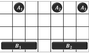
Figure 2: An example of the initial positions of the agents (A1, A2, A3) and blockers (B1, B2) in the blocker task.

Experiments

We evaluate the performance of Determinantal SARSA on the blocker task (Sallans and Hinton 2001; 2004; Heess, Sil-ver, and Teh 2013; Sallans 2002) and the stochastic policy task (Heess, Silver, and Teh 2013; Sallans 2002), which have been designed to evaluate the performance of multi-agent re-inforcement learning methods. The blocker task is on a fully observable environment, while the stochastic policy task in-volves partial observability. We compare the proposed ap-proach against the existing apap-proaches to multi-agent re-inforcement learning with non-factored action structures (i.e., taking into account the value of a team-action rather than the value of the individual action of an agent) (Sal-lans and Hinton 2001; 2004; Heess, Silver, and Teh 2013; Sallans 2002). We closely follow the instances considered in Heess, Silver, and Teh (2013) and compare our results against those reported in Heess, Silver, and Teh (2013). All of the experiments are carried out with Python implementa-tion on a workstaimplementa-tion having 48 GB memory and 4.0 GHz CPU.

Blocker Task

In the blocker task, we seek to control an agent-team (con-sisting of three agents) in a collaborative manner so that one of the agents reaches the end zone, while two block-ers hinder the agents. Figure 2 shows an example of the initial positions of the agents (A1, A2, A3) and the blockers (B1, B2). The field is a grid of four rows and seven columns. Each agent starts at uniformly random positions in the top row. Each blocker, who occupies three squares, starts at uni-formly random positions in the bottom row. The goal of the agent-team is to let one of the agents reach the end zone (bottom row) by avoiding the blockers.

At each step, each agent can move one step in one of the four directions or stay unmoved. After all of the agents take actions, each blocker moves one step to the right or to the left if doing so can block an agent; otherwise, the blocker stays unmoved. If one of the agents reaches the end zone, the agent-team receives+1reward for that step. Otherwise, the agent-team incurs−1reward per step. See Heess, Silver, and Teh (2013) for more details about the exact settings.

For this fully observable task, we learn to control the agents via Determinantal SARSA withDt ≡ I. Here, we

represent the team-actionatby a4×7 = 28dimensional

binary vectorx, where each dimension corresponds to one of the4×7squares constituting the grid. Specifically, the

Heess Silver Teh

N K prototypical actions

task 1 5 2 (0 0 1 0 1)

(0 1 0 1 1)

task 2 6 3 (1 1 0 0 0 0)

(0 0 1 1 0 0) (0 0 0 0 1 1)

task 3 8 3 (0 0 1 0 1 0 1 1)

(0 1 0 1 1 1 0 0)

(1 1 1 0 1 0 0 0) 0 10000 20000

0 2 4 6

Task 1

av. rew. / step

0 10000 20000

0 2 4

Task 2

# actions

0 10000 20000

0 2 4

Task 3

Figure 4.1: Stochastic policy task: The table shows the task-parameters for the three

ver-sions of the task. Results are shown for ENATDAC (green circles), EQNAC

(blue squares), SARSA (red crosses), and NN (magenta). Black lines show

av-erage reward for optimal policy; light gray lines show rewards with independent

actions.

Figure 4.2: Blocker task: The

top

plot illustrates several

steps in a blocker game (adapted from

Sallans

and Hinton 2004

). To win, the agents need to

cooperate. Here, agents 1,2 force the

block-ers to split so that agent 3 can enter the end

zone in the middle. The

bottom

plot shows, for

each algorithm, mean and standard deviation

of the average reward per step of the learned

policies for 20 restarts with diﬀerent random

initialziations (see Fig.

B.3 in the

supplemen-tal material for individual traces).

1 2

3

A

B

C

D

80000 240000 400000

−1 −0.9 −0.8 −0.7

# actions

avg. reward per action

SARSA NN EQNAC ENATDAC

transitions into state

k

+ 1

(or into state

1 from

K

). Otherwise the state is unchanged and

no reward is provided. Since the agent does not observe the environment state the optimal

policy is to choose the

K

“good” action conﬁgurations with equal probability, achieving an

average reward of

10 K

. A deterministic policy will get zero reward since it will get stuck in one

of the states. Further, it is necessary to model

dependencies

between action variables: for

independently drawn action variables the probability of generating a “good” conﬁguration

is very low. We consider three versions of the task with

N

= 5

,

6 ,

8 , and

K

= 2

,

3 ,

3 (cf.

Fig.

4.1 ). The ﬁrst version was considered in

Sallans

[

2002

]. We used an RBM with 1 hidden

unit for task 1 and 2 hidden units for tasks 2 and 3. Training was performed for 20000

ac-tions. Results are shown in Fig.

4.1 . The NN models each action dimension independently

and therefore performs very poorly (see supplemental material for further discussion). In

contrast, the RBM learns to represent these correlations via stochastic latent variables and

performs very eﬀectively. When training the RBM, ESARSA is only able to ﬁnd the optimal

policy for task 1, whereas EQNAC and ENATDAC ﬁnd optimal policies in all cases.

3

The

blocker task

(

Sallans 2002

;

Sallans and Hinton 2004

) is a multi-agent task in which

agents have to reach the end zone at the top of a playing ﬁeld while blockers try to stop

3. Although only the first 20000 actions are shown we allowed 50000 actions for ESARSA training. For

task 2 additional training leads to a small improvement relative to the performance after 20000 actions

but not for task 3 (see also Fig.

B.1 in supplemental material).

50

1

Figure 3: Performance of Determinantal SARSA (black curve) and baseline methods (colored curves) on the blocker task (the black curve is drawn on Figure 4.2 of Heess, Sil-ver, and Teh (2013)). Each curve shows the mean and the standard deviation, over 20 runs, of the average reward per action.

i-th dimension indicates whether an agent occupies thei-th square after taking the team-actionat((xt)i= 1) or not. We

use a full rank kernel (i.e.,28×28matrixV), which tends to perform best for this particular task. Also,αin (4) is omit-ted, becausext=0never appears in this task. In Boltzmann

exploration, we sample a team-action according to the exact distribution of 26 without the use of MCMC, because ex-act sampling is trex-actable for this task, where the number of feasible team-actions is at most53 _{= 125}_{and can be much} smaller in some states.

Figure 33 shows the average reward per step, for ev-ery 40,000 steps (and for evev-ery 4,000 steps during the ini-tial 40,000 steps of Determinantal SARSA), against the total number of steps for Determinantal SARSA (black) and baseline methods (colored) studied in Heess, Silver, and Teh (2013). The baselines are free-energy SARSA (SARSA), neural network (NN), energy-based Q-value nat-ural actor critic (EQNAC), and energy-based natnat-ural TD actor-critic (ENATDAC). We find that the average reward for Determinantal SARSA already exceeds−0.7during 20,000-24,000 steps, which is approximately 10 times faster than the baseline methods.

A potential weakness of Determinantal SARSA is rela-tively large standard deviation in the average reward. The average reward has stayed below−0.9for one of the 20 runs. This suggests that Determinantal SARSA may be trapped in poor local optima, depending on initial conditions, where the initial values ofVhave been chosen by adding noise to each element of the identity matrix, where the noise is uniformly at random between−0.01and0.01.

While learningL, Determinantal SARSA learns the

qual-3

Here, we let the learning rate decrease over time with a “simple back-off strategy” (Dabney and Barto 2012), where the learning rate at steptisηt = η0 min{1,104/(t+ 1)}withη0 = 10−3.

The discount factor is setρ= 0.9. In Boltzmann exploration, we let the inverse temperatureβtincrease over timet:βt= (β104)t/10

4

withβ104 = 10.0. These hyper-parameters are set as the values

that give best performance for the initial 10,000 steps of one run, where the candidate values areη0 ∈ {10−2,10−3,10−4},ρ ∈

(6)

1 2 3 4 5 6 7 1

2

3 0.2

0.4 0.6 0.8 1.0

(a) Learned quality

(1, 1) (1, 2) (1, 3) (1, 4) (1, 5) (1, 6) (1, 7) (2, 1) (2, 2) (2, 3) (2, 4) (2, 5) (2, 6) (2, 7) (3, 1) (3, 2) (3, 3) (3, 4) (3, 5) (3, 6) (3, 7) (1, 1)

(1, 2) (1, 3) (1, 4) (1, 5) (1, 6) (1, 7) (2, 1) (2, 2) (2, 3) (2, 4) (2, 5) (2, 6) (2, 7) (3, 1) (3, 2) (3, 3) (3, 4) (3, 5) (3, 6) (3, 7)

0.2 0.4 0.6 0.8 1.0

(b) Learned similarity

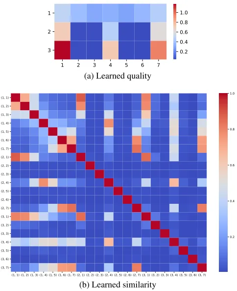
Figure 4: The quality of the positions (top) and the absolute value of their similarity (bottom) learned by Determinantal SARSA.

ity of each position and the similarity between those posi-tions. In fact, the learnedLcan be decomposed into qual-ity scoreq = diag(L)and similarity measures S, whose elements are Si,j = Li,j/pLi,iLj,j (see (85)-(86) from

Kulesza and Taskar (2012)).

Figure 4 shows the quality score and the similarity mea-sure learned by Determinantal SARSA. The figure of the quality score corresponds to the top three rows of the grid field in Figure 2. Three positions in the third row ((3, 1), (3, 4), (3, 7)) are found to have high value, as an agent might reach the end zone in the next step from those positions. Learning quality score is not sufficient, because then all of the agents can head toward the same position to be blocked by a defender. The similarity measure shows that the po-sitions that are close to each other (e.g., (2, 1) and (3, 1)) are found to have high similarity. This makes agents tend to move toward the positions that not only have high qual-ity but also are far away from each other, letting the three agents occupy (3, 1), (3, 4), and (3, 7), making it impossi-ble for the defenders to block all of the agents. Note that the agent-team has learned such quality and similarity only from the experiences of taking actions, observing states, and earning reward. In particular, no geographical information about the positions is given.

Stochastic Policy Task

Next, we study three stochastic policy tasks, where an agent-team iteratively chooses agent-team-actions from the space ofN

dimensional binary vectors, whereN = 5in Task 1,N = 6

in Task 2, andN= 8in Task 3. States are unobservable but can be represented as binary vectors ofNdimensions. When the team-action matches the state, the agent-team receives

+10reward, and the state transitions to another. Otherwise, the agent-team receives no reward, and the state stays un-changed. The state transitions in a deterministic and cyclic manner among two states in Task 1 and three states in Task 2-3.

In stochastic policy tasks, it is important to take into ac-count correlation between actions (bits): some pairs of bits should be selected together, and others should not. We use determinant to take into account ”diversity”, but it is non-trivial what ”diversity” really means here. Determinantal SARSA learns a feature vector for each bit in a way that the bits that should not be selected together have similar fea-ture vectors, and those that should be selected together have rather orthogonal feature vectors. We will see that this ”di-versity” helps in stochastic policy tasks.

We learn to control the agent-team via Determinantal SARSA. Here, the team-action at has the natural N-bit

feature vector xt, and we let the observation at time t to

be the previous team-action zt = xt−1. We then use full rank matrices (K = M = N), so that V and Dt are

N ×N. Throughout, we use a lag-1 autoregressive model

dt(φ) =b+W ztas our time-series model and set the

dis-count factor asρ= 0, because those settings are the simplest and generally perform well for stochastic policy tasks. In Boltzmann exploration, we run MCMC for 100 steps, start-ing from a uniformly random team-action (each bit is 1 with probability 0.5).

Figure 54 _{shows the average reward per step against the}

total number of steps. The black curves show the perfor-mance of Determinantal SARSA, and the colored curves show the performance of the four baseline methods studied in Heess, Silver, and Teh (2013). The color of each curve indicates the specific method, as is shown in the legend of Figure 3.

Overall, Determinantal SARSA performs substantially better than the baseline methods consistently for all of the three tasks, where the size of the action space is varied from

25_{= 32}_{(Task 1) to}₂8_{= 256}_{in (Task 3). In particular,} De-terminantal SARSA finds nearly optimal history-dependent policies within the steps that the best baseline method needs to find nearly optimal Markovian policies. The agent-team

4_{Here, the hyper parameters are set as the values that give best} performance for the initialn = 1,000iterations of one run for Task 1-2, but we letn= 10,000for Task 3, which requires longer iterations to observe meaningful difference. Specifically, the learn-ing rate is set asη0= 0.005for Task 1-2 andη0= 0.003for Task

(7)

Heess Silver Teh

N K prototypical actions

task 1 5 2 (0 0 1 0 1)

(0 1 0 1 1)

task 2 6 3 (1 1 0 0 0 0)

(0 0 1 1 0 0) (0 0 0 0 1 1)

task 3 8 3 (0 0 1 0 1 0 1 1)

(0 1 0 1 1 1 0 0)

(1 1 1 0 1 0 0 0) 0 10000 20000

0 2 4 6

Task 1

av. rew. / step

0 10000 20000

0 2 4

Task 2

# actions

0 10000 20000

0 2 4

Task 3

Figure 4.1: Stochastic policy task: The table shows the task-parameters for the three

ver-sions of the task. Results are shown for ENATDAC (green circles), EQNAC

(blue squares), SARSA (red crosses), and NN (magenta). Black lines show

av-erage reward for optimal policy; light gray lines show rewards with independent

actions.

Figure 4.2: Blocker task: The

top

plot illustrates several

steps in a blocker game (adapted from

Sallans

and Hinton 2004

). To win, the agents need to

cooperate. Here, agents 1,2 force the

block-ers to split so that agent 3 can enter the end

zone in the middle. The

bottom

plot shows, for

each algorithm, mean and standard deviation

of the average reward per step of the learned

policies for 20 restarts with diﬀerent random

initialziations (see Fig.

B.3 in the

supplemen-tal material for individual traces).

1 2

3

A

B

C

D

80000 240000 400000

−1 −0.9 −0.8 −0.7

# actions

transitions into state

k

+ 1

(or into state

1 from

K

). Otherwise the state is unchanged and

no reward is provided. Since the agent does not observe the environment state the optimal

policy is to choose the

K

“good” action conﬁgurations with equal probability, achieving an

average reward of

10 K

. A deterministic policy will get zero reward since it will get stuck in one

of the states. Further, it is necessary to model

dependencies

between action variables: for

independently drawn action variables the probability of generating a “good” conﬁguration

is very low. We consider three versions of the task with

N

= 5

,

6 ,

8 , and

K

= 2

,

3 ,

3 (cf.

Fig.

4.1 ). The ﬁrst version was considered in

Sallans

[

2002

]. We used an RBM with 1 hidden

unit for task 1 and 2 hidden units for tasks 2 and 3. Training was performed for 20000

ac-tions. Results are shown in Fig.

4.1 . The NN models each action dimension independently

and therefore performs very poorly (see supplemental material for further discussion). In

contrast, the RBM learns to represent these correlations via stochastic latent variables and

performs very eﬀectively. When training the RBM, ESARSA is only able to ﬁnd the optimal

policy for task 1, whereas EQNAC and ENATDAC ﬁnd optimal policies in all cases.

3 The

blocker task

(

Sallans 2002

;

Sallans and Hinton 2004

) is a multi-agent task in which

agents have to reach the end zone at the top of a playing ﬁeld while blockers try to stop

3. Although only the first 20000 actions are shown we allowed 50000 actions for ESARSA training. For

task 2 additional training leads to a small improvement relative to the performance after 20000 actions

but not for task 3 (see also Fig.

B.1 in supplemental material).

1

8 10

(a) Task 1

Heess Silver Teh

N K prototypical actions task 1 5 2 (0 0 1 0 1)

(0 1 0 1 1)

task 2 6 3 (1 1 0 0 0 0) (0 0 1 1 0 0) (0 0 0 0 1 1)

task 3 8 3 (0 0 1 0 1 0 1 1) (0 1 0 1 1 1 0 0)

(1 1 1 0 1 0 0 0) 0 10000 20000

0 2 4 6

Task 1

av. rew. / step

0 10000 20000

0 2 4

Task 2

# actions

0 10000 20000

0 2 4

Task 3

Figure 4.1: Stochastic policy task: The table shows the task-parameters for the three

ver-sions of the task. Results are shown for ENATDAC (green circles), EQNAC

(blue squares), SARSA (red crosses), and NN (magenta). Black lines show

av-erage reward for optimal policy; light gray lines show rewards with independent

actions.

Figure 4.2: Blocker task: The

top

plot illustrates several

steps in a blocker game (adapted from

Sallans

and Hinton 2004

). To win, the agents need to

cooperate.

Here, agents 1,2 force the

block-ers to split so that agent 3 can enter the end

zone in the middle. The

bottom

plot shows, for

each algorithm, mean and standard deviation

of the average reward per step of the learned

policies for 20 restarts with diﬀerent random

initialziations (see Fig.

B.3 in the

supplemen-tal material for individual traces).

1 2

3

A B

C D

80000 240000 400000 −1

−0.9 −0.8 −0.7

# actions

transitions into state

k

+ 1

(or into state

1 from

K

). Otherwise the state is unchanged and

no reward is provided. Since the agent does not observe the environment state the optimal

policy is to choose the

K

“good” action conﬁgurations with equal probability, achieving an

average reward of

10

K

. A deterministic policy will get zero reward since it will get stuck in one

of the states. Further, it is necessary to model

dependencies

between action variables: for

independently drawn action variables the probability of generating a “good” conﬁguration

is very low. We consider three versions of the task with

N

= 5

,

6 ,

8 , and

K

= 2

,

3 ,

3 (cf.

Fig.

4.1 ). The ﬁrst version was considered in

Sallans

[

2002

]. We used an RBM with 1 hidden

unit for task 1 and 2 hidden units for tasks 2 and 3. Training was performed for 20000

ac-tions. Results are shown in Fig.

4.1 . The NN models each action dimension independently

and therefore performs very poorly (see supplemental material for further discussion). In

contrast, the RBM learns to represent these correlations via stochastic latent variables and

performs very eﬀectively. When training the RBM, ESARSA is only able to ﬁnd the optimal

policy for task 1, whereas EQNAC and ENATDAC ﬁnd optimal policies in all cases.

3

The

blocker task

(

Sallans 2002

;

Sallans and Hinton 2004

) is a multi-agent task in which

agents have to reach the end zone at the top of a playing ﬁeld while blockers try to stop

3. Although only the first 20000 actions are shown we allowed 50000 actions for ESARSA training. For task 2 additional training leads to a small improvement relative to the performance after 20000 actions but not for task 3 (see also Fig. B.1 in supplemental material).

50

1

6 8 10

(b) Task 2

Heess Silver Teh

N K prototypical actions task 1 5 2 (0 0 1 0 1)

(0 1 0 1 1)

task 2 6 3 (1 1 0 0 0 0) (0 0 1 1 0 0) (0 0 0 0 1 1)

task 3 8 3 (0 0 1 0 1 0 1 1) (0 1 0 1 1 1 0 0)

(1 1 1 0 1 0 0 0) 0 10000 20000

0 2 4 6

Task 1

av. rew. / step

0 10000 20000

0 2 4

Task 2

# actions

0 10000 20000

0 2 4

Task 3

Figure 4.1: Stochastic policy task: The table shows the task-parameters for the three

ver-sions of the task. Results are shown for ENATDAC (green circles), EQNAC

(blue squares), SARSA (red crosses), and NN (magenta). Black lines show

av-erage reward for optimal policy; light gray lines show rewards with independent

actions.

Figure 4.2: Blocker task: The

top

plot illustrates several

steps in a blocker game (adapted from

Sallans

and Hinton 2004

). To win, the agents need to

cooperate.

Here, agents 1,2 force the

block-ers to split so that agent 3 can enter the end

zone in the middle. The

bottom

plot shows, for

each algorithm, mean and standard deviation

of the average reward per step of the learned

policies for 20 restarts with diﬀerent random

initialziations (see Fig.

B.3 in the

supplemen-tal material for individual traces).

1 2

3

A B

C D

80000 240000 400000 −1

−0.9 −0.8 −0.7

# actions

transitions into state

k

+ 1

(or into state

1 from

K

). Otherwise the state is unchanged and

no reward is provided. Since the agent does not observe the environment state the optimal

policy is to choose the

K

“good” action conﬁgurations with equal probability, achieving an

average reward of

10

K

. A deterministic policy will get zero reward since it will get stuck in one

of the states. Further, it is necessary to model

dependencies

between action variables: for

independently drawn action variables the probability of generating a “good” conﬁguration

is very low. We consider three versions of the task with

N

= 5

,

6 ,

8 , and

K

= 2

,

3 ,

3 (cf.

Fig.

4.1 ). The ﬁrst version was considered in

Sallans

[

2002

]. We used an RBM with 1 hidden

unit for task 1 and 2 hidden units for tasks 2 and 3. Training was performed for 20000

ac-tions. Results are shown in Fig.

4.1 . The NN models each action dimension independently

and therefore performs very poorly (see supplemental material for further discussion). In

contrast, the RBM learns to represent these correlations via stochastic latent variables and

performs very eﬀectively. When training the RBM, ESARSA is only able to ﬁnd the optimal

policy for task 1, whereas EQNAC and ENATDAC ﬁnd optimal policies in all cases.

3

The

blocker task

(

Sallans 2002

;

Sallans and Hinton 2004

) is a multi-agent task in which

agents have to reach the end zone at the top of a playing ﬁeld while blockers try to stop

3. Although only the first 20000 actions are shown we allowed 50000 actions for ESARSA training. For task 2 additional training leads to a small improvement relative to the performance after 20000 actions but not for task 3 (see also Fig. B.1 in supplemental material).

50

1

6 8 10

(c) Task 3

Figure 5: Performance of Determinantal SARSA (black curves) and baseline methods (colored curves) on the stochastic policy tasks (black curves are drawn on Figure 4.1 of Heess, Silver, and Teh (2013)). Each curve shows the mean and the standard deviation, over 20 runs, of the average reward per step (team-action) for every 2,000 steps (team-actions). Gray lines show the average reward per step for the random policy (The gray straight line for Task 1 was drawn at wrong values in Heess, Silver, and Teh (2013), which remains here.). Black straight lines show the average reward per step for the optimal Markovian policy or the optimal history-dependent policy.

obtains +10 reward every step with the optimal history-dependent policy, while the agent-team can obtain the re-ward with probability 1/|S| with the optimal Markovian policy, where|S|is the number of hidden states.

Conclusion

We have proposed the approach of using the determinant of a matrix in reinforcement learning. Determinant plays the role of taking into account diversity in team-actions. When the matrix is diagonal, our approach reduces to the standard ap-proach of factored action space, where multi-agents choose actions independently. Determinantal SARSA can deal with partial observability by using determinant with a time-series model, which can then be trained in an end-to-end man-ner. In our experiments, Determinantal SARSA substantially outperforms existing methods that have been proposed for dealing with high dimensional action space, which typically appears in multi-agent reinforcement learning.

The proposed Determinantal SARSA can effectively deal with exponentially large team-action space. When there are 2N _{possible team-actions, Determinantal SARSA has}

at most O(N3₎ _{computational complexity and can have} smaller complexity by assuming a low rank structure. Notice that learning a Q function with Determinantal SARSA does not need to deal with a partition function, which is the source of computational bottleneck in the case of learning DPPs. As a result, the most computationally expensive step of learning a Q function with Determinantal SARSA is in computing the pseudo inverse of aκ×KmatrixV(x), whereκis the num-ber of 1 inx(e.g., number of agents), andKis the rank of the kernel, and these can be much smaller thanN.

A DPP (or an annealed determinantal distribution) natu-rally appears with Determinantal SARSA when we choose team-actions according to the standard approach of Boltz-mann exploration. We can thus exploit existing techniques for sampling from DPPs to choose team-actions from a com-binatorially large space. However, the kernel Lt that we

learn with Determinantal SARSA may be used to sample actions according to other distributions that induce diversity. This leads to non-standard exploration strategies but possi-bly with reduced sampling cost. For example, the learned

Ltmay be used with Mat´ern’s hard-core processes (Mat´ern

1986; Haenggi 2012), where the actions are sampled in-dependently according to their relevance and thinned (re-moved) on the basis of their similarity.

A focus of our study has been on learning a time-varying kernelLtwith reinforcement learning. LearningLtmeans

learning what actions are relevant and what actions are sim-ilar to each other, where these relevance and simsim-ilarity can vary over time. We have demonstrated that one can learn those relevance and similarity only from observing states, taking team-actions, and getting rewards. In our framework, actions are considered to be similar to each other when a team-action consisting of those actions has lower value than what is expected from the individual relevance of those ac-tions.

Finally, SARSA is only one method of reinforcement learning, and the approach of using determinant to approxi-mate action-value functions or policies is largely applicable to other methods of reinforcement learning. Future work in-cludes using determinant with more sophisticated methods of reinforcement learning for practical tasks of multi-agent reinforce learning such as sports games.

Acknowledgments

This work was supported by JST CREST Grant Number JP-MJCR1304, Japan.

References

Baird, L. C. 1995. Residual algorithms: Reinforcement learning with function approximation. InProc. of the 12th International Conference on Machine Learning, 30–37. Belabbas, M.-A., and Wolfe, P. J. 2009. On landmark selec-tion and sampling in high-dimensional data analysis.

(8)

sophical Transactions of the Royal Society: Mathematical, Physical and Engineering Sciences367:4295–4312. Boyan, J. A., and Moore, A. W. 1995. Generalization in re-inforcement learning: Safely approximating the value func-tion. InAdvances in Neural Information Processing Systems 7. 369–376.

Dabney, W., and Barto, A. G. 2012. Adaptive step-size for online temporal difference learning. In Proc. of the 26th AAAI Conference on Artificial Intelligence, 872–878. Elfwing, S.; Uchibe, E.; and Doya, K. 2016. From free energy to expected energy: Improving energy-based value function approximation in reinforcement learning. Neural Networks84:17–27.

Foerster, J.; Nardelli, N.; Farquhar, G.; Afouras, T.; Torr, P.; Kohli, P.; and Whiteson, S. 2017. Stabilising experience replay for deep multi-agent reinforcement learning. InProc. of the 34th International Conference on Machine Learning, 1146–1155.

Gartrell, M.; Paquet, U.; and Koenigstein, N. 2017. Low-rank factorization of determinantal point processes. In

Proc. of the 31st AAAI Conference on Artificial Intelligence, 1912–1918.

Gillenwater, J. A.; Kulesza, A.; Fox, E.; and Taskar, B. 2014. Expectation-maximization for learning determinantal point processes. InAdvances in Neural Information Processing Systems 27. 3149–3157.

Gillenwater, J. 2014. Approximate Inference for Determi-nantal Point Processes. Ph.D. Dissertation.

Gong, B.; Chao, W.-L.; Grauman, K.; and Sha, F. 2014. Di-verse sequential subset selection for supervised video sum-marization. InAdvances in Neural Information Processing Systems 27. 2069–2077.

Gupta, J. K.; Egorov, M.; and Kochenderfer, M. 2017. Coop-erative multi-agent control using deep reinforcement learn-ing. InProc. of the International Conference on Autonomous Agents and Multiagent Systems, 66–83.

Haenggi, M. 2012. Stochastic Geometry for Wireless Net-works. Cambridge University Press.

Hausknecht, M., and Stone, P. 2015. Deep recurrent Q-learning for partially observable MDPs. InSequential De-cision Making for Intelligent Agents: Papers from the AAAI 2015 Fall Symposium. 29–37.

Heess, N.; Silver, D.; and Teh, Y. W. 2013. Actor-critic reinforcement learning with energy-based policies. InProc. of the 10th European Workshop on Reinforcement Learning, volume 24, 45–58.

Kang, B. 2013. Fast determinantal point process sampling with application to clustering. InAdvances in Neural Infor-mation Processing Systems 26. 2319–2327.

Kathuria, T.; Deshpande, A.; and Kohli, P. 2016. Batched gaussian process bandit optimization via determinantal point processes. InAdvances in Neural Information Processing Systems 29. 4206–4214.

Kulesza, A., and Taskar, B. 2011. k-DPPs: Fixed-size deter-minantal point processes. InProc. of the 28th International Conference on Machine Learning, 1193–1200.

Kulesza, A., and Taskar, B. 2012.Determinantal Point Pro-cesses for Machine Learning. Hanover, MA, USA: Now Publishers Inc.

Macchi, O. 1975. The coincidence approach to stochastic point processes. Advances in Applied Probability7:83–122. Maei, H. R., and Sutton, R. S. 2010. GQ (λ): A general gradient algorithm for temporal-difference prediction learn-ing with eligibility traces. InProc. of the 3rd Conference on Artificial General Intelligence, 91–96.

Maei, H. R.; Szepesv´ari, C.; Bhatnagar, S.; Precup, D.; Sil-ver, D.; and Sutton, R. S. 2009. Convergent temporal-difference learning with arbitrary smooth function approxi-mation. InAdvances in Neural Information Processing Sys-tems 22. 1204–1212.

Mariet, Z., and Sra, S. 2016. Kronecker determinantal point processes. InAdvances in Neural Information Processing Systems 29. 2694–2702.

Mat´ern, B. 1986.Spatial Variation. Lecture Notes in Statis-tics. Springer, 2nd edition.

Osogami, T., and Otsuka, M. 2015. Seven neurons mem-orizing sequences of alphabetical images via spike-timing dependent plasticity.Scientific Reports5:14149.

Osogami, T.; Raymond, R.; Goel, A.; Shirai, T.; and Mae-hara, T. 2018. Dynamic determinantal point processes. In

Proc. of the 32nd AAAI Conference on Artificial Intelligence, 3868–3875.

Osogami, T. 2017. Boltzmann machines for time-series. Technical Report RT0980, IBM Research - Tokyo.

Qiao, M.; Xu, R. Y. D.; Bian, W.; and Tao, D. 2016. Fast sampling for time-varying determinantal point pro-cess.ACM Transactions on Knowledge Discovery from Data

11(Article No. 8).

Sallans, B., and Hinton, G. E. 2001. Using free energies to represent Q-values in a multiagent reinforcement learning task. InAdvances in Neural Information Processing Systems 13. 1075–1081.

Sallans, B., and Hinton, G. E. 2004. Reinforcement learning with factored states and actions.Journal of Machine Learn-ing Research5:1063–1088.

Sallans, B. 2002. Reinforcement learning for factored Markov decision processes. Ph.D. Dissertation.

Snoek, J.; Zemel, R.; and Adams, R. P. 2013. A deter-minantal point process latent variable model for inhibition in neural spiking data. InAdvances in Neural Information Processing Systems 26. 1932–1940.

Wachinger, C., and Golland, P. 2015. Sampling from deter-minantal point processes for scalable manifold learning. In

Proc. of the International Conference on Information Pro-cessing in Medical Imaging, 687–698.