The Thirty-Third AAAI Conference on Artificial Intelligence (AAAI-19)
Partially Observable Multi-Sensor Sequential Change
Detection: A Combinatorial Multi-Armed Bandit Approach
Chen Zhang
Department of Industrial Engineering Tsinghua University
Beijing, China, 100084 [email protected]
Steven C.H. Hoi
School of Information Systems Singapore Management UniversitySingapore 178902 [email protected]
Abstract
This paper explores machine learning to address a problem of Partially Observable Multi-sensor Sequential Change Detec-tion (POMSCD), where only a subset of sensors can be ob-served to monitor a target system for change-point detection at each online learning round. In contrast to traditional Multi-sensor Sequential Change Detection tasks where all the sen-sors are observable, POMSCD is much more challenging be-cause the learner not only needs to detect on-the-fly whether a change occurs based on partially observed multi-sensor data streams, but also needs to cleverly choose a subset of informa-tive sensors to be observed in the next learning round, in order to maximize the overall sequential change detection perfor-mance. In this paper, we present the first online learning study to tackle POMSCD in a systemic and rigorous way. Our ap-proach has twofold novelties: (i) we attempt to detect change-points from partial observations effectively by exploiting po-tential correlations between sensors, and (ii) we formulate the sensor subset selection task as a Multi-Armed Bandit (MAB) problem and develop an effective adaptive sampling strategy using MAB algorithms. We offer theoretical analysis for the proposed online learning solution, and further validate its em-pirical performance via an extensive set of numerical studies together with a case study on real-world data sets.
Introduction
Unsupervised learning for sequential monitoring of com-plex systems (a.k.a., sequential change detection) is ubiqui-tous in a wide range of applications, such as quality control in manufacturing processes, logistic systems, transportation networks, electrical grids, the internet of things (IoT) sys-tems, etc. Typically, to capture information about the un-derlying system state in real time, a massive array of vari-ables are measured continuously and sequentially for prompt change detection and timely decision making. However, in practice, the acquisition of continuously measurements of such a large amount of variables may be infeasible due to resource constraints. For example, the number of available sensors may be less than the number of interested variables to be monitored due to expensive cost of the sensors; or at each sensing epoch only a limited number of sensors can be set in the “ON” mode for measurement due to limited battery
Copyright c2019, Association for the Advancement of Artificial Intelligence (www.aaai.org). All rights reserved.
lifetime. Furthermore, when the number of variables is large and their measurement streams are generated in high veloc-ity, real-time analysis may be significantly hindered due to the constraints of system memory, storage space, transmis-sion bandwidth, computational power and processing speed. Consequently, in many applications, even if all variables can be measured, only partial observations of them can be trans-mitted back to the data fusion center for real-time analytics. All the above constraints trigger the demand of new learn-ing techniques to address the emerglearn-ing challenge of Par-tially Observable Multi-sensor Sequential Change Detection (POMSCD), where only a subset of sensors can be observed at each epoch for change detection. Specifically, consider a system characterized by a set ofpvariables (for example, in a manufacturing system, each variable corresponds to a fabrication characteristic). Signals of these variables at each sensing epochtare denoted asX(t) = [X1(t), . . . , Xp(t)], where each valueXi(t), i= 1, . . . , pis a scalar indicating the state of theithsystem characteristic at the current epoch
Related Work
Our work is related to the family of sequential change-point detection works, which has been extensively studied in the literature of statistics, machine learning and beyond (Xie and Siegmund 2013; Tartakovsky, Nikiforov, and Basseville 2014; Chan 2017; Aminikhanghahi and Cook 2017). How-ever, most existing studies assume all the variables with the target system can be fully observable, which are not di-rectly applicable to POMSCD in the partially observable context. To the best of our knowledge, the only closely re-lated works that attempt to address partial observations for multi-sensor change detection are Liu, Mei, and Shi (2015) and Xian, Wang, and Liu (2017). However, these two meth-ods are traditional statistics-based approaches, and do not exploit variables’ correlations. More critically, their detec-tion powers are not satisfactory in some cases (which will be demonstrated in numerical studies) due to their heuris-tic adaptive sensor allocation strategies which are based on the rule of thumb and cannot give theoretical guarantee. By contrast, we propose the first online learning scheme for POMSCD with rigorous theoretical guarantee, which care-fully exploits the correlation of variables and dynamically chooses the subset of informative sensors to maximize the detection power.
Our problem is also different from adaptive resource al-location problems such as ranking and selection (Nelson et al. 2001), statistical adaptive monitoring (Tartakovsky et al. 2006), multi-armed bandit (MAB)(Gai, Krishnamachari, and Jain 2010; Even-Dar, Mannor, and Mansour 2006; Bubeck, Wang, and Viswanathan 2013), active learning (Kapoor et al. 2007) and online feature selection (Wang et al. 2014), from the following perspectives: (i) In our prob-lem, change patterns can be any mean shift and are unknown in advance; hence, unsupervised learning is more suitable. However, most of current change detection methods via ac-tive learning or feature selection are based on supervised learning, assuming abnormal patterns can be known be-forehand for model training; (ii) We aim at a system-level change detection. When a change occurs, we aim to mini-mize the detection delay, while ranking and selection or tra-ditional MAB studies aim at identifying which variable is changed (Zhuang, Wang, and Wang 2017), i.e., detection in the variable level. Consequently, they may not guarantee an effective system-level performance; (iii) We allow different variables to have correlations with each other, and such cor-relation information can help for efficient detection. How-ever, most existing works across the above often assume the data streams are independent with each other.
Problem Formulation
Consider a system withpcorrelated variables, denote their signals at sensing epoch t as X(t) = [X1(t), . . . , Xp(t)]. Initially,X(t)independently and identically (i.i.d) follows a joint distribution p(X(t)|µ)with the mean vectorµ. At some unknown time epochτ, an unusual event (a change) occurs and affects an unknown subset of thepdata streams in the sense that if variableiis affected, the mean of its local observationsXi(t)changes fromµitoµcifor epocht≥τ.
The problem is to raise an alarm as quickly as possible af-ter the change occurs. This mean (location) shift is a popu-lar change pattern considered in many works, especially for statistical process control in manufacturing (Montgomery 2009). Without loss of generality, we set the before-change mean vector asµ=0when the system is in the normal con-dition, and set the post-change mean vector asµc6=0. Due to limited sensing resources, at each sensing epoch, we can only observemout ofpvariables(m≤p). By introducing the binary decision variablezitfor each variableXi(t)such thatzit = 1if and only ifXi(t)is observed at epocht, the sensing constraint can be expressed as Ppi=1zit = m,∀t. We denote by Z(t)the vector of indices corresponding to the selected variables/sensors for observations inX(t).
A general detection scheme to decide whether a change occurs is defined as a scheme of stopping timeT associated with a test statisticΛ(t),∀t. Typically, one can defineT = inft{Λ(t)> h}wherehis a pre-defined constant threshold. The interpretation of T is that, when T = n, the scheme stops at epochnand declares that a change has occurred in some variables somewhere in the first ntime epochs. We want the scheme to stop as soon as possible after a change occurs (in the abnormal condition) but will continue moni-toring without raising false alarms as long as possible if no change occurs (in the normal condition). In other words, we wantP(Λ(t) > h)as small as possible in the normal case and as large as possible in the abnormal case. The perfor-mance of a schemeT can be evaluated by two performance indicators: the Average Run Length (ARL) before a false alarm occurs in the normal case, i.e.,ARL0=E(T|τ=∞)
and the Average Detection Delay (ADD) in the abnormal case, i.e., ADDτ = E(T −τ|T > τ, τ < ∞). In prac-tice, the problem can be equivalently formulated as finding a change detection schemeT that minimizes the ADD per-formance subject to a constraint imposed on theARL0, i.e.,
ARL0must be greater than a predefined constant that
essen-tially controls the global false alarm rate.
Our Method
Consider a general change detection scheme for POMSCD, at each epocht, it first determines if the system is still in normal condition. If no, an alarm is triggered; otherwise, it determines the sampling strategy i.e.,Z(t+ 1)to choose a subset of sensors to observe at the next epocht+1within the sensing constraint. In particular, we address the following two issues: (1) how to construct a change detection scheme for the partially observed data streams with consideration of their correlations; and (2) how to learn a good strategy to determine whichmout of thepvariables to be sampled at each epoch to increase the detection power of the scheme.
Online Weighted Bayesian Change Detection
Assume up to the current epochn, no change alarm is trig-gered. Then based onZ(t), t = 1, . . . , n, we can estimate the current system state, i.e., the mean vector µ of thep
potential system changes than the past epochs, we would like to stress more effort on the current epochs in the estimation. As such, we enforce time decayed weightswn
t, t= 1, . . . , n on thensamples, in the sense thatwn
1 < wn2 < . . . < wnn, and get the weighted posterior distribution ofµis
˜
p(µ|XZ(1), . . . ,XZ(n))∝p0(µ)
n Y
t=1
p(XZ(t)|µ)w
n t, (1)
whereXZ(t) is the vector of observed variables of X(t),
andp0(µ)is the prior distribution. In this paper, we use the
exponential decaying weight, i.e.,wn
t = (1−λ)n−twith a small positive valueλ∈(0,0.1]. Then (1) can be written in an incremental way as
˜
p(µ|XZ(1), . . . ,XZ(n)) = (2) ˜
p(µ|XZ(1), . . . ,XZ(n−1))1−λp(XZ(n)|µ).
Following many previous works(Xie and Siegmund 2013; Liu, Mei, and Shi 2015), in this paper we assume X(t)
follows a Gaussian distribution with covariance matrix Σ. Though there also exist some works that consider more gen-eral distributions, all the current works are constructed in a FULLY observed context, and cannot be applied in our case. Since our main contribution is change detection with ADAP-TIVE SENSOR ALLOCATION for PARTIAL OBSERVED DATA STREAM, we focus on the most classical setting and would extend to more complex scenarios in future. In partic-ular, by settingp0(u)to be non-informative, (2) also follows
a Gaussian distribution with meanµnand covariance matrix
Vnwhich can be calculated incrementally as:
Vn−1= (1−λ)V−
1
n−1+E 0
Z(n)Σ −1
Z(n)EZ(n), (3)
µn=Vn[(1−λ)µn−1+E0Z(n)Σ −1
Z(n)XZ(n)].
HereΣZ(t)is theZ(t)rows and columns ofΣ, andEZ(t)∈
Rm×p. Itsithrow is a unit vector who has1at the position of theithelement inZ(t)and0otherwise.
Note thatµn of (3) is estimated by considering the cor-relation of different variables. For each variable i, its esti-matedµniis not only based on the past observations of it-selfXi(t), t= 1, . . . , n, but also on past observations of the other variablesXj(t), j 6=i, t = 1, . . . , n. In other words, even if variableiis not observed at epochn, its meanµni will still be updated according to its correlations with the other observed variables at epochn.
Based on (3), we can get the 1 −α confidence region of the current system mean vector µ as Cα = {u|(u−
µn)0V−1
n (u−µn)≤χ2p,1−α}, whereχ2p,1−αis the1−α upper critical value ofχ2pdistribution withpdegree of free-dom. Then if0∈ Cα, it means that we can not rejectµ6= 0
with1−αconfidence, andvice versa. As such, we can con-struct the test statistic as
Λ(n) = (0−µn)0V−n1(0−µn) =µ0nV−n1µn. (4) Now we evaluate some theoretical properties of (4) in both normal and abnormal conditions.
Lemma 1 When the system is still in the normal condition withµ =0, asλ → 0,Λ(n)asymptotically follows aχ2
p distribution withpdegree of freedom.
Based on Lemma 1, we can set a detection thresholdhfor
Λ(n) according to a pre-specific confidence levelα(false alarm rate), and define that if Λ(n) > h, the test statistic triggers an abnormal alarm.
Lemma 2 When the system goes to an abnormal condition withµ =µc since the first epoch withτ = 1, asλ → 0,
Λ(n)asymptotically follows a non-central chi-square distri-butionχ2
p(cn)with the non-centrality
cn=µ0cV−
1
n µc= n X
t=1
wtnµ0cZ(t)Σ −1
Z(t)µcZ(t).
Lemma 2 shows that the detection power ofΛ(n)is related to the non-centralitycn. A highercnindicates a larger detec-tion power. Furthermore,cndepends onVn, which is further related toZ(t), t= 1, . . . , n. As such, it is desirable to con-struct an adaptive sampling strategy to maximizecn.
Adaptive Sampling for Sensors Selection by
Combinatorial Multi-armed Bandit
The problem of choosing a subset Z with|Z| = m from
p variables at each sensing epoch n is similar to MAB with multiple plays (Gai, Krishnamachari, and Jain 2010; Komiyama, Honda, and Nakagawa 2015; Xia et al. 2016; Zhou and Tomlin 2018). However, we note that in our prob-lemcn cannot be decomposed as a combination ofm sep-arate functions ofµci, i ∈ Z(t), i.e., not a linear function of themselected variables. By contrast, different variables have cross-influence on each other via the precision matrix
ΦZ(t)=Σ− 1
Z(t). Furthermore, the cross-influence magnitude
between two selected variables, sayiandj, is further depen-dent on the other selected variablesz∈Z(t), z6=i, j, since
(ΦZ1)ij 6= (ΦZ2)ij if two setsZ1 6= Z2. This means that
we cannot simply select thesemvariables one by one. Instead, we propose to re-formulate the problem as a Combinatorial Multi-armed Bandit (CMAB) task, where we treat a setZas asuper arm, withM = mpsuper arms in total, and our goal is to select the best super arm. Specifi-cally, we define the set of all super arms asZ ={Zk, k =
1, . . . , M}. The reward of choosingZkat epochtis
rk(µc) =µcZ0 kΦZkµcZk =
X
i∈Zk
X
j∈Zk
φijZkµciµcj, (5)
whereφijZk is the(i, j)component ofΦZk. We are
inter-ested in designing a sampling strategy for this CMAB prob-lem that performs well with respect totime decayed expected regret, which is defined as
Rπn(µc) =
n X
t=1
wtnr?−Eπ( n X
t=1
wntrπ(t)(µc)), (6)
where r? = µ0
cZ?ΦZ?µcZ? is the reward of the optimal
super arms. Here Z? denote optimal arms, which are not necessarily unique. In particular, denote the true changed variable set of the p variables as Za, with the cardinal-ity |Za| = a. If a ≤ m, the optimal super arms Z?
Z?= arg maxZ⊂Za,|Z|=mµ0cZΦZµcZ. In other words, the
optimal sampling strategy is to select all the changed arms
i ∈Za (ifa ≤m) or select the best subset of the changed arms (ifa > m).
Though CMAB has attracted increasing attention re-cently, most of existing works focus on linear reward func-tions(Gai, Krishnamachari, and Jain 2010; Durand and Gagn´e 2014). However, as mentioned earlier, our reward function rk(µc) is nonlinear with the individual arms
µci, i ∈ Zk. So far to our best knowledge, the only related work for CMAB with non-linear reward functions is Chen et al. (2016). However, this work has additional assump-tions that the reward funcassump-tions of super arms should have the monotonicity property:the expected reward of playing any super armZ ∈ Zis monotonically nondecreasing with respect to their expectation vector, i.e., if for alli= 1, . . . , p,
µci ≤ µ0ci, we haverZ(µc)≤ rZ(µ0c),∀Z ∈ Z. Clearly, this cannot be satisfied in our case. Consequently, direct ap-plying these sampling strategies in the literature to our case would lose their regret bound and lead to poor detection power. As such, in this paper we develop a new CMAB strat-egy tailored for our reward function, based on the UCB al-gorithm. In particular, for each variable i at epoch n, the
1−2InvNorm(√γn)confidence interval of its mean µi is
µni−
√
γnvni, µni+
√
γnvni
, wherevni is thei diago-nal item of Vn representing the variance of the posterior distribution ofµi. Then the upper confidence bound of the estimated reward of choosingZkat epochtbased onµnis
X i∈Zk
X j∈Zk
φijZk
µni+sgn(φijZkµniµnj)sgn(µni)
√
γnvni
(7)
×µnj+sgn(φijZkµniµnj)sgn(µnj)
√
γnvnj
= X
i∈Zk
X j∈Zk
φijZkµniµnj+
q
γnφ2ijZkµ2nivnj
+
q
γnφ2ijZ
kµ
2
njvin+γn q
φ2
ijZkvnivnj,
where sgn(x) = 1,∀x ≥ 0 and sgn(x) = −1,∀x < 0. The first part of (7) emphasizes on exploitation of the best super arm so far we estimate, while the last three parts of (7) emphasize on exploration of other potential super arms by considering the estimation uncertainty. The termγn bal-ances exploitation and exploration. The bigger it gets, the more it favours arms with highvni(exploration). Ifγn = 0, the algorithm is greedy. In our algorithm, we set γn as
exp(γn) = 2(1−(1−λ)n)/λ. Then we can select the supper armZkthat maximizes (7) as the variable set to be sampled for epochn+ 1. The detailed adaptive sampling strategy is shown in Algorithm 1.
Theorem 1 By settingγn = 2 log(1−(1−λ)
n
λ2 ), theR
π n(µc) of Algorithm 1 is at most
h
2 max
Zl
4 ˜µ0Zl
˜
ΦZlI+ 2||Φ˜Zl||1
∆Zl
q
log(1−(1−λ)
n
λ2 )+
2m(1−(1−λ)n)ip∆max,
Algorithm 1:CMAB for adaptively samplingZt Input:Data streamsXn, n= 1, . . .,
initializevm, m= 1, . . . , M forn= 1, . . . ,dp/medo
Observe anymvariables that have not been observed so far.
Updateµ(n)andVnaccording to (3). forn=dp/me+ 1, . . .do
SelectZ ∈ ZforZ(n+ 1)by maximizing
X
i∈Z X
j∈Z
φijZµniµnj+ q
γnφ2ijZµ2nivnj (8)
+
q
γnφ2ijZµ2njvni+γn q
φ2
ijZvnivnj.
where µ˜Z(t) ∈ Rm×1 with elements {|µ
cj|}j∈Z(t);
˜
ΦZ(t) ∈ Rm×m with elements {|φij|}i,j∈Z(t);
∆Zl = µ
0
cZ?ΦZ?µcZ? − µ0cZ
lΦZlµcZl; q = 1 if
maxZl
4 ˜µ0ZlΦ˜ZlI+2||Φ˜Zl||1
∆Zl ≤1whileq= 2otherwise. Proof 1 To derive and bound the decayed expected regret of Algorithm 1, we can analyze the expected number of times that each non-optimal super arm is played, and sum this ex-pectation over all non-optimal super arms. In particular, we have
Rπn=Eπ[
n X t=1
wntr?−
n X t=1
wtnrπ(t)(µc))]≤∆max
X l∈Z
E[Tl(n)],
whereTl(n)means the weighted number of epochs thatZl is chosen from epoch 1 up to epochn.
We introduce {T˜j(n)}, j = 1, . . . , p, n = 1, . . . as a counter after the initialization period. It is updated in the following way: At each time epoch after the initialization period, one of the two cases must happen: (1) an optimal super arm is played; (2) a non-optimal super arm is played. In the first case, setT˜j(n) = ˜Tj(n−1),∀j= 1, . . . , p,and
˜
Tj(t) = ˜Tj(t)·(1−λ),∀j = 1, . . . , p, t = 1, . . . , n−1. When a non-optimal super armZk is picked at timen, be-sides updatingTj(n)by the same way as the first case, we choosej0 ∈ Zk such thatj0 = arg minj∈ZkTj(n−1). If
there are multiple such arms, we arbitrarily pick one, say
j0, and increaseT
j0(n)by 1. In this way, each time a
non-optimal arm is picked, exactly one element inT˜j(n)is incre-mented by 1. This implies that the total “weighted” number we have played the non-optimal super arms up to epochn
is equal to the sum of all counters in{T˜j(n)}1:p. Therefore, we have
X
l∈Z
E[Tl(n)] = p X
j=1
E[ ˜Tj(n)].
˜
Tj(n)is added by one at timen. Letdbe an arbitrary posi-tive integer. Then
˜
Tj(n) =
n X t=1
wtn{I˜j(t)} ≤d+
n X t=2
wtn{I˜j(t),T˜j(t−1)≥d}. (9)
WhenI˜j(t) = 1, a non-optimal super armZ(t)is picked from which armj = arg minj∈Z(t)T˜j(t−1)is selected to update. Then we have
˜
Tj(n)≤d+
n X t=2
wnt{
X i∈Z?
X j∈Z?
φ?ijµˆtiµˆtj+ q
γtφ?ij2µˆ2tivtj
+
q
γtφ?ji2µˆ2tjvti+γt q
φ?2
ijvtivtj
≤ X
i∈Z(t) X j∈Z(t)
φijZ(t)µˆtiµˆtj+
q
γtφ2ijZ(t)µˆ2tivtj
+
q
γtφ2jiZ(t)µˆ2tjvti+γt q
φ2
ijZ(t)vtivtj,T˜j(t−1)≥d}.
Note thatd≤T˜j(t−1) = minj∈Z(t)T˜j(t−1), this indicates
Tj(t)≥d,∀j ∈Z(t). The second part of (9) indicates that at least one of the following must be true:
X i∈Z?
X j∈Z?
φ?ijµˆtiµˆtj≤ X i∈Z?
X j∈Z?
φ?ijµciµcj−
q
γtφ?ij2µˆ2tivtj
(10)
−
q
γtφ?ji2µˆ2tjvti−γt q
φ?2
ijvtivtj;
X i∈Z(t)
X j∈Z(t)
φijZ(t)µˆtiµˆtj≥
X i∈Z(t)
X j∈Z(t)
φijZ(t)µciµcj (11)
+qγtφ2ijZ(t)µˆ2tivtj+ q
γtφ2jiZ(t)µˆ2tjvti+γt q
φ2
ijZ(t)vtivtj;
X i∈Z?
X j∈Z?
φ?ijµciµcj≤
X i∈Z(t)
X j∈Z(t)
φijZ(t)µciµcj (12)
+ 2qγtφ2ijZ(t)µˆ2tivtj+ 2 q
γtφ2jiZ(t)µˆ2tjvti+ 2γt q
φ2
ijZ(t)vtivtj.
Now we first find the probability upper bound for (10). In particular,
P[(10)]≤ X
i∈Z?
P[µci−µˆti≥
√
γtvti]≤
X i∈Z?
exp(−γtvti
2vti
),
by setting γn = 2 log(
1−(1−λ)n
λ2 ), we have P[(10)] ≤
mλ2 1−(1−λ)t.
Similarly, we can also getP[(11)]≤ mλ2
1−(1−λ)t.
Now we derive the upper bound of (12).
P[(12)] =P
∆Z(t)≤
X i∈Z(t)
X j∈Z(t)
2qγtφ2ijZ(t)µˆ2tivtj
+2qγtφ2jiZ(t)µˆ2tjvti+ 2γt q
φ2
ijZ(t)vtivtj i
≤P
∆Z(t)≤4 ˜µZ0(t)ΦZ˜ (t)I r
γt
d + 2||
˜
ΦZ(t)||1
γt
d
.
Ifd≥γt, we have
p[(12)]≤P
∆Z(t)≤(4 ˜µ0Z(t)Φ˜Z(t)I+ 2||Φ˜Z(t)||1) r
γt
d
.
This means that as long as we set d ≥
maxZl
4 ˜µ0ZlΦ˜ZlI+2||Φ˜
Zl||1 ∆Zl
2
γt the condition of (12)
is false. Ifd < γt, we have
p[(12)]≤Ph∆Z(t)≤(4 ˜µ0Z(t)Φ˜Z(t)I+ 2||Φ˜Z(t)||1)
γt
d
i
This means that as long as we set d ≥
maxZl
4 ˜µ0ZlΦ˜ZlI+2||Φ˜Zl||1 ∆Zl
γt the condition of (12)
is false.
E[ ˜Tj(n)]≤2 max
Zl
4 ˜µ0Z
l
˜
ΦZlI+ 2||ΦZ˜ l||1
∆Zl
!q
log(1−(1−λ)
n
λ2 )
+ 2m
n X t=1
λ2
1−(1−λ)t(1−λ) n−t
≤2 max
Zl
4 ˜µ0
Zl
˜
ΦZlI+ 2||Φ˜Zl||1
∆Zl
!q
log(1−(1−λ)
n
λ2 )
+ 2m(1−(1−λ)n),
whereq = 1ifmaxZl
4 ˜µ0ZlΦ˜ZlI+2||Φ˜
Zl||1
∆Zl ≤ 1andq = 2
otherwise. Consequently, we can conclude Theorem 1.
Corollary 1 Asn→ ∞,1−(1−λ)n →1, which is fixed. Then we haveRπ
n(µc)is asymptotically bounded by
R∞=
"
4 max
Zl
4 ˜µ0Z
l
˜
ΦZlI+ 2||ΦZ˜
l||1
∆Zl
!q
log(1
λ) + 2m
#
p∆max.
With Corollary 1, we can bound the asymptotic expected detection power ofΛ(n).
Corollary 2 Whenλ → 0 andτ = 1, the asymptotic ex-pected detection power of Λ(n)as n → ∞ based on the adaptive sampling strategy in Algorithm 1 is bigger than
1−Qp
2(
p
c?−R
∞,
√
h),
where c? = µ0
cZ?ΦZ?µcZ?, andQp/2 is the Marcum
Q-function.
The whole proposed change detection scheme is as fol-lows. For each new online sample X(n), we first observe its valuesXZ(n) and getΛ(n)according to (3) and (4). If Λ(n) > h, the scheme triggers an abnormal alarm and the system stops for diagnosis. Otherwise, the scheme decides
Z(n+ 1)by Algorithm 1.
Remark 1 Whenmorpis big, searching all theM = mp super arms might be time consuming, and the algorithm might be impractical for very large-scale problems with limited data processing resource. Therefore a more time-efficient algorithm is desirable. Recall that it isΦZ(t) that
makes cn a nonlinear function of the selected variables. If we force ΦZ(t) to be a diagonal matrix, we can
re-move all the cross-influence and makecn as the simplified
˜ cn =
Pn t=1
P i∈Z(t)µ
2
ci, which is a linear (and monotone) function of the square of each arm’s reward,µ2
ci. In this case, samplingZbased on (8) in Algorithm 1 is degenerated to the following strategy: calculating
ri=|µni|+
√
ranking ri from the largest to smallest asr(1) ≥ r(2) ≥
. . . ≥ r(p), and selecting the variables withr(1), . . . , r(m)
asZ(n+ 1). The selection by (13) is similar to the CMAB strategy in Chen et al. (2016).
In the following experiments, we denote the proposed de-tection scheme for POMSCD using the CMAB algorithm in Algorithm 1 with strategy (8) as “CMAB”, and the detection scheme for POMSCD using the simplified CMAB strategy in (13) as “CMAB(s)” for short.
Numerical Studies
We conduct extensive experiments on both synthetic and real-world data sets, to evaluate the performance of the pro-posed POMSCD detection schemes with the two CMAB strategies, i.e., “CMAB” and “CMAB(s)”. We compare our schemes with the following existing baselines:
• TRAS: the top-r adaptive sampling detection algorithm in Liu, Mei, and Shi (2015);
• NAS: the nonparametric anti-rank adaptive sampling al-gorithm in Xian, Wang, and Liu (2017);
In addition, we also include two additional variants of our detection scheme as follows:
• RAND: a variant of the proposed POMSCD scheme by replacing the adaptive sampling strategies (CMAB or CMAB(s)) with arandomstrategy, i.e.,Z(n+1)is drawn by randomly samplingmfrom a total ofpvariables;
• ORACLE: the proposed detection scheme for POMSCD but assuming all the pvariables arefully observable at each epoch. Clearly, this is just an oracle scheme and used as a performance upper bound of our detection scheme.
Synthetic Data Experiments
Our experiments considers two settings, p = 10 and
p = 100 respectively. For both settings, we set (Σ)ij =
0.5,∀i 6= j,m = 5 andλ = 0.1, and consider the fol-lowing two change patterns: (i) The first q variables have the same mean shift magnitude with the same sign, i.e.,
µc = [1, . . . ,1
| {z } q
,0, . . . ,0]×δ; (ii) The firstqvariables have
the same mean shift magnitude with opposite signs, i.e.,
µc = [1,−1,1, . . . ,1,−1
| {z }
q
,0, . . . ,0]×δ; where δ is the
shift magnitude. We set q = 4 for p = 10and q = 16
forp = 100. For each algorithm, we set itshsuch that its
ARL0 = 200, and we evaluate its detection performance
in terms of ADD50 with τ = 50. All the ADDs in
sub-sequent simulations are calculated based on10000 simula-tion replicasimula-tions. For TRAS, we set its parameterr = m,
µmin = 0.25 and∆ = 0.03 for both settings according to the recommendation of Liu, Mei, and Shi (2015). For NAS, we set its parameter k = 0.5, and ∆ = 0.04 for
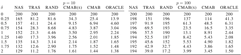
p= 10and∆ = 0.1forp= 100following the algorithm of Xian, Wang, and Liu (2017). Their performances for the two change patterns are shown in Tables 1-2.
It is clear that for both change patterns in both settings, except for ORACLE that is infeasible in practice, CMAB
has the smallest ADD, followed by CMAB(s). Compared with these two schemes, RAND has weaker detection power, which validates the efficacy of the proposed adaptive sam-pling algorithm. However, when pis small (e.g.,p = 10), RAND still outperforms TRAS and NAS, indicating the su-periority of the proposed online change detection scheme for POMSCD. Furthermore, for the same shift magnitude, the proposed detection schemes (CMAB, CMAB(s), RAND and ORACLE) generally have better detection performance on pattern (ii) than pattern (i). This is reasonable since the detection power is largely determined by the Mahalanobis distance of the shifted mean vector from the normal one, i.e., ∆ = µ0cΣ−1µc. GivenΣ and the change patterns in our study, we have∆(ii) > ∆(i). However, as TRAS does
not consider the correlations of variables in the detection scheme, it is not expected to have a better detection result for pattern (ii) than pattern (i). For NAS, it has the weak-est detection power for pattern (i), since its tweak-est statistic is based on the ranks of different variables. When different variables shift in the same direction, their ranks will not change very much, and consequently NAS would have un-satisfactory performance.
To further examine the influence ofm on the detection performance, Table 3 shows the ADDs of different methods on change pattern (i) withδ= 0.5using differentm, in the settingp= 10. Clearly, asmincreases, all the methods have smaller ADDs, and their relative performances are similar to those in Tables 1-2, where CMAB has the best performance.
Case Study on Real-world Data
We use a real data set from a semiconductor manufacturing process to demonstrate the application of our methodology. The data set is publicly available in UCI Machine Learning Repository (http://archive.ics.uci.edu/ml/datasets/SECOM). It contains in total 1,567 wafer samples from a semicon-ductor manufacturing process. Among them, 1,463 samples are classified as conforming ones (normal samples), while the remaining 104 samples are classified as nonconforming ones (abnormal samples). After preprocessing, each sample consists of measurements of 31 variables in each wafer pro-duction. Figure 1 shows the correlations of the 31 variables calculated based on all normal samples. We can see that different variables have strong cross-correlations with each other. This indicates considering variable correlations in the anomaly detection scheme is essential.
We construct the online change detection context as fol-lows: for every simulation replication, at each sensing epoch
t < τ, we draw a sampleX(t)from the 1,463 normal sam-ples randomly and sequentially with replacement. At each sensing epochτ ≤t, we draw a sampleX(t)from the 103 abnormal samples randomly and sequentially with replace-ment. We setτ = 50. Furthermore, though the data set has a total of31variables for each sample, in our experiment, we assume onlymout of31variables can be observed for each
signif-Table 1: Average Detection Delays (ADDs) of different methods for change pattern (i).
p= 10 p= 100
δ NAS TRAS RAND CMAB(S) CMAB ORACLE NAS TRAS RAND CMAB(S) CMAB ORACLE
0 200 200 200 200 200 200 200 200 200 200 200 200 0.25 165 81.2 81.6 34.3 25.4 13.9 198 151 196 137 114 41.3 0.5 157 41.1 24.4 9.15 6.94 4.60 197 91.9 195 61.3 48.5 6.31 0.75 154 28.3 8.68 4.83 3.87 3.04 196 69.5 193 23.5 16.5 3.35 1 152 21.3 4.46 3.50 2.95 2.24 196 57.5 190 13.1 8.91 2.44 1.25 140 17.3 3.96 2.56 2.01 1.85 194 52.5 187 8.42 5.43 2.08 1.5 135 14.3 3.14 2.14 1.87 1.65 195 45.6 152 5.53 4.90 1.82 1.75 132 12.6 2.90 1.75 1.52 1.48 192 42.9 32.7 4.43 3.86 1.65 2 129 11.2 1.76 1.61 1.44 1.38 194 39.0 17.2 3.99 3.45 1.50
Table 2: Average Detection Delays (ADDs) of different methods for change pattern (ii).
p= 10 p= 100
δ NAS TRAS RAND CMAB(S) CMAB ORACLE NAS TRAS RAND CMAB(S) CMAB ORACLE
0.25 109 119 55.4 24.1 19.4 10.6 168 178 198 136 112 30.3 0.5 50.5 81.1 16.8 6.97 5.03 3.64 87.3 90.7 196 63.5 49.3 5.03 0.75 28.5 40.6 7.50 4.08 3.12 2.50 57.2 68.9 195 18.4 11.2 3.23 1 19.5 28.1 4.60 3.13 2.21 2.01 36.2 57.0 193 9.12 5.32 2.42 1.25 15.1 21.2 3.12 2.34 2.01 1.84 29.5 49.7 190 5.78 4.14 1.93 1.5 13.3 17.3 2.62 2.07 1.98 1.61 20.1 45.1 101 4.27 3.64 1.69 1.75 11.7 14.1 2.22 1.84 1.72 1.58 19.6 42.3 24.8 3.98 2.95 1.65 2 11.3 12.6 1.92 1.71 1.64 1.57 17.5 38.8 14.9 3.11 2.49 1.48
variable index 5 10 15 20 25 30
variable index
5
10
15
20
25
30 0.1
0.2 0.3 0.4 0.5 0.6 0.7 0.8 0.9 1
Figure 1: Correlations of the 31 variables of normal samples in the real-world data application.
icantly outperform the baselines. This further confirms the superiority of the proposed methodology.
Conclusions
This paper presented a novel unsupervised online learn-ing scheme for Partially Observable Multi-senor Sequential Change-point Detection (POMSCD) in the context of lim-ited sensing resources available for monitoring changes of a system with multivariate streaming data. We tackled two open challenges of POMSCD: (i) how to construct an effec-tive online change-point detection scheme from multi-sensor data streams with partial observations; and (ii) how to adap-tively allocate sensing resources to collect the most informa-tive observation in order to maximize the detection power.
Table 3: ADDs of different methods for pattern (i) with dif-ferentmforδ= 0.5inp= 10.
m NAS TRAS RAND CMAB(s) CMAB 3 185 78.2 31.6. 20.3 15.2 5 157 41.1 24.4 9.15 6.94 7 78.2 36.5 14.1 7.25 6.12 9 42.1 28.7 10.0 6.24 5.21 10 21.4 19.1 7.24 5.15 4.85
Table 4: ADDs of different methods on the real data set.
m NAS TRAS RAND CMAB(s) CMAB 3 158 91.7 62.4 59.1 37.4 5 132 71.5 48.3 44.3 28.0 10 121 55.7 41.3 39.1 24.2 20 114 48.2 35.9 29.1 19.9 30 106 40.1 30.4 24.1 16.4
Acknowledgements
This research is supported by the National Research Foun-dation Singapore under its AI Singapore Programme [AISG-RP-2018-001]. This work was done when Chen Zhang worked at Dr. Hoi’s research group at SMU.
References
Bubeck, S.; Wang, T.; and Viswanathan, N. 2013. Multi-ple identifications in multi-armed bandits. InInternational Conference on Machine Learning, 258–265.
Chan, H. P. 2017. Optimal sequential detection in multi-stream data. The Annals of Statistics45(6):2736–2763. Chen, W.; Wang, Y.; Yuan, Y.; and Wang, Q. 2016. Combi-natorial multi-armed bandit and its extension to probabilis-tically triggered arms. The Journal of Machine Learning Research17(1):1746–1778.
Durand, A., and Gagn´e, C. 2014. Thompson sampling for combinatorial bandits and its application to online feature selection. InWorkshops at the Twenty-Eighth AAAI Confer-ence on Artificial IntelligConfer-ence.
Even-Dar, E.; Mannor, S.; and Mansour, Y. 2006. Ac-tion eliminaAc-tion and stopping condiAc-tions for the multi-armed bandit and reinforcement learning problems.Journal of ma-chine learning research7(Jun):1079–1105.
Gai, Y.; Krishnamachari, B.; and Jain, R. 2010. Learning multiuser channel allocations in cognitive radio networks: A combinatorial multi-armed bandit formulation. InNew Frontiers in Dynamic Spectrum, 2010 IEEE Symposium on, 1–9. IEEE.
Hoi, S. C.; Sahoo, D.; Lu, J.; and Zhao, P. 2018. Online learning: A comprehensive survey. CoRRabs/1802.02871. Kapoor, A.; Grauman, K.; Urtasun, R.; and Darrell, T. 2007. Active learning with gaussian processes for object catego-rization. InComputer Vision, 2007. ICCV 2007. IEEE 11th International Conference on, 1–8. IEEE.
Komiyama, J.; Honda, J.; and Nakagawa, H. 2015. Optimal regret analysis of thompson sampling in stochastic multi-armed bandit problem with multiple plays. InInternational Conference on Machine Learning, 1152–1161.
Liu, K.; Mei, Y.; and Shi, J. 2015. An adaptive sam-pling strategy for online high-dimensional process monitor-ing.Technometrics57(3):305–319.
Montgomery, D. C. 2009.Introduction to statistical quality control. John Wiley & Sons (New York).
Nelson, B. L.; Swann, J.; Goldsman, D.; and Song, W. 2001. Simple procedures for selecting the best simulated system when the number of alternatives is large. Operations Re-search49(6):950–963.
Tartakovsky, A. G.; Rozovskii, B. L.; Blazek, R. B.; and Kim, H. 2006. A novel approach to detection of intrusions in computer networks via adaptive sequential and batch-sequential change-point detection methods. IEEE Transac-tions on Signal Processing54(9):3372–3382.
Tartakovsky, A.; Nikiforov, I.; and Basseville, M. 2014. Se-quential analysis: Hypothesis testing and changepoint de-tection. Chapman and Hall/CRC.
Wang, J.; Zhao, P.; Hoi, S. C.; and Jin, R. 2014. Online feature selection and its applications.IEEE Transactions on Knowledge and Data Engineering26(3):698–710.
Xia, Y.; Qin, T.; Ma, W.; Yu, N.; and Liu, T.-Y. 2016. Bud-geted multi-armed bandits with multiple plays. InIJCAI, 2210–2216.
Xian, X.; Wang, A.; and Liu, K. 2017. A nonparametric adaptive sampling strategy for online monitoring of big data streams. Technometrics1–12.
Xie, Y., and Siegmund, D. 2013. Sequential multi-sensor change-point detection. The Annals of Statistics41(2):670– 692.
Zhou, D. P., and Tomlin, C. J. 2018. Budget-constrained multi-armed bandits with multiple plays. InAAAI.