The Thirty-First AAAI Conference on Innovative Applications of Artificial Intelligence (IAAI-19)
Discovering Temporal Patterns from Insurance Interaction Data
Maleeha Qazi,
2Srinivas Tunuguntla,
1Peng Lee,
2Teja Kanchinadam,
2Glenn Fung,
2Neeraj Arora
11University of Wisconsin - Madison 2American Family Insurance
{stunuguntla,neeraj.arora}@wisc.edu,{mqazi,plee,tkanchin,gfung}@amfam.com
Abstract
In the insurance industry, timely and effective interaction with customers are at the core of everyday operations and pro-cesses that are key for a satisfactory customer experience. These interactions often result in sequences of data derived from events that occur over time. Such recurrent patterns can provide valuable information that can be used in a variety of ways to improve customer related work-flows. In this paper we demonstrate the application of a recently proposed algo-rithm to uncover such time patterns that takes into account the time between events to form such patterns. We use temporal customer data generated from two different use-cases (satis-faction and fraud) to show that this algorithm successfully detects patterns that occur in the insurance context.
1
Motivation/Introduction
Recurrent patterns in event sequences occur in diverse con-texts that include notes in a musical composition, moves such as give-and-go in sports and turn-taking behavior ex-hibited by humans. In a retail context, buyers may engage in predictable on-line browsing behavior patterns before mak-ing a purchase. Similarly, in many processes and work-flows in the insurance industry, policyholders of an insurance provider may experience distinct patterns of interactions as they navigate the claims process. Examples of events during this process include claim reporting, bill paying, adding a coverage, and general inquires. Patterns extracted from the temporal data in the claims process reveal insights that could be used to optimize customer interactions and enhance the overall customer experience with the insurance company. The purpose of this paper is two fold:
1. To introduce the recently proposed scalable T-pattern al-gorithm (Arora, Fung, and Tunuguntla 2017) that has been proposed in a business setting to the AI and data mining community and to relate it to other similar meth-ods for temporal discovery.
2. To showcase how this proposed algorithm can be used to extract patterns from temporal sequence data that arise in the insurance domain.
The recently proposed algorithm (Arora, Fung, and Tunuguntla 2017) builds upon prior work (Magnusson 2000)
Copyright c2019, Association for the Advancement of Artificial Intelligence (www.aaai.org). All rights reserved.
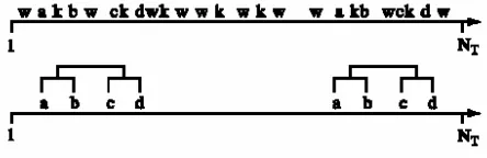
Figure 1: Illustration from (Magnusson 2000)
which defined the term T-pattern as a sequence of events that occur with a relatively consistent time interval between each event and where the sequence appears in the data more often than one would statistically expect by chance alone. The time dimension adds significant complexity to the task of detecting patterns in any data, and identifica-tion of such patterns becomes quite difficult for even mod-est sized data. Most algorithms known in the data mining community either assume that the time intervals between events is constant (Mannila, Toivonen, and Inkeri Verkamo 1997), or ignore the time intervals between events and fo-cus only in the sequential order of the events (Zaki 2000; 2001).
A simple illustration from (Magnusson 2000) helps mo-tivate the thinking behind a T-pattern. In this illustration, there are six events (a, b, c, d, w, k)that occur several dif-ferent times during the period[1, NT]as shown in the first
row in Figure 1. The second row reveals the time pattern among some of the variables. At the first level of the hier-archy, two T-patterns are found: [a, b] and[c, d]. The sec-ond level of the hierarchy reveals one more T-pattern:[a, b],
[c, d]. Even in this simple example, the underlying T-pattern is not self-evident from the observed data. As we will show, under this paradigm, the problem of detecting a T-pattern gets exponentially difficult as the number of events in the data increase.
scalable to typical business problems that have a large num-ber of events and individuals.
In (Arora, Fung, and Tunuguntla 2017) we conducted simulations to exhibit the properties of the proposed algo-rithm and it’s ability to recover patterns when the true T-patterns are known. In the empirical section of this paper, section 6, we test the algorithm using customer insurance data derived form two different use-cases. The final section of the paper summarizes the main aspects of the paper and offers conclusions.
2
Related Work
Over the years the T-pattern algorithm has been applied in a variety of contexts to study interactions and behavior in-volving animals and humans. (Casarrubea et al. 2015) does an excellent job of summarizing these applications. The re-search involving T-patterns and humans span topics such as cognitive and social disorders, gender relations, team effec-tiveness, and sports. In their paper on T-patterns involving performance of soccer teams, (Borrie, Jonsson, and Mag-nusson 2002) observe that traditional analyses focus on fre-quency of event occurrence (e.g. number of passes, assists, unforced errors, etc.) as the index of performance. What’s missing from such analyses, they note, is the temporal struc-ture and interrelationships between events. Using the T-pattern approach, the authors point to the importance of tem-poral aspects of sports performance that reveal novel pat-terns that impact team performance. We believe that such temporal patterns are widely prevalent in business applica-tions and are important to study.
In (Batal et al. 2016), the authors present Recent Tempo-ral Pattern (RTP) mining as a “novel approach for efficiently finding predictive patterns for event detection problems” in complex multivariate temporal data like electronic health records (EHRs). Although their methodology has some sim-ilarities to our approach, for example using supervised prun-ing to help scalability, easy interpretability of detected pat-terns, and bottom-up detection of patpat-terns, their technique is built on the assumption that more recent patterns are more predictive than past patterns. This assumption holds for the medical domain but doesn’t necessarily apply to domains such as insurance. Also, their algorithm requires abstracting the concept of time in two different ways: trend abstractions and value abstractions. In addition, the concept of “recent” is declared using a user-defined parameter. Our algorithm, in contrast, is not limiting in this aspect. Time doesn’t require a user-defined restriction or abstraction in our approach and the purpose of our algorithm is to find the most salient time boundaries to define the detected patterns.
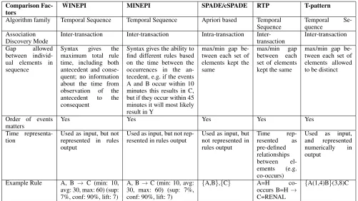
Various algorithms known in the data mining commu-nity have been compared to one another in previous sur-veys (Roddick and Spiliopoulou 2002; Mooney and Roddick 2013). In Table 1 we chose three well known algorithms, WINEPI/MINEPI (Mannila, Toivonen, and Inkeri Verkamo 1997), SPADE/cSPADE (Zaki 2000; 2001) & RTP (Batal et al. 2016), to compare against our algorithm along some key dimensions of interest. As can be seen, WINEPI/MINEPI & SPADE/cSPADE do not represent time explicitly in their output rules. Although RTP does represent time in its output
rules, it is re-represented as pre-defined relationships (e.g. co-occurs, contains, etc.) This is a common trend for time series data. It can limit the knowledge the rules can represent to what a human has given an algorithm access to represent. If knowledge isn’t represented at the correct granularity for learning, then the algorithm cannot produce the desired re-sults. This is one of the reasons we allow time to remain as-is within our algorithm.
As far as we know, our proposed algorithm is the only algorithm (other than Magnusson’s) that considers both or-der and variable time between events, without having to re-represent time in any way, & while being able to scale to address the demand of many present-day business problems.
3
Original T-pattern Algorithm
We begin this section by formalizing the definitions used by our proposed algorithm (Arora, Fung, and Tunuguntla 2017) and the algorithm proposed by (Magnusson 2000). Let event
ioccur for personj during timet. We define the following variable to capture the occurrence of event typeE.
Eijt =
1 if eventifor personjoccurs during timet 0 otherwise
(1) As an example, for four individuals (P1toP4) and nine
event types (E1toE9). Fori= 1, ...,9events, the possible
set of T-patterns isQand includes all possible event combi-nations.
Q={(E1, E2),(E1, E3), ..,(E8, E9), ..,(E1, E2, .., E9),
..,(E2, E1), ..,(E9, .., E3, E2, E1)}
(2)
The goal is to detect T-patterns such as(E1, E2)that
fol-low the definition that a T-pattern is (i) a sequence of events that occur with a relatively consistent time interval between each event and (ii) where the sequence appears in the data more often than one would statistically expect by chance alone. We use the subscriptkto refer to a T-pattern where
k∈ {1, ..., K}is a small subset of all possible event combi-nations inQ.
The T-patterns are not expected to follow a deterministic time pattern. That is, the inter-event time maybe stochastic. One of our goals is to find acritical intervalthat corresponds to each T-pattern. Formally, for a two-event T-patternkwe will uncover the interval(ck1, ck2)such that the second
ele-ment of the T-pattern falls somewhere betweent=ck1and
t = ck2 after the first element. For example,E1(4,10)E2
implies thatE2is likely to occur4to10time units afterE1.
The same notations naturally extends to longer T-patterns that exceed two events. For example,E3(3,11)E5(2,5)E7
implies thatE5is likely to occur3to11time units afterE3
andE7is likely to occur2to5time units afterE5.
3.1
Magnusson’s Algorithm
For any pair of eventsEiandEi0, next we outline how the
Table 1: Comparison of Various Algorithms
Comparison Fac-tors
WINEPI MINEPI SPADE/cSPADE RTP T-pattern
Algorithm family Temporal Sequence Temporal Sequence Apriori based Temporal Sequence
Temporal Se-quence
Association Discovery Mode
Inter-transaction Inter-transaction Intra-transaction Inter-transaction
Inter-transaction
Gap allowed
between individ-ual elements in sequence
Syntax gives the maximum total rule time, including both antecedent and conse-quent; no information about the time from observation of the antecedent to the consequent
Syntax gives the ability to find different rules based on the time between the occurrences in the an-tecedent, e.g. if the events A and B occur within 10 minutes this results in C, but if they occur within 45 minutes it will most likely result in Y
max/min gap be-tween each set of elements kept the same
max/min gap between each set of elements kept the same
max/min gap be-tween each set of elements allowed to be distinct
Order of events matters
Yes Yes Yes Yes Yes
Time representa-tion
Used as input, but not represented in rules output
Used as input, but not rep-resented in rules output
Used as input, but not represented in rules output
Time
rep-resented as pre-defined relationships between el-ements (e.g. co-occurs)
Used as input, and represented numerically in output
Example Rule A, B → C (min: 10, avg: 30, max: 60) (sup: 7%, conf: 90%, lift: 7)
A, B→C (min: 10, avg: 30, max: 60) (sup: 7%, conf: 90%, lift: 7)
{A,B},{C} A=H co-occurs B=H→ C=RENAL
{A(1,4)B}(3,8)C
T-pattern is based on the null hypothesis that the two events
EiandEi0 are distributed independently with the observed
frequency during the observation period[1, T]. The follow-ing probabilities are necessary to test for the presence of T-pattern (Ei, Ei0). The marginal probabilities for Ei0 are
given by:
P r(Ei0 = 1) =
NEi0
NT
;P r(Ei0 = 0) = 1−
NEi0
NT
(3)
For the eventEi, let us focus our attention on an arbitrary
interval[c1, c2]that followsEi. The probability that one or
more eventsEi0 lie in the interval[c1, c2]that followsEi, is
calculated as follows,
P r(Ei0 ≥1|c1, c2) = 1−(1−
NEi0
NT
)c2−c1+1 (4)
LetnEi,Ei0 be the number of instances whenEi0 occurs
within the interval [c1, c2]after Ei. Using equation 4, one
can calculate the probability distribution ofnEi,Ei0.
P r(nEi,Ei0 =n|c1, c2) =Binomial(NEi, n, P r(Ei0 = 1|c1, c2))
(5)
For theNEi occasions that eventEioccurs, the expected
number of times the event Ei0 occurs within the interval
[c1, c2]afterEican be written as
E(nEi,Ei0) =NEi×(1−(1− NEi0
NT
)c2−c1+1) (6)
Given that we observe the number of times Ei0 occurs
within the interval[c1, c2], the probability that the(Ei, Ei0)
isnota T-pattern is given below.
p= 1−
NEi,Ei0−1
X
n=0
Binomial(NEi, n, P r(Ei0= 1|c1, c2))
(7) This is also the probability of the null hypothesis that the two events Ei andEi0 are distributed independently to be
true. Therefore, small values ofpin Magnusson’s algorithm indicate evidence in support of a T-pattern.
The algorithm begins by recording the time until the near-est occurrence of Ei0 afterEi and defines the distribution
of these distance intervals. In doing so, it ignores any event that occurs betweenEiandEi0. Then, the algorithm checks
all the possible time intervals (ck, ck0) where Ei0 occurs
after Ei for statistical significance. If an interval is found
to be significant based upon the test criterion explained in Equation 7, the candidate patternEi(cl, cl∗)Ei0 is called a
T-pattern and saved as a candidate to be part of a more com-plex t-pattern in future iterations.
3.2
Limitations of Magnusson’s Algorithm
The original algorithm suffers from a series of limitations when applied to typical business contexts, and we outline them here:for data that are larger in scope - including many individ-uals and events. As the number of events and individindivid-uals increase, the algorithm breaks down because the number of combinations increase exponentially.
2. Heterogeneous individuals: The original algorithm fails to recognize that events occur at different frequencies for different individuals. As a result, the algorithm uncovers T-patterns that exhibit long critical intervals that do not occur very frequently.
3. Distributional assumptions: The test for a patternEi,
Ei0 is based on the null hypothesis that the two events
are independent Bernoulli processes over the observation period with constant probabilities of occurrence within a time unit. The original algorithm (see Equation 3) uses this to calculate the probability of an event Ei0
occur-ring in the interval [d1, d2]after an eventEi. We note
that, since the nearest occurrences of Ei0 after Ei are
used to calculate the distance intervals, under the null hypothesis, these distance intervals should be geometri-cally distributed. We incorporate this correction from the Bernoulli to a geometric distribution in the algorithm.
4
A Revised T-pattern Algorithm
Our revised T-pattern algorithm is documented in (Arora, Fung, and Tunuguntla 2017) and offers several improve-ments to address the limitations pointed out above. These improvements are summarized below.
4.1
Scalability
Our proposed algorithm addresses this problem by: (a) op-tionally incorporating the use of labels in a supervised man-ner to discard patterns that have poor or no discriminative value for classification problems, (b) proposing an adequate data structure that makes calculations more tractable, and (c) parallelizing the algorithm. In this section we will focus on (a) while (b) and (c) will be addressed in section 5.
A challenging aspect of typical business applications is that the number of individuals and events maybe large. For example, the data we use in our experimental section involves thousands of samples (individuals, observations), hundreds of event types, and millions of total event occur-rences. This imposes substantial computation burden on the algorithm. The challenge is presented by the large set size for Q (the total number of T-pattern candidates to evalu-ate) and critical interval determination for each possible T-pattern. Our proposed solution to tackle this combinatorial hurdle is to use “smart” pruning. For our revised T-pattern algorithm, both unsupervised and supervised pruning proves valuable in scaling and hence avoiding, or reducing, the pos-sibility of a combinatorial explosion that may lead to in-tractability.
When applyingunsupervised pruningthe idea is pretty simple: T-patterns that may have very low event counts or are associated with events with significant low counts may offer little or no information. In contrast, their inclusion may result in substantial computational cost. For industrial appli-cations, an important application for T-patterns is in the area of classification problems.
When applying supervised pruning, we are interested in measuring the information gain from the occurrence of a candidate pattern(Ei, Ei0)to a given label by using the
Kullback-Leibler (KL) divergence criterion (Kullback and Leibler 1951). This allows us to uncover T-patterns that are likely candidates to be the drivers of the difference between two classes. Such a supervised pruning approach is gen-eral and could be applied to any classification target variable or label (e.g. satisfied/unsatisfied customers, loyal/switchers, etc.).
4.2
Heterogeneous Individuals
To account for the fact that the number of events per indi-vidual vary, the probability of an eventEi0 occurring in the
interval[c1, c2]afterEiis calculated at the individual level.
Unlike the binomial distribution that involves a sequence of Bernoulli trials with the same success probability for each individual, the Poisson Binomial distribution involves a se-quence of Bernoulli trials with a different success probabil-ity for each individual. So we chose to replace the use of the Bernoulli distribution with the Poisson Binomial distri-bution.
Hence, the evidence against the T-pattern is given by
p= 1−
NEi,Ei0−1
X
n=0
P oissonBinomial(NEi, n, P r) (8)
Small values of p indicate evidence in support of a T-pattern.
4.3
Distributional Assumptions
Starting at an arbitrary point in time, the distance of the first occurrence of event Ei after that point, follows a
geomet-ric distribution with success probabilityPEi. Similarly, the
distance to the first occurrence of event Ei0 after Ei,
fol-lows a geometric distribution with parameterPEi0. An event
Ei0 is paired with an eventEi, at a distancedonly if it is
the first occurrence ofEi0 afterEi. It can be shown (Arora,
Fung, and Tunuguntla 2017) that the probability of an event
Ei0occurring in the interval[c1, c2]after an eventEican be
calculated as
P r(c1≤D≤c2) =P r(D≤c2)−P r(D≤c1−1)
= (1−pdist)c1−1−(1−pdist)c2
(9) We therefore replace Equation 4 by Equation 9 in the origi-nal algorithm.
4.4
CI Search Stopping Criteria
4.5
Summary of Proposed Algorithm
We start by treating each event type as a 1-event T-Pattern. For each event type, the start time and end time for each of its instances are recorded for all the individuals in the dataset. In general, a candidate pattern is of the form(Pi, Pj)where
Pi,Pj are two T-Patterns found in the data. The algorithm
can be summarized in the following steps:
Algorithm 1Revised Scalable T-pattern Algorithm Input: Vector of targets or labelsL-{l1, l2, . . . , lm}
Matrix of eventsM
Output: Final list of T-patterns
1: Create a list of candidate patternsC.
2: foreach candidate pattern(Pi, Pj)∈C do
3: Create a list of event pair instances for all the in-dividuals. The event pair instances are of the form
(Pi(d)Pj), wheredis the distance between the event
instancesPi,Pj.
4: Evaluate if the candidate pattern is a T-Pattern.
5: ifCandidate is a t-patternthen
6: calculate the critical interval (d1, d2)and add the
pattern(Pi,Pj)to the list of found T-PatternsT.
7: end if
8: add the top-k features to the BN in a Naive Bayes fashion.
9: end for
10: Go to step (1) if any new T-Patterns are found in step (2)
11: return T
5
A Parallel and Scalable Implementation
5.1
Data Structures
In algorithm 1, step (3), for a given candidate pattern
(Pi, Pj), we create a list of all event pair instances of the
form (Pi(d)Pj), where d is the distance between the end
time of an instance ofPiand the start time of the instance of
Pjthat immediately follows. To improve the computational
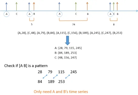
efficiency of this step, we use the following data structure to store data corresponding to any pattern (see Figure 2). The instances of the pattern are stored in the increasing order of their times of occurrence. The order is the same irrespec-tive of using the start times or the end times of the instances to sort, because the instances are non-overlapping. For each instance, the start and end times are recorded.
For a given candidate pattern (Pi, Pj), to calculate the
event pair instances as in algorithm 1, step (3), it is sufficient to perform a simultaneous linear search on the instances of both the patterns, because the instances are sorted. The event pair instances now form the instances of the candidate pattern (Pi, Pj). The start time of an instance of the form
(Pi(d)Pj)is the start time of the instance ofPi. Similarly,
the end time of the instance is the end time of the instance ofPj. If the candidate pattern is found to be a T-Pattern with
critical interval(d1, d2), the event pair instances that satisfy
d1≤d≤d2are collected, sorted and stored as data for the
new T-Pattern.
Figure 2: Data Restructuring: Start with events stored in the increasing order of their times of occurrence, then sample pairs to see if pattern exists.
5.2
Parallel Implementation
With large datasets that include many event types, the algo-rithm requires significant computation because of the need to evaluate many candidate patterns. With the ease of access to cloud computing and the availability of multiple cores on each computer, parallelization can be used to speed up the algorithm significantly.
In algorithm 1, step (2), we evaluate whether each of the candidate patterns is a T-Pattern. The evaluation of a candi-date pattern is independent of the evaluation of other can-didate patterns. Hence, this step can be easily parallelized. Each candidate pattern can be processed on a different core of a computer. In the implementation, a master thread and a number of worker threads are used to evaluate candidate pat-terns efficiently. The master thread creates a queue of candi-date patterns. This is a FIFO queue and is serviced by the worker threads. The worker threads watch the queue and pick up a candidate pattern to evaluate whenever they be-come available. If a candidate pattern is found to be a T-Pattern, it is returned to the master thread. All the T-Patterns that are found in Algorithm 1, step (2) are collected by the master thread and the process is repeated. We use a cluster of 16 computers that use Message Passing Interface (MPI) pro-tocol to communicate. MPI is a communication propro-tocol that supports both point-to-point and collective communication in parallel programming. Each computer has 16 cores and has its own private memory of 60 GB. We choose the MPI protocol over the others because it allows the computers in the cluster to read data in parallel and store it in their private memory. The use of the cluster reduced the run time of the algorithm from approximately 16 days on a single computer to less than 2 hours.
6
T-patterns from Insurance Work-flows
6.1
Customer Satisfaction
We selected claims data from a well-known insurance com-pany to test the T-pattern algorithm. In order for an insurance policy holder to get reimbursed for a loss or an incident, a claim has to be filed. The claim process usually consists of a series of events and interactions that involve the insurance company, the insured, and various third parties. The process ends shortly after a payment is adjudicated.
According to Accenture in their news release of Oct. 13, 2014: “83 percent of dissatisfied customers [after a claim] are planning to switch or have already switched to another insurer”. Given that the insurance company mentioned had 142K property and 644K auto claims submitted in 2014, even with low levels of dissatisfaction, capturing these early on can result in fewer households leaving the company af-ter a claim. This in turn can translate to roughly 4 million dollars in business a year.
We use the concept of a journey-map as a data-driven structured time-line where all the events pertinent to the claim process are identified and positioned temporally with respect to each other. To generate the dataset used for this problem we created claim maps. These journey-maps integrate events from different data sources that are available during the claim process. Most of these events are internal to the company and some involve the customer or a third party (e.g. a car repair shop). We have two primary pur-poses in these analyses. First, we want to show that the pro-posed algorithm can detect T-patterns that routinely occur in the context of insurance claims. This would serve as a face validity check for the algorithm. Second, we want to uncover T-patterns that separate dissatisfied customers from satis-fied ones. Such T-patterns may help identify touch-points that could help minimize customer dissatisfaction with the claims process.
We used data from auto and property claims in our anal-ysis. Upon completion of the claim process each customer filled out a satisfaction survey. In total, there are 166,504 claims in our data, of which 7,874 (4.73%) customers indi-cated that they were dissatisfied with the claims process. Of these, 109,031 claims belonged to the auto category (3.2% dissatisfaction), and 57,473 claims belonged to the property category (7.6% dissatisfaction).
There are a total of 236 event types in our data (232 for auto, 202 for property), 12,758,448 event instances (8,965,952 for auto, 3,792,496 for property) and, on aver-age, 86 event instances/claim.
Both the auto and property datasets were split into 60/40 train/test sets. Then the algorithm was run on each training set separately. We used a p-value threshold of 0.01 and set the pruning cutoffs at 2.84% of the total event instances in each train set. For our experiments we allowed the cutoff for infrequent events and the cutoff for infrequent pairs be the same value. A smaller cut-off results in a substantially larger number of T-patterns, that increases the run-time for the algorithm exponentially. In addition, the KL divergence cutoff was varied between 0.01 and 0.000625. The primary benefit of the KL cutoff is that it helps identify the T-patterns that are more likely to discriminate between satisfied and dissatisfied customers.
Table 2: Auto & Property AUCs for Train/Test sets; super-vised runs with varying KL cutoff parameter, best results shown at KL cutoff of 0.00125. Best performance inbold.
TP (= T-pattern). BOW (= Bag-Of-Words) features are basic counts of each event. We excluded adding any aggregate fea-tures (e.g. total number of events in claim, number of unique events in claim, duration of claim, etc.) for simplicity of com-parison.
Feature Set Algo Auto Train Auto Test Prop Train Prop Test
TP GB 0.744 0.714 0.720 0.678 BOW GB 0.771 0.747 0.739 0.703 BOW+TP GB 0.783 0.753 0.757 0.721
cSPADE GB 0.757 0.523 -
-Next, we used each discovered T-pattern as a binary fea-ture to classify satisfied and dissatisfied customers. Using these features, we trained 4 different scikit-learn (Pedregosa et al. 2011) (version 0.18) models: Logistic Regression with L1 penalty (LogR L1), Logistic Regression with L2 penalty (LogR L2), Random Forest (RF; with 100 estimators, and out-of-bag sampling set to True), and Gradient Boosting Classifier (GB). Each algorithm used it’s default parame-ter settings unless otherwise specified here. The best results were consistently obtained with GB so for the rest of the pa-per we will only report GB results. The training set is used to generate the T-Patterns. The binary features correspond-ing to these T-Patterns are used to build a model over the training set. The model is then used to predict satisfaction of claimants in the hold-out/test set.
We use a simple summary measure of binary preci-sion/recall: Receiver Operating Characteristic (ROC) curves (Fawcett 2006), and report Area Under the ROC Curve (AUC) as our prediction measure. The prediction results for GB can be seen in Table 2. This shows that the pres-ence/absence of these T-Patterns are a good indicator of sat-isfaction. Example T-Patterns can be seen in Table 3.
We compare our algorithm’s result against a classic fre-quent sequence mining algorithm called cSPADE (Zaki 2000). We used the R packageaRulesSequencesto run the cSPADE code against our datasets (R Core Team 2018; Hahsler et al. 2018; Hahsler, Gruen, and Hornik 2005; Hahsler et al. 2011). This algorithm was chosen because it represents sequence mining that takes into account the or-der of events, but not the variable time between events - an aspect of our algorithm which we believe is distinguishing. This would allow for the closest possible match for the sake of comparison between algorithms and it would help illus-trate why variable time between events is desirable to in-clude. (Zaki 2000) states that the cSPADE algorithm can be run with a constraint to handle classes, and we chose to run the algorithm with this constraint so the results would be comparable to our supervised runs. The results can be seen in Table 2. Note that cSPADE cannot handle datasets with events that only occur in the testset but are never seen in the training set, hence we could not generate results for the property dataset.
Table 3: Example T-patterns from Auto & Property Data T-patterns
Auto (ClaimReported 1,7 (VehicleEdited 1,22 ClaimClosed))
Auto (ClaimReported 1,28 ((Suspense 1,8 ClaimClosed) 1,56 grpPymtSubmit)) Prop ((ClaimSetup 1,14 ClaimClosed) 5,51
As-sociatedToParty)
Prop ((ClaimSetup 1,57 (FYISent 1,7 Sus-pended Item)) 5,53 ClaimReopened)
1. The first example shows that changes to the vehicle de-scription/condition were made 1 to 7 days after a claim is reported, and within 1 to 22 days after that the claim was closed. This is correlated with a bad assessment or a complicated claim.
2. The second example shows a claim that was reported and paid for after 1-2 months via a batch payment method. 3. The third example shows a claim setup and closure within
1 to 14 days, but associated to an internal handler 5 to 51 days after closure. This correlates with a complicated claim not going smoothly and/or swiftly.
4. The forth example shows a claim which was suspended for a long time during it’s resolution process, and then reopened 5 to 53 days after it was closed. This is a pattern from a slow moving claim.
physical CPU cores (note that this R session was one of mul-tiple processes occupying the machine at runtime). Lower support values would error out for various reasons.
As was the case for T-pattern detection, we used the train-ing set to generate the sequences. The binary features cor-responding to the sequences was used to build a model over the training set, and the model was then used to predict sat-isfaction in the test set. As can be seen by the testset AUCs, cSPADE doesn’t do as well with the classification task as our T-pattern algorithm. Clearly the order of events alone (in cSPADE) isn’t as discriminative as when the time aspect is also taken into account (in T-patterns).
6.2
Fraud Detection
Insurance fraud is an act committed by a party, resulting in an unlawful gain from an insurance company. Parties who may commit fraud include insurance applicants, policyhold-ers, third-party claimants, professionals rendering services during the claims process such as doctors, lawyers and chi-ropractors, or other parties associated with a claim such as a witness in an accident. The majority of insurance com-pany respondents in a 2013 survey conducted by FICO es-timate that fraud can cost between 5% and 20% of claim volume. Hence, insurance companies are investing in auto-mated fraud detection solutions more so than ever before.
Automated insurance fraud detection solutions rely heav-ily on business rules derived by domain experts and features manually engineered by the data analyst. In some cases, ar-bitrary time cutoffs are selected as part of the feature engi-neering process. For instance, a claim on a recently bound policy is a red flag. However, “recent” is usually an arbitrary
point selected by the analyst with input from the business expert. Our algorithm helps in the automation of hand en-gineered features, resulting in more robust and data-driven feature engineering.
In addition to automated feature engineering, there is de-sire by the Special Investigations Unit (SIU) for a white box solution where T-patterns provide information beyond sim-ply flagging a claim. The sequences of events detected by the T-patterns provide the necessary information for SIU triage to make quicker hand-offs to the next line of defense, the SIU investigator. In addition, the sequences of events found can be used as information to ultimately support the SIU inves-tigator in the mitigation of a claim. This stretches the value of the data beyond a simple model input or business rule.
The analysis in this paper was focused on private passen-ger auto (PPA) claims that were referred to, and reviewed by SIU, at the well-known insurance company mentioned pre-viously. The primary motivation for this analysis was to help in reducing the false positives of claims already referred to SIU. SIU was receiving about 70% of their leads from a par-ticular source. 89% of claims referred by this source were false positives. By ranking or prioritizing already referred claims, this can allow SIU triage to ignore claims of lower quality, while focusing their energy on those with higher quality. In addition, as discussed, T-patterns provide automa-tion in feature engineering, and visibility into the types of sequences of events that are associated with fraudulent activ-ity. This additional information can help SIU triage be more efficient in their review.
SIU referrals constitute roughly 1.5% of the total PPA claims population. In addition to claims information, the data includes policy and billing transactions, and claim his-tory. Each claim had a binary label indicating fraudulent or no fraudulent activity associated with the claim.
There were a total of 35,230 claims in the dataset, with 317 event types represented, and an overall fraud signal of 12.46%. The data were split into 70/30 train/test sets. Sim-ilar to what we did for the last set of experiments with the claims data, we used a p-value threshold of 0.01. We kept the cutoff for infrequent events and the cutoff for infrequent pairs to be of the same value. In addition, the KL divergence cutoff was varied between 0.01 and 0.000625.
We then used each discovered T-pattern as a binary fea-ture to classify fraud claims. We applied the same 4 models previously described. The training set was used to generate the T-Patterns, and build a model. The model is then used to predict if a claim was fraudulent or not on the hold-out/test set. The prediction results for the best algorithm (GB) can be seen in Table 4; we again used AUC as our prediction mea-sure. Our experiments indicate that for a signal ratio like we have in this dataset, a KL cutoff of 0.00125 provided the best pattern set. Example T-Patterns can be seen in Table 5.
Table 4: Fraud AUCs for Test sets; supervised runs with varying KL cutoff parameter, best results shown at KL cut-offs mentioned. Best performance inbold.H.E.F. = Human Engineered Features
Feature Set Algorithm AUC
TP GB 0.568
H.E.F. GB 0.744
H.E.F.+TP GB 0.759
Table 5: Example T-patterns from Fraud T-patterns
(backdated policy change 1,86 (loss occurrence 1,3 loss setup))
(payment late 1,3 payment process)
1. The first example shows that the customer made a policy coverage change that they asked to be backdated (i.e. ap-plicable from some day in the past vs. from the time of the request). Within 1 to 86 days later they experienced a loss, and 1 to 3 days after that they submitting a claim for that loss.
2. The second example shows a customer made a late pay-ment which was processed within 1 to 3 days. It is known that customers that are late for their payments are more likely to submit fraudulent claims.
7
Summary and Conclusions
We have successfully applied a recently proposed scalable T-pattern algorithm (Arora, Fung, and Tunuguntla 2017) to two relevant problems in the insurance industry. The patterns discovered not only provide a way to automatically extract features that can be used in a later stage for classification purposes, but also provide rules that can be easily interpreted by humans. We have also introduced the proposed T-Pattern algorithm to the A.I. community as a tool to consider when the task is to discover and understand patterns that occur in temporal data. Furthermore, as mentioned before, this algo-rithm is the only available choice (as far as we know) that considers both order and time between events, while being able to scale to address the demand of many present-day business problems.
In recent years, there have been significant advances re-lated to the use of deep learning architectures for model-ing temporal data. Specifically, recurrent neural networks (RNN) and long short term memory networks (LSTMs) are designed to learn temporal dependencies. Such methods work very well for a large variety of prediction problems, and are now used widely. However, there are two limitations of such approaches: (i) they need large amounts of labeled data to work and they can be difficult to train due to the enormous amount of parameters to be learned (this is typi-cally the case with deep learning architectures in general), (ii) they use black-box models that produce excellent accu-racy but the results from such models are difficult to under-stand and interpret by humans. Our proposed T-pattern ap-proach provides interpretable results for temporal data.
References
Arora, N.; Fung, G.; and Tunuguntla, S. 2017. T-patterns in busi-ness. Unpublished Manuscript. Available at SSRN: https://ssrn. com/abstract=3066839 or http://dx.doi.org/10.2139/ssrn.3066839. Batal, I.; Cooper, G. F.; Fradkin, D.; Harrison, J.; Moerchen, F.; and Hauskrecht, M. 2016. An efficient pattern mining approach for event detection in multivariate temporal data. Knowledge and Information Systems46(1):115–150.
Borrie, A.; Jonsson, G. K.; and Magnusson, M. S. 2002. Temporal pattern analysis and its applicability in sport: an explanation and exemplar data.Journal of sports sciences20(10):845–852. Casarrubea, M.; Jonsson, G.; Faulisi, F.; Sorbera, F.; Di Giovanni, G.; Benigno, A.; Crescimanno, G.; and Magnusson, M. 2015. T-pattern analysis for the study of temporal structure of animal and human behavior: a comprehensive review.Journal of Neuroscience Methods239:34–46.
Fawcett, T. 2006. An introduction to roc analysis.Pattern Recogn. Lett.27(8):861–874.
Hahsler, M.; Chelluboina, S.; Hornik, K.; and Buchta, C. 2011. The arules r-package ecosystem: Analyzing interesting patterns from large transaction datasets. Journal of Machine Learning Research
12:1977–1981.
Hahsler, M.; Buchta, C.; Gruen, B.; and Hornik, K. 2018. arules: Mining Association Rules and Frequent Itemsets. R package ver-sion 1.6-1.
Hahsler, M.; Gruen, B.; and Hornik, K. 2005. arules – A computa-tional environment for mining association rules and frequent item sets.Journal of Statistical Software14(15):1–25.
Kullback, S., and Leibler, R. A. 1951. On information and suffi-ciency.The annals of mathematical statistics22(1):79–86. Magnusson, M. S. 2000. Discovering hidden time patterns in be-havior: T-patterns and their detection.Behavior Research Methods
32(1):93–110.
Mannila, H.; Toivonen, H.; and Inkeri Verkamo, A. 1997. Dis-covery of frequent episodes in event sequences. Data Mining and Knowledge Discovery1(3):259–289.
Mooney, C. H., and Roddick, J. F. 2013. Sequential pattern min-ing – approaches and algorithms.ACM Comput. Surv.45(2):19:1– 19:39.
Pedregosa, F.; Varoquaux, G.; Gramfort, A.; Michel, V.; Thirion, B.; Grisel, O.; Blondel, M.; Prettenhofer, P.; Weiss, R.; Dubourg, V.; Vanderplas, J.; Passos, A.; Cournapeau, D.; Brucher, M.; Perrot, M.; and Duchesnay, E. 2011. Scikit-learn: Machine Learning in Python .Journal of Machine Learning Research12:2825–2830. R Core Team. 2018. R: A Language and Environment for Statis-tical Computing. R Foundation for Statistical Computing, Vienna, Austria.
Roddick, J. F., and Spiliopoulou, M. 2002. A survey of tempo-ral knowledge discovery paradigms and methods. IEEE Trans. on Knowl. and Data Eng.14(4):750–767.
Zaki, M. J. 2000. Sequences mining in categorical domains: In-corporating constraints. In9th ACM International Conference on Information and Knowledge Management.