Hierarchical Context Enabled Recurrent Neural Network for Recommendation

(1)

The Thirty-Third AAAI Conference on Artificial Intelligence (AAAI-19)

Hierarchical Context Enabled Recurrent Neural Network for Recommendation

Kyungwoo Song,

1∗

_{Mingi Ji,}

1∗

_{Sungrae Park,}

2

_{Il-Chul Moon}

1

1_{Korea Advanced Institute of Science and Technology (KAIST), Korea} 2_{Clova AI Research, NAVER Corp., Korea}

{gtshs2,qwertgfdcvb_}@kaist.ac.kr, [email protected], [email protected]

Abstract

A long user history inevitably reflects the transitions of per-sonal interests over time. The analyses on the user history require the robust sequential model to anticipate the tran-sitions and the decays of user interests. The user history is often modeled by various RNN structures, but the RNN structures in the recommendation system still suffer from the long-term dependency and the interest drifts. To resolve these challenges, we suggest HCRNN with three hierarchical con-texts of the global, the local, and the temporary interests. This structure is designed to withhold the global long-term interest of users, to reflect the local sub-sequence interests, and to attend the temporary interests of each transition. Be-sides, we propose a hierarchical context-based gate structure to incorporate ourinterest drift assumption. As we suggest a new RNN structure, we support HCRNN with a comple-mentarybi-channel attentionstructure to utilize hierarchical context. We experimented the suggested structure on the se-quential recommendation tasks with CiteULike, MovieLens, and LastFM, and our model showed the best performances in the sequential recommendations.

Introduction

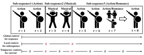
A user historyis a sequence of user orders or clicks, and the history represents the user’s interest. Given this user his-tory, many services such as movie recommendations, music streaming services, etc., are interested in recommending the next most likely click item. When we perform this recom-mendation, it has been assumed that the user’s interest can be hierarchically ranging from general interest to a temporary, specific need as shown in Figure 1. Here, these hierarchical interest dynamics are defined as 1) the global context for the entire sequence; 2) the local context for a sub-sequence, such as a click-stream of a site visit with a few or dozens of clicks; 3) and the temporary context for a transition of items. The assumption on the hierarchical contexts has been partially reflected in NARM that models the attention of the general interest (Li et al. 2017); and STAMP that directly predicts the next item by considering temporary contexts (Liu et al. 2018).

∗

Equal contribution.

Temporary context for current

= = = = = = = =

Action Action Musical Musical Action Action Action/Romance Action Sub-sequence1 (Action) Sub-sequence2 (Musical) Sub-sequence3 (Action/Romance)

≈ ≈ ≈ ≈ ≈ ≈ ≈

≈ ≈

Local context for subsequence

Global context for sequence

Figure 1: The long user history contains multiple hierar-chical context; global context, local context, and temporary context. To take into account the user’s interest drift, the temporary context must change at every point (black wave) but should change more when the new sub-sequence starts (red wave). The wave means the change of interest, and red wave means a more drastic change than the black wave. Moreover, the interest drift should be considered in the hi-erarchical context. For example, in the figure above, we can see that the user’s primary interest is the action movie, given the global and local context. Therefore, even if a movie, whose genre is action and romance, comes out at t = 7, we can recommend an action movie att = 8rather than a romance movie if we consider the hierarchical context.

(2)

inter-est drift of users without any recurrent structures (Liu et al. 2018). STAMP embeds only the right-before item for temporary interest and the cumulative summary of previous items for general (or global) interest with two feed-forward networks. The STAMP model can be further improved if the structure takes into account the hierarchical interaction be-tween global interest and temporary interest as Figure 1.

This paper proposes Hierarchical Context enabled RNN (HCRNN) which models the hierarchical interest dynamics within a modified RNN structure. To our knowledge, this is the first proposal to operate the hierarchical contexts of interest dynamics with a modified RNN cell structure that optimizes both keeping the global/local context and accept-ing the temporary drift. HCRNN is similar to the LSTM’s mechanism of modeling long-term and short-term memory, separately; but there are inherent differences, as well.

HCRNN does not generate the temporary context from either global or local context. LSTM uses the cell state to produce its corresponding hidden state that is a short-term memory, and with this structure, the hidden state tends to be a subset of cell state. However, if we assume the global interest dynamics can be fundamentally different from the temporary transition, i.e., an sudden purchase order out of consistent long purchase history, we need to separate the long-term memory and the short-term memory.

HCRNN independently maintains the local context and the temporary context, and they interact each other only in the gate (Eq. 15, 17, 18) and attention (Eq. 13) while LSTM does not independently keep the short-term hidden output. For hierarchical context modeling, the global and local con-texts need to contain more abstract information than the tem-porary context. For this purpose, we proposed a new struc-ture to generate the local context that combines the advan-tages of topic modeling and memory network (Sukhbaatar et al. 2015; Lau, Baldwin, and Cohn 2017).

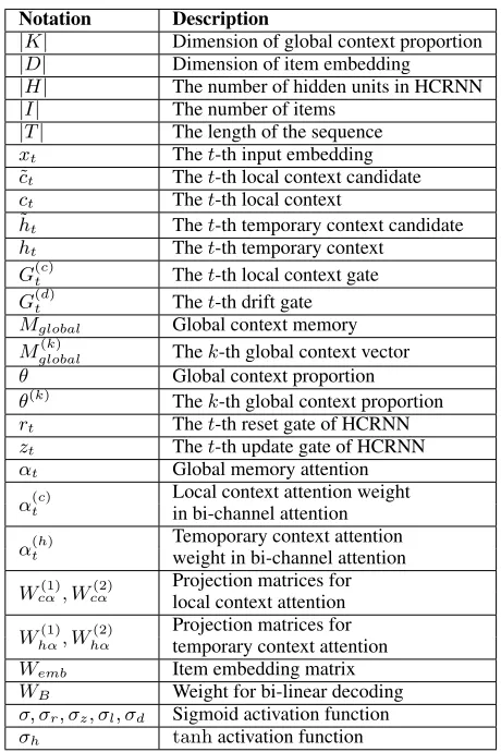
As shown in Figure 1, it is easy to capture the interest drift of the user with a hierarchical context. In other words, we defined theinterest drift assumptionas “if the user’s lo-cal context (for sub-sequence) and the current item are very different, the user’s temporary interest drift occurs.” We pro-posed a new gate structure to incorporate this assumption ef-fectively. As we propose a modified RNN cell and its outputs with different semantics, we also suggest a modified atten-tion mechanism that is complementary to the proposed cell structure. As the global context becomes a static context, the dynamic context becomes the local and the temporary con-texts. Therefore, the attention mechanism will be bi-channel with the local and the temporary contexts, so we named it as thebi-channel attention. By the combination of the HCRNN cells, the attention weight with the local context is concen-trated on the recent history, and the attention weight with temporary context is distributed to the relatively far history. We have presented an overall structure of HCRNN and bi-channel attention in Figure 2.

Figure 2: Overall HCRNN and Bi-channel attention struc-tures. Each different color boxes of theθ is the proportion ofk-th global context vector,θ(k)_{. Each row of the}_M

global

is thek-th global context vector,M_global(k) . Same color of box

inθand row inM_global(k) mean the same global context.

Preliminary

Cell Structure of Recurrent Neural Networks

LSTM LSTM is a de facto standard of RNNs by enabling the learning from the long-term dependency. A variant of LSTM, or LSTM with peephole connection (Gers, Schrau-dolph, and Schmidhuber 2002), is a typical LSTM struc-ture with emphasis on the modified gating mechanism by accepting the input from the cell state, and LSTM with peephole are used in previous studies (Zhu et al. 2017; Neil, Pfeiffer, and Liu 2016). The below is the specifications of LSTM with peephole with formulas.

it=σi(xtWxi+ht−1Whi+ct−1wci+bi) (1)

ft=σf(xtWxf+ht−1Whf+ct−1wcf +bf) (2)

e

ct=xtWxc+ht−1Whc+bc (3)

ct=ftct−1+itσc(ect) (4)

ot=σo(xtWxo+ht−1Who+ctwco+bo) (5)

ht=otσh(ct) (6)

Here, it should be noted that Eq. 6 generates the hidden variable of LSTM, which we consider a temporary context in HCRNN. Eq. 6 does not have any component ofht−1and

it means the high dependency ofht onct. This treatment of connection is hard to consider the semantically different context between the local and the temporary context at the same time.

(3)

GRU GRU is a simplified version of LSTM with fewer parameters while GRU still supports learning from the long-term dependency. GRU replace cell state (ct) and hidden state(ht)in LSTM with one hidden state(ht). The below is the specification of GRU.

zt=σz(xtWxz+ht−1Whz+bz) (7)

rt=σr(xtWxr+ht−1Whr+br) (8)

e

ht= (rtht−1)Whh+xtWxh+bh (9)

ht= (1−zt)ht−1+ztσh(eht) (10)

The enabler of GRU mechanism is Eq. 7 and 8. Hence, when we seek a new gating mechanism to separate the gen-eration of contexts, we were motivated by adopting such condensed gating mechanisms because HCRNN will in-evitably increase the number of trained parameters.

Attention on Recurrent Neural Networks

An RNN representing a context up to the present with a fixed length vector suffers from long-term dependency con-siderations. For that reason, (Bahdanau, Cho, and Bengio 2015) proposed an attention mechanism to retrieve the in-formation needed at present among the past inin-formation. The RNN attention mechanism is usually based only on the hidden state of an encoder (h) and decoder (s) of the RNN. αij = exp(eij)/PT_k₌₁exp(eik) is the attention weight at a point j in time i, and αij is determined by

eij =vTaσ(Wasi−1+Uahj). We were motivated by adopt-ing such a hidden state, h, based attention algorithm be-cause consideration of long-term dependency is important for the sequential recommendation. Besides, in recommen-dation tasks where user interest drifts frequently occur, it is also important to consider the recent user history. For this reason, we have also adopted the local context,c, based at-tention to account for the recent history in the sub-sequence.

Methodology

This paper introduces HCRNN-1, HCRNN-2, HCRNN-3, and bi-channel attention. First, we will explain the overall structure of HCRNN, followed by a detailed modeling of HCRNN and bi-channel attention in order.

Hierarchical Context Recurrent Neural Network

We propose HCRNN, a modification of the RNN structure, to model three hierarchical contexts optimized for recom-mendations, which we describe in this section.

Overall Structure We summarize the overall structure of HCRNN cell at three points. First,htof LSTM, which cor-responds to the temporary context in HCRNN, is generated by thect, which corresponds to the local context in HCRNN. This generation in LSTM indicates that the temporary con-text is directly influenced by the current cell state,ct, while HCRNN has no such direct influence to the temporary con-text, as discussed inintroductionsection. Hence, the gener-ation of the temporary context in HCRNN is detached from

Notation Description

|K| Dimension of global context proportion

|D| Dimension of item embedding

|H| The number of hidden units in HCRNN

|I| The number of items

|T| The length of the sequence

xt Thet-th input embedding ˜

ct Thet-th local context candidate

ct Thet-th local context ˜

ht Thet-th temporary context candidate

ht Thet-th temporary context

G(tc) Thet-th local context gate

G(td) Thet-th drift gate

Mglobal Global context memory

M_global(k) Thek-th global context vector

θ Global context proportion

θ(k) Thek-th global context proportion

rt Thet-th reset gate of HCRNN

zt Thet-th update gate of HCRNN

αt Global memory attention

α(tc)

Local context attention weight in bi-channel attention

α(th)

Temoporary context attention weight in bi-channel attention

Wcα(1), W

(2)

cα

Projection matrices for local context attention

W_hα(1), W_hα(2) Projection matrices for_{temporary context attention}

Wemb Item embedding matrix

WB Weight for bi-linear decoding

σ, σr, σz, σl, σd Sigmoid activation function

σh tanhactivation function

Table 1: The description for the notation in this paper.

the local context, and the local context and temporary con-text has the connection through the gating mechanism. This makes the creation of temporary contexts more flexible and captures instantaneous interest drift.

Second, we introduce a new static context in the RNN struc-ture as the global context. HCRNN models the global con-text as two latent variables ofMglobal andθ. Global

con-text memoryMglobalcontains global context vectorMglobal(k) for each global context componentk.θis the global context proportion, which means the weight of each global context in the sequence. In other words,θ(k)_{is the proportion of}

(4)

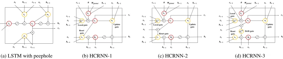
(a) LSTM with peephole (b) HCRNN-1 (c) HCRNN-2 (d) HCRNN-3

Figure 3: HCRNN structure and LSTM with peephole structure. Unlike LSTM, the creation of temporary contexts, ht, in HCRNN is separated from local contexts,ct. Also, the and the local contexts,ct, are designed to be influenced by the item embedding,xt, only through the gate or attention structure. For this reason, the local context can have a more abstract context than a temporary context. Besides, we propose a new gate structure to incorporate the interest drift assumption relatively strongly to HCRNN-1, HCRNN-2, and HCRNN-3.

context by reflecting the global context proportion at each timestep. For example, if most of the items in a sequence are action movies, the HCRNN is trained to have a high prob-ability in generating a local context associated with the ac-tion movie. 3) When the global context is imported into the current local context in Eq. 13,14, we utilize the temporary context,ht, so a local context, ct is adapted to the global context influenced by the temporary context. The HCRNN cell in Figure 2 illustrate this hierarchical context generation ofMglobal,θ,ct, andht.

Third, we designed the gating structure to reflect the in-terest drift assumption by hierarchical contexts. Figure 1 il-lustrates an occurrence of interest drifts when a user selects an item different from the local context. To reflect this inter-est drift assumption, we modified the reset gate in HCRNN-2 as shown in Eq. HCRNN-21. Furthermore, HCRNN-3 has a drift gate,G(td) in Eq. 22, with only local context (ct) and cur-rent item embedding (xt) while the reset gate is influenced by the previous temporary context (ht−1), the local context,

and the item embedding, jointly.G(td)emphasizes the reset initiated only by the interest drift. Figure 3 shows the overall structure of LSTM and HCRNN-1,2,3 structure.

HCRNN-1 The first version of HCRNN introduces the global contexts and the modified structure from the LSTM cell. First, as we introduced in the previous section, the global context consists of the global context proportion,θ, and global context memory, Mglobal. Here,θ is similar to the topic proportion in general topic models, such as LDA (Blei, Ng, and Jordan 2003), and our model is designed by following the TopicRNN (Dieng et al. 2017). However, un-like TopicRNN, we introduceMglobaldesigned as a memory network holding the abstract information, represented as an embedding of each topic, or a global context in the recom-mendation domain.

The modification consists of two phases. First, to model the local context candidate_ect, we modeled the degree,αt, to which we should consider for each global context vector, M_global(k) , at the current time step.αtis obtained from the at-tention mechanism, which is different from the bi-channel attention in Bi-channel Attention and Prediction section,

based on the previous temporary contextht−1, Mglobaland

θin Eq. 13. This attention ofαtis an attention mechanism within the HCRNN cell, yet the bi-channel attention is at-tention outside of the HCRNN cell sequence. Because αt is computed with the temporary context of ht−1, the local

context candidate, _ect, can fluctuate temporarily. To handle this fluctuation, we formulate a local gate,G(tc)in Eq. 15, 16. The local gateG(tc), helps local context to change more stable, different with temporary context.

The second phase is modeling the temporary context, ht, with the current input, xt, and the previous tempo-rary context,ht−1. The temporary context does not directly

come from the local context ofctand the global context of

θ, Mglobal. However, the reset gate ofrtuses the local and the temporary contexts to reset the components of the tem-porary context. Additionally, the update gate ofztcontrols the update with the current input, the local and the tempo-rary contexts. This structure allows the tempotempo-rary context to focus more on the current input, unlike the local context.

e

θ∼q(θe) =N(eθ;µ(x1:T),diag(σ2(x1:T))) (11)

θ∼softmax(eθ) (12)

α(tk)=softmax(v T

θσ(ht−1Whα+ (θ(k)M

(k)

global)Wθα)) (13)

ect=

K

X

k=1

α(tk)M

(k)

global (14)

G(tc)=σl(xtWxl+ht−1Whl+ct−1Wcl+bl) (15)

ct= (1−G

(c)

t )ct−1+Gt(c)ect (16)

zt=σz(xtWxz+ht−1Whz+ctWcz+bz) (17)

rt=σr(xtWxr+ht−1Whr+ctWcr+br) (18)

eht= (rtht−1)Whh+xtWxh+bh (19)

ht= (1−zt)ht−1+ztσh(eht) (20)

µandσ2 _{for the normal distribution denote the output of}

(5)

Table 1 denotes the notation for HCRNN.

HCRNN-2 After we suggest HCRNN-1, we update the generation of temporary contexts,ht, by modifying the reset gate with the local context,ct; the temporary context,ht; and the input,xt. Under the interest drift assumption, the interest drift can be identified if the local context and the current in-put are very different. If the interest drift occurred, we need to further update the temporary context,ht, by reducing the information fromht−1, than the case without the drift. Thus,

the comparison between the local context and the current in-put is necessary to gauge the necessity ofht−1. Finally, we

substitute Eq. 18 with Eq. 21 as the below.

rt=σr(xtWxr+ht−1Whr+ (xtct)Wd+br)

s.t.Wd≥0 (21)

Eq. 21 design the reset gate, so that the rt becomes small as the element-wise product between ct and xt decreases because of interest drift. This similarity magnitude needs to be scaled and regularized, so we multiply a constraintWd≥

0. Also, we used a projection operator (Rakhlin, Shamir, and Sridharan 2012) to handle the constraint.

HCRNN-3 The reset gate in HCRNN-2 reflects the inter-est drift assumption on updating the temporary context. This update in HCRNN-2 requiresxt,ht−1, andctto be mixed to generate the signal of the reset gate. The suggested update linearly models the relevance between the local context,ct, and the current input,xt. However, the linear activation from the element-wise product may not embody the binary nature of the temporary drift. Hence, we add a sigmoid activation on top of the element-wise product, which eventually be-comes an independent gate,G(td), to model the interest drift. Since the sigmoid function outputs a value between 0 and 1, the reset gate of HCRNN-2 in Eq. 21 can have a value be-tween 0 and 1 theoretically. However, the sigmoid function is not sharp, and it makes the most LSTM forget gate values (similar to reset gate in GRU) are experimentally located in the middle state (0.5) (Li et al. 2018). In fact, in our experi-ments, the reset gate,rtin Eq. 21 is on the average 0.47 (± 0.03) on the CiteULike dataset. To make the temporary con-text focus onxt, the value of gate multiplied byht−1in Eq.

19 need to be smaller. We model the new interest drift gate (Eq. 22) and use the product of Eq. 22 and 23 in Eq. 24. The product of Eq. 22 and 23 has a value of 0.29 (_±0.021) on average, and it is 38.2% smaller than that of Eq. 21.

G(td)=σd((xtct)Wd+bd) s.t.Wd≥0 (22)

rt=σr(xtWxr+ht−1Whr+br) (23)

e

ht= (rt(G(td)ht−1))Whh+xtWxh+bh (24)

Eq. 22, 23 lets the temporary context be more affected by the current input when the temporary drift is captured by the drift gate,G(td).

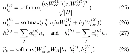
Bi-Channel Attention and Prediction

As mentioned in the Introduction, it is important to learn from both long-term dependency and recent interest in a

se-quential recommendation. One common technique to em-phasize the long-term dependency is an attention mecha-nism, but we introduce modified attention given a HCRNN cell structure because of its hierarchical contexts. To ex-ploit the hierarchical contexts of HCRNN, we implement the complementary bi-channel attention as the local context at-tention,α(tc); and the temporary context attentionα

(h)

t . Both α(tc) andα

(h)

t needs to result in a higher attention weight if two compared context vectors are similar. α(th) is modeled as a conventional linear sum based alignment function, so the training on the weight parameter can select which to attend in the temporary context. The projection ma-trices forα(_th)areW_hα(1), W_hα(2)which are both_|H_|×|H_| ma-trix. Besides, we implemented the scaled dot-product based attention function (Vaswani et al. 2017) forα(tc)because the dot-product will maximize the attention with the same local context vectors. This modeling will produce a stronger at-tention weight to the items in the similar sub-sequence. The projection matrices forα(tc)areW

(1)

cα, Wcα(2)which are both

|D_{| × |}H_|matrix.

We used a concatenation ofht,h(tc), andh

(h)

t for the ap-propriate item prediction with a bi-linear decoding scheme following NARM as in Eq. 28.Wembis an item embedding, andWB is a weight for bi-linear decoding. We calculated the prediction-related loss through cross-entropy.

α(_tjc)=softmax((ctW

(1)

cα)(cjWcα(2))T

p

|H| ) (25)

α(tjh)=softmax(vhTσ(htW_hα(1)+hjW_hα(2))) (26)

h(tc)=

X

j

α(tjc)hj and h(th)=

X

j

α(tjh)hj (27)

b

yt=softmax(WembT WB[ht, h(tc), h

(h)

t ]) (28)

Model Inference

While training the local and the temporary contexts relies on the gradient method with a deterministic learning, HCRNN includes the global context which follows the topic proba-bilistic model, such as LDA, VAE, and GSM (Kingma and Welling 2014; Miao, Grefenstette, and Blunsom 2017). This generative modeling requires a maximization on the log-marginal likelihood of Eq. 29, so we utilize the variational inference by optimizing the evidence lower bound (ELBO) of Eq. 30 (Jordan et al. 1999).

logp(y1:T|c1:T, h1:T) = log

Z

p(θe) Y

t=1

p(yt|θ, ce t, ht)dθe (29)

≥

T

X

t=1

E_q₍

e

θ)[logp(yt|θ, ce t, ht)]−KL[(q(θe)||p(θe))] (30)

(6)

q(eθ) =N(z;µ(x1:T),diag(σ2(x1:T))) (31)

µ(x1:T) =Wq(1)f(x1:T) +b(1)q (32)

logσ(x1:T) =Wq(2)f(x1:T) +b(2)q (33)

After the inference onµandlogσ, the sampledθeis used

as the global context after turning it intoθby the softmax function. Our HCRNN source code is available at https:// github.com/gtshs2/HCRNN.

Experimental Result

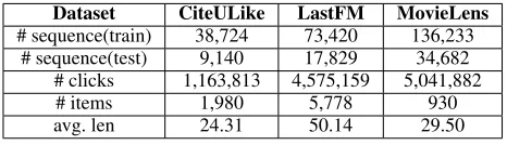
Datasets For the performance evaluation, we used three publicly available datasets: CiteULike, LastFM, and Movie-Lens1. We aim at modeling a long user history, so we re-moved sequences whose length is less than 10. Besides, we removed the items that exist only in the test set, and the items that appeared less than 50/50/25 times in three datasets re-spectively. We performed cross-validation by assigning 10% of the randomly chosen train set as the validation set. We also followed the data augmentation method as proposed in NARM (Li et al. 2017) and improved GRU4REC (Tan, Xu, and Liu 2016). The data augmentation techniques can enhance the performance by reducing the overfitting. Ta-ble 2 summarizes the descriptive statistics of preprocessed datasets.

Dataset CiteULike LastFM MovieLens

# sequence(train) 38,724 73,420 136,233 # sequence(test) 9,140 17,829 34,682

# clicks 1,163,813 4,575,159 5,041,882 # items 1,980 5,778 930 avg. len 24.31 50.14 29.50

Table 2: Statistics of evaluation datasets.

Baselines We compared HCRNN with the below eight baselines.

• POPexploits the frequency of items in the training set. It always recommends items that appear most often in the training set.

• SPOP is Similar to POP, S-POP also exploits the fre-quency, but it recommends items that appear most often in the current sequence.

• Item-KNN (Davidson et al. 2010; Linden, Smith, and York 2003) recommends items based on the co-occurrence number of item pairs, and Item-KNN inter-prets the co-occurrence as a similarity. The model recom-mends similar items only in the same sequence.

• BPR-MF (Rendle et al. 2009) is a model representing a group of models with matrix factorization (MF) and Bayesian personalized ranking loss (BPR). By introduc-ing the rankintroduc-ing loss, BPR-MF shows a better performance than a typical MF in the recommendation.

1

We converted it into a binary implicit rating by activating only the maximum rating.

• GRU4REC (Hidasi et al. 2016) is a sequential model with GRUs for the recommendation. This model adopts a session parallel batch and a loss function such as Cross-Entropy, TOP1, and BPR.

• LSTM4RECis our version of a GRU4REC variant with LSTM.

• NARM(Li et al. 2017) is a model based on GRU4REC with an attention to consider the long-term dependency. Besides, it adopts an efficient bi-linear loss function to improve the performance with fewer parameters.

• STAMP(Liu et al. 2018) considers both current interest and general interest of users. In particular, STAMP used an additional neural network for the current input only to model the user’s current interest. Also, it proposes a tri-linear loss function.

Experiment Settings For fair performance comparisons, we set the batch size (512), the item embedding (100), the RNN hidden dimension (100), the input dropout (0.25), the output layer dropout (0.5), the optimizer (Adam), and the learning rate (0.001)2as shown in NARM (Li et al. 2017).

Quantitative Performance Evaluation

Table 3 shows the performance of the baselines and HCRNN with two measurements ofrecallat K (R@K) andmean re-ciprocal rankingat K (M@K), which are widely used in the sequential recommendation. We varied K by 3 and 20. The experiments on HCRNN has an ablation study variation of HCRNN-1, HCRNN-2, HCRNN-3, and HCRNN-3 with bi-channel attentions (HCRNN-3+Bi). The quantitative evalu-ation indicates that the varievalu-ations of HCRNN have signifi-cant performance improvements in all data and metrics. Par-ticularly, HCRNN-3 with the bi-channel attentions always exhibits the best performance. Additionally, the better per-formance of HCRNN over NARM, which also has a con-text modeling, may suggest the need for hierarchical concon-text modeling in recommendations. Moreover, HCRNN shows the best result compared to the RNN based recommenda-tions, i.e., NARM, GRU4REC, and LSTM4REC, so the modified HCRNN cell may have contributed to the perfor-mance improvements. As HCRNN-3 with drift gate,G(td), shows better results than HCRNN-1 and HCRNN-2, our in-terest drift assumption may be experimentally justifiable. As HCRNN-3+Bi is the best case, we justify that bi-channel attention with hierarchical contexts may improve the per-formance experimentally. Finally, NARM with RNN and at-tention shows better performance than STAMP with a feed-forward neural network. This demonstrates the importance of sequential modeling in recommendations with long se-quences.

Qualitative Analysis

From the sensitivity perspective, the global context is un-likely to change given a single item. The local context should

2

(7)

CiteULike LastFM MovieLens

R@3 R@20 M@3 M@20 R@3 R@20 M@3 M@20 R@3 R@20 M@3 M@20 POP 1.44 5.78 0.92 1.44 0.37 1.99 0.34 0.51 2.43 12.51 1.54 2.65 S-POP 1.26 4.99 0.79 1.23 0.87 3.65 0.55 0.87 2.27 12.23 1.42 2.52 Item-KNN 0.00 6.90 0.00 4.79 0.00 11.59 0.00 8.00 0.00 6.32 0.00 4.28 BPR-MF 0.49 3.15 0.27 0.60 0.82 2.15 0.59 0.73 1.69 8.93 1.07 1.91 LSTM4REC 7.07 23.33 4.93 6.82 15.29 24.75 12.68 13.95 8.52 32.80 5.63 8.45 GRU4REC 8.37 24.19 5.98 7.86 18.29 26.46 15.85 16.95 8.50 32.74 5.60 8.42 NARM 7.81 24.82 5.40 7.41 18.30 33.60 13.12 15.25 9.14 33.42 6.09 8.93 STAMP 5.09 21.93 3.25 5.22 9.29 19.84 6.62 8.01 3.95 20.52 2.65 4.47 HCRNN- 1 8.60 25.36 6.18 8.16 20.67* _34.40* _15.77 _17.68* _9.23 _33.78* _6.13 _9.00

HCRNN- 2 8.83 25.10 6.41* _8.38* _20.78* _34.14* _16.20 _18.08* _9.22 _33.76* _6.14 _9.01

HCRNN- 3 9.21* 25.42* 6.65* 8.61* 21.39* 34.72* 16.66* 18.52* 9.38* 33.67* 6.23* 9.08* HCRNN-3 + Bi 9.33* 25.81* 6.74* 8.70* 21.90* 34.80* 17.33* 19.12* 9.53* 33.83* 6.38* 9.21*

Improvement(%) 11.47 3.99 12.71 10.69 19.67 3.57 9.34 12.80 4.27 1.23 4.76 3.14

Table 3: Performance evaluation of the proposed models. The boldface indicates the best result among our models and the underline indicates the best result among the baselines.P∗_<₀_.₀₅_(Student’s_t_-test)

change when the item selection is dissimilar to the previ-ous selection, but if the selections are similar, the local con-text does not change much by Eq. 13-16. The temporary context likely changes for each selected item to represent the current interest and the temporary context significantly changes when the genre transition happens. Because of the two gating structure of Eq. 24 modeling, the average amount of change in the temporary context is more significant than that of the local context as our assumption and expectation. Experimentally, with CiteULike, the temporary context, h, changes 0.278(_±0.037) on average at every timestep, and the local context, c, changes by 0.005(_±0.024) on average.

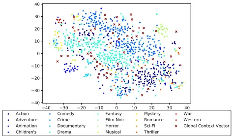
Context Embedding This study models the hierarchical context, global context memory (Mglobal), local context (ct), and the temporary context (ht). The local context is gener-ated by the global context memory, and the temporary con-text is generated by the previous temporary concon-text and the current item embedding (xt). The first analysis is visualizing the global context memory (Mglobal) and the item embed-ding (xt), to verify the quality of inputs to the construction on the local context (ct) and the temporary context (ht). Fig-ure 4 is the joint visualization of the item and the global con-text memory. The item embeddings are coherently organized as a cohesive cluster with the same genre, and the global context memory covers most of the area that the item em-beddings are dispersed. Given the item and the global con-text memory, we calculated the cosine similarity, and Table 4 enumerates the most aligned items with a specific global context vector in the global context memory.

Gate Analysis HCRNN is a model to capture the user’s in-terest drift with hierarchical context and drift gateG(td). For the comparison of HCRNN and NARM gate structures, we definerHCRN N

t and rtN ARM as the HCRNN and NARM

reset gates, respectively. In order to incorporate the interest drift assumption, we designed the value ofrHCRN N

t G

(d)

t gate applied toht−1to be smaller when updatingehtin Eq.

40 30 20 10 0 10 20 30 40

Action Adventure Animation Children's

Comedy Crime Documentary Drama

Fantasy Film-Noir Horror Musical

Mystery Romance Sci-Fi Thriller

War Western Global Context Vector

Figure 4: Item embedding and global context vector, Mglobal(k) , visualization with tSNE(van der Maaten and Hin-ton 2008). Item embedding is interpretable with genre, and global context vector cover the most of the items.

24 if interest drift occurred. Figure 5 represents the gate value when the user clicks the same genre of an item as the previous step and when the user does not. The x-axis in Fig-ure 5a represents the number of consecutive items which has the same genre until the right before timestep. In general, if the genre of the current input is different with previous items,rHCRN Nt G

(d)

t has a smaller value compared to the opposite situation. Besides, when a user clicked the same genre of items consecutively, and instantly clicks a differ-ent genre of items, the value ofrHCRN N

t G

(d)

t becomes smaller.

(8)

histo-Genre Movie Title

M_global(6) Animation Pinocchio, Yellow Submarine, Snow White and the Seven Dwarfs

Mglobal(19) Action

Star Trek: Generations, Predator, Butch Cassidy and the Sundance Kid

M_global(31) Horror Scream, An American Werewolf in London, Dracula

Table 4: Interpretation of global context vector. We listed the items (movie title) close to each global context vector.

0 5 10 15 20 25 30

Number of times with similar genre 0.240

0.245 0.250 0.255 0.260

Average

value

rHCRN Nt G(d)

t with similar genre

rHCRN N

t G(d)

t with different genre

(a) Average value ofrHCRN Nt

G(td) gate after appearing items

with similar genre consecu-tively.

√ √

(case 1)

(case 2)

Time

(b) Gate heatmap for a user his-tory as an example. We mark “check” when the genre of item changes.

Figure 5: HCRNN takes a large value ofrHCRN N

t G

(d)

t if the current input of item has similar genre with previous input of item. In the opposite case, HCRNN grasps the user’s interest drift and changesrHCRN N

t G

(d)

t to smaller.

2 4 6 8 10 12 14 16 18 ∆t

0.00 0.05 0.10 0.15 0.20

A

ttention

w

eight

αNARM

t in NARM

α(c)

tin bi-channel attention α(h)

t in bi-channel attention

(a) Averaged attention weight over time difference.∆tmeans a time difference between prediction time step and the timestep of the previous user history.

( )

(case 1)

(case 2)

Time

(b) Attention heatmap for a user history. The first row of each case is an attention weight in NARM, and the two be-low are our bi-channel attention weights.

Figure 6: Temporary context based attention, α(th), in HCRNN is spread over a long period relatively. Local con-text based attention,α(tc), in HCRNN has a large value on recent user records.

ries. NARM has a single attention mechanism, so NARM at-tention weight,αN ARM

t , cannot differentiate the attentions on the local and the temporary contexts. However, the bi-channel attentions distinguishes the attentions for the sub-sequence continuation,α(tc); and for the temporary transi-tions,α(th). Figure 6a and 6b indicates thatα

(c)

t focuses on the neighbor attention to check the continuation; and that α(th) spreads out through the whole sequence to check the similar temporary transition.

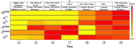
Figure 7: Attention, gate value in NARM and HCRNN, and the change of context value in HCRNN overtime. The drift gateG(td=17) in HCRNN captured the temporary interest drift

Case Study Figure 7 shows the attention weights, and the gate values for selected user history. In Figure 7, the top three rows represent the attention weights comparing NARM and HCRNN. The bi-channel attentions of HCRNN results in two rows of attentions. The attention of local contexts, α(tc), focuses on recent history, and the attention of temporary contexts, α(th), considers relatively far his-tory. These mean that α(tc) emphasizes belonging to the same sub-sequence, andα(th) tries to find the similar tran-sition throughout the entire history. In particular,α(_th₌₁₅) has

a relatively high attention weight compared to α(_tc₌₁₅) and αN ARM

t=15 . The rational behind this temporary high attention

originates from the same genre of the item entered as input at the last timestep,t= 20, whose genre is Romance.

After we observe the attention weights, we observe the gate values, which are rN ARM

t , G

(d)

t , and rtHCRN N, to verify that the gate operates as we expected. We observed thatG(td=17) has a relatively small value. This small value is

caused by the selection of items disaligned to the previous sub-sequence att= 16. This phenomenon demonstrates that G(td)can capture the interest drift to reset the temporary con-text to accept further information from the current item em-bedding ofxt, as designed in Eq. 22. AsG(td)is controlled by the local context, the discontinuation of genre matters inG(td). However,rHCRN Nt , which also controls the reset of the temporary context in Eq. 23, is not activated because rHCRN N

t only takes the temporary context as the inputs, so the discontinuation does not matter inrHCRN N

t . This ratio-nale applies torN ARM

t , as well. On the contrast, the user history has the same genre att = 18,19,20, soG(td) also keeps high gate values to prevent the reset on the temporary context.

Conclusion

(9)

memory network to contain the abstract information for the global and the local contexts. We also propose the new gate mechanism to incorporate the interest drift assumption. To support HCRNN with hierarchical contexts, we propose bi-channel attentions to account for both long-term dependency and recent interest in the long user history.

Acknowledgments. This research was supported by Basic Science Research Program through the National Research Foundation of Korea (NRF) funded by the Ministry of Edu-cation (NRF-2018R1C1B6008652).

References

Bahdanau, D.; Cho, K.; and Bengio, Y. 2015. Neural ma-chine translation by jointly learning to align and translate. International Conference on Learning Representations.

Blei, D. M.; Ng, A. Y.; and Jordan, M. I. 2003. Latent dirichlet allocation. Journal of machine Learning research 3(Jan):993–1022.

Cho, K.; Van Merri¨enboer, B.; Gulcehre, C.; Bahdanau, D.; Bougares, F.; Schwenk, H.; and Bengio, Y. 2014. Learning phrase representations using RNN encoder-decoder for statistical machine translation. arXiv preprint arXiv:1406.1078.

Davidson, J.; Liebald, B.; Liu, J.; Nandy, P.; Van Vleet, T.; Gargi, U.; Gupta, S.; He, Y.; Lambert, M.; and Livingston, B. 2010. The YouTube video recommendation system. In Proceedings of the fourth ACM conference on Recommender systems, 293–296. ACM.

Dieng, A. B.; Wang, C.; Gao, J.; and Paisley, J. 2017. Top-icrnn: A recurrent neural network with long-range semantic dependency. International Conference on Learning Repre-sentations.

Gers, F. A.; Schraudolph, N. N.; and Schmidhuber, J. 2002. Learning precise timing with LSTM recurrent networks. Journal of machine learning research3(Aug):115–143.

Hidasi, B.; Karatzoglou, A.; Baltrunas, L.; and Tikk, D. 2016. Session-based recommendations with recurrent neural networks. International Conference on Learning Represen-tations.

Jordan, M. I.; Ghahramani, Z.; Jaakkola, T. S.; and Saul, L. K. 1999. An introduction to variational methods for graphical models. Machine learning37(2):183–233.

Kingma, D. P., and Welling, M. 2014. Auto-encoding vari-ational bayes.International Conference on Learning Repre-sentations.

Lau, J. H.; Baldwin, T.; and Cohn, T. 2017. Topically driven neural language model.arXiv preprint arXiv:1704.08012.

Li, J.; Ren, P.; Chen, Z.; Ren, Z.; Lian, T.; and Ma, J. 2017. Neural attentive session-based recommendation. In Pro-ceedings of the 2017 ACM on Conference on Information and Knowledge Management, 1419–1428. ACM.

Li, Z.; He, D.; Tian, F.; Chen, W.; Qin, T.; Wang, L.; and Liu, T.-Y. 2018. Towards binary-valued gates for robust lstm training.arXiv preprint arXiv:1806.02988.

Linden, G.; Smith, B.; and York, J. 2003. Amazon. com rec-ommendations: Item-to-item collaborative filtering. IEEE Internet computing(1):76–80.

Liu, Q.; Zeng, Y.; Mokhosi, R.; and Zhang, H. 2018. STAMP: Short-Term Attention/Memory Priority Model for Session-based Recommendation. In Proceedings of the 24th ACM SIGKDD International Conference on Knowl-edge Discovery & Data Mining, 1831–1839. ACM. Miao, Y.; Grefenstette, E.; and Blunsom, P. 2017. Discov-ering discrete latent topics with neural variational inference. International Conference on Machine Learning.

Neil, D.; Pfeiffer, M.; and Liu, S.-C. 2016. Phased lstm: Ac-celerating recurrent network training for long or event-based sequences. InAdvances in Neural Information Processing Systems, 3882–3890.

Rakhlin, A.; Shamir, O.; and Sridharan, K. 2012. Making gradient descent optimal for strongly convex stochastic op-timization. International Conference on Machine Learning. Rendle, S.; Freudenthaler, C.; Gantner, Z.; and Schmidt-Thieme, L. 2009. BPR: Bayesian personalized ranking from implicit feedback. InProceedings of the twenty-fifth conference on uncertainty in artificial intelligence, 452–461. AUAI Press.

Smirnova, E., and Vasile, F. 2017. Contextual sequence modeling for recommendation with recurrent neural net-works. InProceedings of the 2nd Workshop on Deep Learn-ing for Recommender Systems, 2–9. ACM.

Sukhbaatar, S.; Weston, J.; Fergus, R.; et al. 2015. End-to-end memory networks. InAdvances in neural information processing systems, 2440–2448.

Tan, Y. K.; Xu, X.; and Liu, Y. 2016. Improved recur-rent neural networks for session-based recommendations. In Proceedings of the 1st Workshop on Deep Learning for Rec-ommender Systems, 17–22. ACM.

van der Maaten, L., and Hinton, G. 2008. Visualizing data using t-SNE. Journal of machine learning research 9(Nov):2579–2605.

Vaswani, A.; Shazeer, N.; Parmar, N.; Uszkoreit, J.; Jones, L.; Gomez, A. N.; Kaiser, Ł.; and Polosukhin, I. 2017. At-tention is all you need. InAdvances in Neural Information Processing Systems, 5998–6008.

Wu, C.-Y.; Ahmed, A.; Beutel, A.; Smola, A. J.; and Jing, H. 2017. Recurrent recommender networks. InProceedings of the tenth ACM international conference on web search and data mining, 495–503. ACM.

Yin, H.; Zhou, X.; Cui, B.; Wang, H.; Zheng, K.; and Nguyen, Q. V. H. 2016. Adapting to user interest drift for poi recommendation.IEEE Transactions on Knowledge and Data Engineering28(10):2566–2581.