C. W. Robbins A and W. S. Meyer B
A USDA-ARS, Soil and Water Management Research Unit, 3793 N. 3600 E., Kimberly ID, 83341.
B Division of Water Resources, CSIRO, Griffith, N.S.W. 2680.
Abstract
Currently used soil salinity models do not contain a mechanism for including exchangeable sodium effects on soil pH. A method is needed that allows pH calculation from the sodium adsorption ratio (SAR) or exchangeable sodium percentage (ESP) and electrical conductivity (EC) data. This study developed a simple method for calculating saturated soil paste and aqueous solution pH from SAR (or ESP) and EC data and compared the results with measured values from a number of soils and subsurface waters. The equation pH - A+{B*(SAR) 1/2 /(1+CEC)I estimated soil pH from EC and SAR or ESP values. When rewritten as: SAR or ESP = l(pH-A)(1+C'EC)/13} 2 , the SAR or ESP was estimated from pH and EC data. By using shallow bore (well) water and soil extract data from the Murray Basin, values were determined for the scalar terms A, B and C. These values differed among subsurface water and soil types, however, the range of each scalar was reasonably small. It was found that a range of at least 2 . 5 pH units in the calibration data was necessary to obtain reliable regression between predicted and measured pH and SAR or ESP values. When these conditions were met, the predicted results were satisfactory. These relationships provide a method for pH calculation in soil salinity models which takes into account soil EC and sodium effects. They also provide a rapid field method to estimate SAR or ESP from easily obtainable EC and pH data. Further research is needed to define the factors that determine the values of A, B and C.
Introduction
Chemistry models and subroutines currently available for predicting lime and gypsum precipitation and dissolution in saline and sodic soils do not take into account the effects of exchangeable sodium nor soil solution electrical conductivity (EC) on soil pH (Tanji and Doneen 1966; Robbins et al. 1980; Suarez 1982). Models using these calculation methods are also restricted to soils containing lime. A more realistic prediction method is needed to include ESP or SAR and EC effects on soil and solution pH in saline and sodic soil models, regardless of whether lime is present or absent.
by using the methods of Rhoades et al. (1989a), or points in the landscape
can be readily monitored with depth by using electrical conductivity probes (Rhoades and van Schilfgaarde 1976). Soil salinity can also be easily and rapidly determined by using saturated soil pastes (Rhoades et al. 1989b) or saturation paste extract (Rhoades 1982) electrical conductivity methods. The method selected for measuring soil pH varies, depending on the purpose for measuring pH. The most widely accepted method for saline and sodic soils is the saturation paste pH, followed by saturation paste extract pH. These procedures are simple and quick, and pHsp data from different soils can be compared without the concern of relative dilution differences among different soil textures (U.S. Salinity Lab. Staff 1954; Tucker and Beatty 1974; Rhoades 1982).
In order to obtain ESP data, considerably more work and expensive laboratory equipment is required, and consequently it is more costly. As a partial solution to this problem, the sodium adsorption ratio (SAR) concept was developed as an alternative approximation to ESP measurement when used for soil extracts, and to predict soil ESP equilibrium from irrigation water quality. Over the range 0-35, SAR and ESP are not significantly different in terms of practical application. At values greater than 35, conversion graphs and equations are available (U.S. Salinity Lab. Staff 1954; Robbins 1984). Both ESP and SAR data are subject to greater analytical error than pHsp or ECe data because more analytical steps are required (at least twenty separate operations on each sample for ESP and seven for SAR). Because of the differences in data gathering costs, pH and EC data are much more likely to be available for a particular site than the ESP or SAR data. However, ESP or SAR values are needed for monitoring exchangeable sodium changes and severity in salt-affected soils.
Fireman and Wadleigh (1951) attempted to predict ESP from pHsp and saturation extract pH, data, using data from 868 soils and linear regression analysis. They concluded that an ESP increase of 20 corresponded to an average increase of 1 pH unit and, that if the pH was 8 . 5, then the ESP would be between 17 and 50 for two thirds of the time. Less than half of the ESP variation could be attributed to pHsp. When they sorted the soil data according to lime and gypsum presence or absence, the relationship between pHsp and ESP improved only slightly. The soil : water extraction ratio used also affected the pH results, with pHsp being the most effective predictor of ESP. Even though they showed that an increase in ESP tended to increase the saturation paste pH, they were unsuccessful in developing a practical relationship for diagnosing the soil Na status from pHsp data alone.
co -0 c V) 41 ....
'V co
• V
u 3,3
OJ
0. -• ••• rd 0.) .n
E
0
3-..., . .0 a
-o E 0 c CO ,••••n CO N E
u co 0 0
E
OJ 111
x
-rc d
• w0 00 -0 at
01 (0
0 V) 0 u
,..,
=
a.3 W^. <
3
..5 in C 0E 0 ..-,0
= eel 144.
0 4-. 0.1 x etE Na 17; o
o d -o 0.
3/3 p 0 0.,
7.5 ra, re; x
rt3 3 Cr, V co
n-n u . 8 13 LL., -6
E- .5 CD 0 u - c
3- ea ea ...,
... . u .
fo 7< ci C
• 43:1-'z w Z O
E 8 ' a= w
a. 3
-= = co E o a) o 7'z to ez:
= (Is ... L. co a
no a -C, , 0.)
•7.. 444. 4. ..X
al ti 0 VI 0) •-• c
c
1
..Y a, cc T.
.•-• 0 3-co .-, - ,,, ea 0.3
-a -0.1
ce i.
(A 0 ‘.."rrl
C
CO %-• ›:.
u ° .."'
1.1.3
ta
±-
a
c
0. (r3 0 .,••• al =
U NN ra ,... ,I) ic FE, (>' 0) • 4,
c a >. .--- m 5 RI .1. .^.. c" E •tA. 4 . 4. 0 ,, a: 3- (3.3
N4-, 1...
a
t N
/V
1- al °i.'t W C
rn 3- 11:3 0 C
0 331 31.3
0) L.
4) 0 C
• L co
ea
•
• u C >,-0
11.1 CO 6. 1.
> tz4 (...)
values less than 4 dS m-1 have been designated as sodic (Seatz and Peterson 1964). Each of these soil categories requires different management methods if successful reclamation is to be achieved.
Combination of these observations leads to hypothesizing a relationship of the form
pH = A + {B*SAR/(1.0+C*EC)}, (1)
where A would be expected to be greater than 5.5. The B term is the SAR
scaling factor and is a function of the relative impact of SAR on pH. The unity term in the denominator keeps the denominator from becoming less than 1 .0, regardless of how small EC might be, and C is the EC effect scaling factor determined by the relative impact of EC on pH.
The purpose of this study was to test the simple pH relationship as a method for estimating soil pH change as a function of EC and SAR changes in soil salinity models and to calibrate the A, B and C coefficients from a variety
of soil extract and subsurface drainage water data. The secondary purpose was to rewrite the relationship in terms of SAR as a function of pH and EC and to test its use as a simple and rapid field estimation method of SAR or ESP from ECe and pHsp or pHe data.
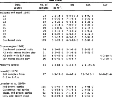
Table 2. Measured EC, pH, SAR and ESP ranges of the water and soil data used in this study
Data source
No. of samples
EC (dS m-1 )
pH SAR ESP
Williams and Ward (1987)
GI 23 0 . 2-18 . 1 6 . 9-10 . 2 1 . 6-99 . 1
G2 14 1 . 6-26 . 4 7 . 1-8 . 5 6-1-26 . 1
G3 18 0 . 4-25-2 6 . 4-8 . 8 1 . 3-25 . 0
L5 26 0 . 1-14-0 7 . 0-9 . 7 1 . 3-25 . 0
C6 19 0 . 3-8 . 6 6 . 6-9-9 1 . 2-18 . 3
C7 29 0 . 3-15 . 1 7 . 3-8-2 1 . 9-9 . 4
C8 18 1 . 0-28 . 2 6 . 9-8-1 1-2-17 . 6
L9 22 0-1-17 . 5 6 . 5-8 . 5 0-6-34 . 2
Combined data 169 0-1-28 . 2 6 . 5-10 . 2 0 . 6-99 . 1
Groenewegen (1961)
Combined data-all soils 24 1 . 2-49 . 6 5 . 1-8 . 6 3 . 3-51 . 7 All soils minus Mallee clay 21 1 . 2-49 . 6 5 . 1-8 . 6 3 . 3-51 . 7
All soils with ESP data 18 4 . 0-49 . 6 5 . 6-8 . 4 4 . 2-39-4
ESP minus Mallee clay 16 4 . 0-49 . 6 5 . 6-8 . 4 4.2-39.4
McIntyre (1980) 64 1 . 3-83-5 5-3-8 . 5 2 . 1-155-6
Loveday (1974)
Soil samples from 17 1 . 9-13 . 6 6 . 4-7-4 15 . 2-20 . 1 14-0-21 . 0 0 . 2 to 5 . 0 m
Loveday et al. (1979)
cr, 0
-J U o¢
2¢ 2
VI
1,1 1,1 ••:1- rn M rn
. . . .
000000000
0 N• CO en — N.
N. el• CO
0 0 0 0
V' 00 •-n
(NI 01 CV I. N. CO CO In In CO NI in in N.
csi
•
0 0• 0• 0 0 0 0 0 0• • • • • • 0 0 0 0• • • •
.4* 0 0 0 0 et 0 cr N. 0 •er
•rt• in 00 1.11 t0 C 0 N. CO
0 (...) C 0 0
1;s' 0• 0• 0• 0 0 0 0 0 0• • • • • • 0000
0"
L.1.2
0
.-••n 0rq 00 ON0 0 0 0 0 •cr ff 1 inin tD 0 0 0 00 (NI •cl•
CO in
• V• 0• N. r•J n n tD• • • • • • O 01. . . . 0 0 0 0 0 0 0 0000
0 rn 0 in 0 N rn 0 V) O CN In rn •zC
• VI• 0• CD CS)
•Ci• O1 M Cs1
• • • • • • tD • (.0 (.0 CO• • • CO (.0 V) CO in ID tD Tr V 7 •cr
< CD . V' CO in ei. . . . • u-) m . . M. . Cri CO CO N.. . . .
vi 0 0 0 0 0 0 0 0 0 0 0 0 0
er •-n In 00 N. CO CO r•J NJ 00 (D
L. • C••I• in• in • CO t-4 .3" • • • 'V • .1"• rn 0 0 0 0 0 0 0 0 0 0000
0 0 0 I./1 0 0 0 0 0 In in LA in
o 00 0••••• Inrn •Cf•-• n rn •••••1 •-n tD 0000t10 ger •1"
• • • • • • • • • ' •
0000
0 0 VI in
O CO CO --CO• • • •
0000
O 0 in
N-CO in in in • • • • t0 (.0 CO CO
Lu
00000000C
0 0000 0 N. er•
tDOON.100)01010 CO O N• CO 0 0 0 •nn1 • • • • • • • • • 0 0 0 0 0 0 0 0 0
0 0 in CO O (N iD h C
'aC • p.--.N10(NICI)0101• • • • • • • • N. N. n N. t.D Lo
— CV CO L.7
(.0 N. 00
U U U
O
aJ Li
tb
Materials and Methods
Soil extract and bore (well) water sample data from five sources were used for this study (Table 1). Prior to using these data, the data set for each soil or water sample was evaluated for consistency by determining the electrical charge balance between cations and anions, and calculating the EC from the cation and anion data by using the exponential method of McNeal et al. (1970). Since there was no way to check pH measurements, pH data were assumed to be correct unless bicarbonate and carbonate concentration data contradicted the pH data (Stumm and Morgan 1970). Individual samples that had a cation-anion imbalance, differences in the calculated and measured EC values of 10% or more, or samples that had questionable pH values, were rejected.
Bore water (Williams and Ward 1987) and saturated soil paste extract (Groenewegen 1961) data sets from central N.S.W. were separately entered into a spread sheet program (Tables 1 and 2). By using equation (1), factors A, and B and C were adjusted by tri g ! and error to minimize the sum of squares difference between the measured and calculated pH values. The initial results were only slightly better than previous attempts to predict ESP from pH data (Fireman and Wadleigh 1951). When the square root of SAR was substituted for SAR, the results improved considerably (Table 3). The relationship then became
pH-A + (V(SAR)1/2/(1+CEC)}. (2)
The success of this exercise suggested that equation (2) could possibly be used to predict pH from EC and SAR in soil salinity models. Equation (2) was then rewritten in terms of SAR:
SAR =((pH-A)(1+CEC)/131 2 . (3)
Equations (2) and (3) were then used with the above two data sets plus two additional soil extract data sets of Loveday (1974) and McIntyre (1980) (Tables 1 and 2) to determine if SAR or ESP could be estimated from EC and pH data as a means of rapidly identifying potentially high SAR bore waters or high ESP soil samples by using the more easily obtainable EC and pH data.
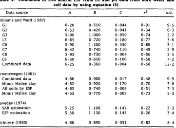
Table 4. Estimation of SAR and/or ESP from EC and pH data from bore water and soil data by using equation (3)
Data source A B C r2 s.d.
Williams and Ward (1987)
G1 6 . 20 0 . 510 0 . 044 0 . 91 9 . 5
G2 6 . 53 0 . 420 0 . 041 0 . 34 6-3
G3 5 . 00 1 . 000 0 . 050 0 . 74 5 . 2
L5 6 . 65 0 . 720 0 . 180 0 . 77 3 . 6
C6 5 . 90 1 . 200 0 . 350 0 . 89 3 . 1
C7 6 . 42 0 . 740 0 . 110 0 . 49 2 . 9
C8 5 . 93 0 . 730 0 . 064 0 . 56 3 . 5
L9 6 . 30 0 . 650 0 . 100 0 . 58 7 . 2
Combined data 6 . 25 0 . 360 0 . 004 0 . 58 12 . 2
Groenewegen (1961)
Combined data 4 . 66 0 . 900 0 . 017 0 . 48 9 . 9
Minus Mallee clay 4 . 62 0 . 920 0 . 170 0 . 70 7 . 8
All soils by ESP 4 . 65 0 . 740 0 . 004 0 . 51 7 . 3
Minus Mallee clay 4 . 63 0 . 770 0 . 005 0 . 73 5 . 3
Loveday (1974)
SAR estimation 5 . 25 1 . 100 0 . 141 0 . 22 3 . 3
ESP estimation 5 . 30 1-130 0 . 143 0 . 26 3 . 4
and individually adjusting A, B or C in a manner that simultaneously minimized the sum of squares difference between measured and predicted pH and SAR or ESP values, using equations (2) and (3) (Table 4). Some data sets only contained SAR data, or data to calculate SAR, while others also contained ESP values or sufficient data to calculate ESP.
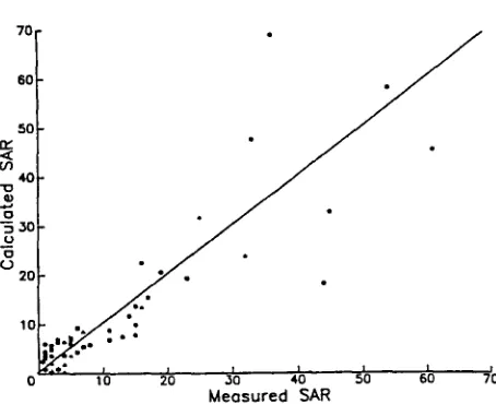
The usefulness of equations (2) and (3) to estimate pH and SAR were then tested by using the extensive data set of Loveday et (1979). These data were collected from 49 sites near Griffith and Leeton, N.S.W., and Kerang, Vic. There were 23 red-brown earth, 9 transitional red-brown earth, 6 calcareous red earth and 11 grey and brown clay profiles, with a total of 300 soil sample data sets. The samples were taken by 0 . 25 m depths down to 1 . 50 m and the deepest samples were from 1-50 to 2 . 00 m. Saturation extracts were made and the pH and EC were measured, while the SAR was calculated from the cation concentrations (Beatty and Loveday 1974). The data from each of the four soil types were randomly divided, by profiles, into two groups. The A, B and C coefficients for equations (2) and (3) were determined as described above on one half of the profiles of each soil type. By using the coefficients thus obtained, the pH and SAR were then estimated for each of the remaining samples for the four soils. The calculated and measured pH and SAR values were then compared. The standard deviation and r 2 values for the pH prediction are given in Table 5, and the results of the SAR predictions are shown in Fig. 1. The combined calculated and measured SAR values for the surface samples (0-0 . 25 m) of each soil profile is also shown in Fig. 2.
Table 5. Estimation of pH and SAR for one set of soil samples by using equations
(2) and (3) and A, B and C values derived from another set of soil samples
Soil A B C pH SAR
r2 s.d. r2 s.d.
Red-brown earths 5 . 86 0 . 630 0 . 052 0 . 68 0 . 4 0 . 72 8 . 2 Calcareous red earths 6 . 13 0 . 560 0 . 055 0 . 52 0 . 4 0 . 61 4 . 5 Trans. red-brown earths 5 . 95 0 . 640 0 . 063 0 . 52 0 . 4 0 . 56 4 . 8 Grey and brown clays 6 . 46 0 . 480 0 . 108 0 . 76 0 . 3 0 . 78 6 . 1
Results and Discussion
By using equation (1) to calculate pH from EC and SAR data from 169 bore water samples (Williams and Ward 1987) and 24 soil samples (Groenewegen 1961), data sets were no better , than the results of Fireman and Wadleigh (1951). When equation (1) was changed by using SARI/2 rather than SAR (equation 2), the r2 values increased and the standard deviation between the measured and estimated pH values decreased (Table 3).
The reasonable success of predicting pH with equation (2) prompted rewriting it in terms of SAR as the unknown (equation 3). By using the two additional data sets of McIntyre (1980) and Loveday (1974), the SAR (and for a few samples ESP) was estimated from EC and pH data by the same method to obtain the constants A, B and C. The standard deviation between predicted
and measured SAR or ESP values was less then 10 and usually less than 8 when data were not combined (Table 4).
When the calculated SAR was plotted against the measured SAR for the independent samples of Loveday et a!. (1979), it was shown that the method
tended to overestimate SAR in the 0-10 region for the red-brown earths (Fig. 1 a)
and the transitional red-brown earths (Fig. lc), while the deviation was more
uniform at higher SAR values for the other two soils (Figs lb and 1d). When
Calculated SAR
U
co
o
co C
C A
so
N 40
0
-0
-5 30 _U
20
10 20 30 40 50
Measured SAR
Fig. 2. Calculated and measured SAR values for the combined surface soil samples (0-0.25 m)
from the data of Loveday et al. (1979). Symbols represent red-brown earths (•), transitional red-brown earths (n), grey and brown clays (A), and calcareous red earths (*).
terms of over- or under-estimation, with the deviation increasing as the SAR increased (Fig. 2).
Examination of the results shown in Figs 1 and 2 show that, if all samples with calculated SAR values greater than 5 are analysed by standard methods, they would have a measured SAR of 10 or greater. If samples with calculated SAR values of 10 or greater are likewise analysed, only two red-brown earths (Fig. 1 a and Fig. 2) with SAR values greater than 15 would have been missed. There would be a limited number of samples selected that would not be necessary to analyse by this selection method. Use of this selection method would reduce the number of samples needing further analysis when the sodium status of the soils was of concern, especially in surface soil samples (Fig. 2). The pH r 2 values for the four soil groups of Loveday et al. (1979) appeared to
be dependent on the measured pH range, even though the standard deviations were 0 . 4 or less. The r 2 values for SAR prediction were larger than those for pH and the SAR standard deviation values were less than 9. In Table 5, the A, B and C values for the first three soils are more alike than those of the grey and brown clays. This may explain why it was necessary to remove the Mallee clay data from the McIntyre (1980) data, in order to obtain reasonable predictions.
All sample sets tested that had pH ranges of 2 . 0 or less pH units failed to give r2 values greater than 0 . 60. Data sets from mixed soil or bore locations also tended to give low r2 values (Tables 3-5). Four bore water sampling area data sets produced r 2 values for SAR and EC greater than 0 . 70 and had pH ranges of 2-7-3 . 7 units. The other four sample area data sets had r2 values of less than 0 . 60 and had pH ranges from 0 . 9 to 2 . 0 units. The combined data for the 169 bore water samples produced an r2 value of 0 . 58 for SAR prediction and • 0 . 61 for pH prediction, even though there was a 3 . 7 pH range of values. The A, B and C values among these samples
came from six different soil profiles with a wide pH range, however, it was
necessary to remove the Mallee clay soil data before a reasonable ESP, SAR or
pH prediction could be achieved. The A, B and C values used for the other
six soils underestimated pH and overestimated SAR for Mallee clay. There was not an obvious reason for the difference. The SAR (and pH which is not shown) prediction from McIntyre's (1980) data was quite good, considering that the samples came from a number of different areas. Good prediction of SAR and pH values for these data was probably due in part to the wide pH range, and the lack of very low EC or pH values. Very low r 2 values were produced from the data of Loveday (1974). The pH range was very narrow, even though the SAR or ESP ranges were quite wide.
Conclusions
Equation (2) provides an empirical method for calculating pH changes in soil models as a function of EC and SAR or ESP changes. This method is more realistic than previous methods, which either held pH constant and calculated CO2 partial pressure as a function of calcium ion activity changes, or held CO2 partial pressure constant and calculated pH as a function of calcium
ion activity and CO 2 partial pressure. The previous calculation methods also required lime to be present. The relationships developed here will cause the soil pH to change as the soil sodium status changes. The magnitude of the change will depend on the soil salinity status, with greater changes at lower EC values and lesser changes at higher EC values. This will more nearly represent what happens in the field. Calcium ion activity can then be calculated as a function of pH, CO 2 partial pressure, lime and/or gypsum precipitation and Ca2+ ion exchange. It would be unwise to predict pH from coefficients derived from data sets that had a pH range of less than 2 . 0 pH units, or to try to extrapolate to pH values outside the range of the calibration data.
Equation (3) provides a potential field method for estimating soil ESP or drainage water SAR from EC and pH data. Portable pH and EC meters are available for solution measurements, and recently developed field methods are now available that allow saturation extract EC to be determined directly from saturation paste EC measurements in the field (Rhoades et al. 1989b). When
suitably calibrated, equation (3) could be used with field pH and EC data to rapidly estimate drainage water or soil sodium status. This would provide a rapid method for identifying samples that should be analysed for ESP or SAR by more rigorous methods, especially under survey-type conditions.
The effects of clay mineralogy, organic matter content, percentage base saturation, lime, gypsum and the solution anions are not taken into consideration by this calculation procedure. The kinds of exchange sites available will influence the pH—ESP interactions. The base saturation percentage or, conversely, the percentage of exchangeable hydrogen and aluminium will influence the pH at a given solution SAR level because they are both held tighter than calcium or magnesium to the exchange sites at low pH. On this basis, the prediction
of pH or SAR at pH values less than about 6 . 5 may not be realistic by
these methods. The ratio of carbonate and bicarbonate to strong acid anions (chloride, sulfate and bisulfate) will influence both pHsp and pHe at a given ESP
in these data to quantify these effects. These factors are at least part of the causes for different A, B and C values among soils and depths in a given soil.
Equations (2) and (3) proposed here need to be further tested on data sets that have been collected and analysed specifically for this purpose. A simple calibration method is also needed which will provide a soil pH range of at least 2 . 0 and preferably 2-5 pH units and an EC range from about 1 to 40 dS m- 1 .
Acknowledgments
The authors wish to acknowledge the help and permission given by Drs J. Loveday, D. S. McIntyre and B. G. Williams to use their original data for this
study. •
References
Beatty, H. J., and Loveday, J. (1974). Soluble cations and anions. In 'Methods for Analysis of Irrigated Soils'. (Ed. J. Loveday.) Comm. Bur. Soils Tech. Commun. No. 54.
Fireman, M., and Wadleigh, C. H. (1951). A statistical study of the relation between pH and the exchangeable-sodium-percentage of western soils. Soil Sci. 71, 273-85.
Groenewegen, H. (1961). Composition of the soluble and exchangeable ions of the salty soils of the Mirrool Irrigation Area (New South Wales). J. Soil Sci. 12, 129-41.
Loveday, J. (1974). Data relating to site of field installation Project CF2-Hydrology and salinity of a deep clay profile. CSIRO Aust. Div. Soils, Tech. Mem. 41/1974.
Loveday, J., Beatty, H. J., Morrow, H., and Thiedeman, D. (1979): Saturation extract data and salinity profile classes. CSIRO Aust. Div. Soils, Tech. Mem. 22/1979.
McIntyre, D. S. (1980). Basic relationships for salinity evaluation from measurements on soil solution. Aust. J. Soil Res. 18, 199-206.
McNeal, B. L, Oster, J. D., and Hatcher, J. T. (1970). Calculation of electrical conductivity from solution composition data as an aid to in situ estimation of soil salinity. Soil Sci.
110, 405-14.
Rhoades, J. D. (1982). Soluble salts. In 'Methods of Soil Analysis'. (Eds A. C. Page et al.)
Agron. Monogr. No. 9, pp. 167-79. (Am. Soc. Akron.: Madison, Wis.)
Rhoades, J. D., Lesch, S. M., Shouse, P. J., and Alves, W. J. (1989a). New calibrations for determining soil electrical conductivity-depth relations from electromagnetic measurements. Soil Sci. Soc. Am. J. 53, 74-9.
Rhoades, J. D., Manteghi, N. A., Shouse, P. J., and Alves, W. J. (1989b). Estimating soil salinity from saturated soil-paste electrical conductivity. Soil Sci. Soc. Am. J. 53, 428-33.
Robbins, C. W. (1984). Sodium adsorption ratio-exchangeable sodium percentage relationships in a high potassium saline-sodic soil. Irrig. Sci. 5, 173-79.
Robbins, C. W., Wagenet, R. J., and Jurinak, J. J. (1980). A combined salt transport-chemical model for calcareous and gypsiferous soils. Soil Sci. Soc. Am. J. 44, 1191-4.
Seatz, L. F., and Peterson, H. B. (1964). Acid alkaline, saline and sodic soils. In 'Chemistry of the Soil'. (Ed. F. E. Bear.) Am. Chem. Soc. Monogr. Ser. (Reinhold: New York.)
Stumm, W., and Morgan, J. J. (1970). 'Aquatic Chemistry.' (John Wiley: New York.)
Suarez, D. L. (1982). Graphical calculation of ion concentration in calcium carbonate and/or gypsum soil solutions. J. Environ. Qual. 11, 302-8.
Tanji, K. K., and Doneen, L. D. (1966). A computer technique for prediction of CaCO3 precipitation in HCO 3 salt solutions. Soil Sci. Soc. Am. Proc. 30, 53-6.
Tucker, B. M., and Beatty, H. J. (1974). pH, conductivity and chlorides. In 'Methods for Analysis of Irrigated Soils'. (Ed. J. Loveday). Comm. Bur. Soils Tech. Commun. No. 54.
U.S. Salinity Lab. Staff (1954). Diagnosis and improvement of saline and alkali soils. USDA Agric. Handb. No. 60. (U.S. Govt Printing Office: Washington, D.C.)
Williams, B. G., and Ward, J. K. (1987). The chemistry of shallow groundwaters in the Murrumbidgee Irrigation Area. Aust. J. Soil Res. 25, 251-61.