The Thirty-Third AAAI Conference on Artificial Intelligence (AAAI-19)
Fast Relational Probabilistic Inference and
Learning: Approximate Counting via Hypergraphs
Mayukh Das
University of Texas, Dallas [email protected]Devendra Singh Dhami
University of Texas, Dallas [email protected]Gautam Kunapuli
University of Texas, Dallas [email protected]Kristian Kersting
Technical University of DarmstadtSriraam Natarajan
University of Texas, Dallas [email protected]Abstract
Counting the number of true instances of a clause is arguably a major bottleneck in relational probabilistic inference and learning. We approximate counts in two steps: (1) transform the fully grounded relational model to a large hypergraph, and partially-instantiated clauses to hypergraph motifs; (2) since the expected counts of the motifs are provably the clause counts, approximate them using summary statistics (in/out-degrees, edge counts, etc). Our experimental results demon-strate the efficiency of these approximations, which can be applied to many complex statistical relational models, and can be significantly faster than state-of-the-art, both for in-ference and learning, without sacrificing effectiveness.
Introduction
Significant advancements in research on Statistical Rela-tional Learning (SRL) and AI (Getoor and Taskar 2007; Raedt et al. 2016) and in lifted inference (Poole 2003; Kersting, Ahmadi, and Natarajan 2009) have allowed for exploiting the symmetries of the data and model during learning and inference. The advantage of these algorithms is that they can succinctly represent and reason with de-pendencies among the attributes and relations of related ob-jects. One of the key operations inside most, if not all, al-gorithms iscountingthe satisfied groundings (instances) of a partially instantiated relational rule (a first-order clause). For instance, when learning the parameters or structure of a Markov Logic Network (MLN) (Domingos and Lowd 2009; Khot et al. 2011), or when performing lifted inference (Poole 2003) one has to compute the expected/true counts in the model/data and inside a given cluster of objects.
Counting is a hard combinatorial search problem (#P -complete). Consequently, algorithms for fast, approximate counting have been developed (Das et al. 2016; Sarkhel et al. 2016).The key observation is that computing exact counts is not essential, particularly when the number of groundings for an object/relation is high. For instance, knowing whether a Professor published300papers or319papers does not sig-nificantly change the belief over the popularity of the Profes-sor. While reasonably successful, they make a few
assump-Copyright c2019, Association for the Advancement of Artificial Intelligence (www.aaai.org). All rights reserved.
tions – including MLN-specific formulation and lack of sup-port for partial groundings (Sarkhel et al. 2016) or restricted arity of relations (Das et al. 2016).
We relax these assumptions and present a general ap-proximate countingtechnique that transforms the problem of counting partially instantiated clauses to motif-matching in equivalent hypergraph. Provably, counting in the original data corresponds tocomputingthe expected countsof the motif occurrences in the transformed hypergraph: When this expectation is computed exactly, one can retrieve the true counts. In large data sets, this motivates the approxima-tion of the expectaapproxima-tion using summary statistics on the hy-pergraph. Ourexperimental results across several domains on both learning and inference tasks demonstrate clearly that this approximation indeed relaxes the assumptions of the previous methods and results in more efficient counting while exhibiting on-par performance to exact counting.
The paper makes the following contributions - (1) We present a method for converting structured data and rela-tional/logic clauses to hypergraphs and motifs, respectively, and pose the problem of counting the number of ground-ings as counting over motifs-matches in the hypergraph. (2) We present and justify an approximation technique and out-line the algorithm for counting the number of motifs based on the order of the variables that appear in the clauses. (3) Finally, we demonstrate the efficiency of the proposed ap-proach without sacrificing the effectiveness on standard do-mains against state-of-the-art baselines on these tasks.
Background and Related Work
and may require carefully designed join caches for optimiza-tion. More importantly, they have not yet been applied to the challenging task of full model learning in SRL (only parameter-learning). Graph-based systems can potentially alleviate such limitations while allowing seamless represen-tation of logical assertions. However, cardinality approxima-tion is an open problem in the context of Graph databases (Neumann and Moerkotte 2011; Stocker et al. 2008).
Counting in SRL is akin to subgraph matching / enumer-ation, a #P-complete (Valiant 1979; Vadhan 2001) prob-lem. Our work relates to approximate sub-graph count-ing, in a graph theoretic context (Slota and Madduri 2013; Bhaskara et al. 2010). Most of these approaches focus, either on exploiting high performance architectures via paralleliza-tion, subject to resource availability, or on utilizing proper-ties of restricted classes of graphs.FACT (Das et al. 2016) approximates counts via summarization of in-memory Prop-erty Graphs (Corby, Dieng, and H´ebert 2000) encoded using RDFs1but suffer from certain fundamental limitations such as assuming binary relations and independence across rela-tions sharing entities. ISMA (Demeyer et al. 2013) adopts a search tree optimization and pruning approach for sub-graph enumeration in large biological networks. It has simi-lar limitations and returns all subgraphs instead of count es-timates. Approximate matching has been extensively stud-ied in graph theory, recently in the context of hypergraphs (Dudek et al. 2014; 2013). While these approaches are in-teresting with theoretical guarantees, they apply to specific classes of simple hypergraphs with bounded degree and reg-ularity which cannot model real-world multi-relational data. F¨urer and Kasiviswanathan (2014) propose a polynomial time sampling-based approximation strategy for counting isomorphic subgraphs matching a given template leveraging bounded-widthordered bipartite decompositionsof the tem-plates. A key feature of this approach is its provable general-ization across varied classes of graphs. Ravkic et al. (2018) extend this principle for parameter learning in SRL via effi-cient computation of the decompositions. While potentially applicable in our context, these approaches have major lim-itations that include restricted arity of relations and require-ment of decomposability of templates.Our approach relaxes these limitations.
Approximate Counting via Hypergraphs
Our goal is to compute the counts of a potentially partially instantiated clause given a database of ground assertions. We proceed by transforming a SRL model into a directed graph notation. Trivial conversion from a logic statement (essen-tially aconjunctive rule) to a simple directed graph has an important limitation of assumimng binary relations. Such graphs, however, cannot representn-ary relations, which are very common. We employ hypergraphs (Berge and Minieka 1973), generalization of graphs in which a hyperedge joins an arbitrary number of nodes/vertices, in contrast to a graph in which an edge joins two vertices. Formally, a hypergraph is a pair of sets of vertices and hyperedges:G ≡ (VG,EG). Since a hypergraph has hyperedges that connect an arbitrary1
https://www.w3.org/RDF/
number of nodes, a hyperedge itself is a set of nodes (making EGa set of sets of nodes). Our problem is.
Given: A set of grounded assertions (facts)F, a conjunc-tive rule/clauseCfrom a SRL model and a (possibly par-tial) substitution (instantiations)θof variablesC,
To Do:Return the counts of true groundings#(C|θ)of the clauseC,
Construct: A partially grounded structural hypergraph motif,M ≡ (VM,EM)that represents the clauseCand fully grounded hypergraph,G ≡ (VG,EG)that represents grounded assertions (F), such that counting the number of instances ofMinGyields an approximation to#(C|θ).
Example. A university domain has entity types (variables) Professor (p),Student (s),Course (c),Term (t),ResearchProject (r)andYear (y). We con-sider two conjunctive rules in this domain:
AdvisedBy(s,p)∧Teaches(p,c,t)∧TA(s,c,t) (C1)
AdvisedBy(s,p) ∧WorksIn(p,r,y)
∧WorksIn(s,r,y) (C2) The first clause states thatsis advised bypand is a TA for cthat=pteaches int. The second states thatsadvised by pworks onrin ay. In SRL they aresoftstatements.
A full grounding refers to a total substitution of values (t) to a set of variables (v), denotedθ = {v1/t1, . . . , vn/tn}.
A partial grounding is an incomplete substitution of values to some variables. With a slight abuse of notation, we do not distinguish between a partial and full grounding, denot-ing both by θ. A partial grounding will contain a mixture of constants and variables. It must be mentioned that while we present conjunctive rules from a parameterized logi-cal notation perspective, the same ideas can be easily ex-tended to relational walks/paths in a relational database. Our approach can easily be extended to clauses of any form by logical transformation. They can be used in discrimina-tive models that use definite clauses (if-then rules), the cov-erage of the body ( a conjunction) of the clause.
Definition 1 (Counts). For Relation(v1, . . . , vt), the
predicate counts are the number of true instances of that predicate due to the assertions/facts F, given the (partial) grounding θ of the its variables. We denote the predicate counts ofRelation(R) asnR = #(R|θ).
For a clauseC, the clause counts are the number of true instances ofCin databaseF, given the partial groundings θof the variables in the clause. We denote the clause counts for a clauseCasnC = #(C|θ).
Example(continued). Consider the facts in Figure 1 (cen-ter), whereAmyteaches3courses{AI,ML,Opt}, teaching AI twice in the Fa17 and Sp18 terms. Ben, is a TA for AI, then the count for clauseC1given a partial grounding
θ1 = {p/Amy, s/Ben}is#(C1|θ1) = 1, sinceBenis a TAfor only one class. The count forC1 given a partial groundingθ2={P/Amy, T/Fa17}is#(C1|θ2) = 1.
Teaches(Amy,AI,Fa17), Teaches(Amy,ML,Fa17) Teaches(Amy,AI,Sp18), Teaches(Amy,Opt,Sp18) TA(Ben,AI,Fa17), TA(Ena,ML,Fa17) TA(Cam,AI,Sp18), TA(Deb,Opt,Sp18) AdvisedBy(Ben,Amy), AdvisedBy(Deb,Amy), AdvisedBy(Fei,Amy)
Figure 1: (left) MotifM1forC1; (center) Facts used to groundM1; (right) Ground graph,G1. Ternary predicatesTeaches andTAare represented as hyperedges in bothM1andG1. The edgesAdvisedBy(Deb,Amy)andAdvisedBy(Fei,Amy)also appear in the grounding ofC2(see Fig. 2).
WorksIn(Amy,MLNs,2017), WorksIn(Amy,PRMs,2017)
WorksIn(Hal,MLNs,2018)
WorksIn(Ben,PRMs,2017), WorksIn(Fei,PRMs,2017)
WorksIn(Fei,MLNs,2018), AdvisedBy(Ben,Amy), AdvisedBy(Deb,Amy), AdvisedBy(Fei,Amy), AdvisedBy(Fei,Hal),
Figure 2: (left) MotifM2forC2; (center) Facts used to groundM2; (right) Ground graph,G. The ternary predicateWorksIn are hyperedges inM2andG2. The edgesAdvisedBy(Deb,Amy)(Deb→Amy) andAdvisedBy(Fei,Amy)(Fei→Amy) also appear in the grounding ofC1(see Fig. 1).
clause to a partially-grounded structural motif (M), and (iii) count the number of subgraphs matchingMinG.
Definition 2 (Partially Grounded Structural Motif). A motifMis a Partially Grounded Structural Motif (PGSM) if it is a hypergraph representation of a clauseC, where some of the nodes are parameterized, while others are instantiated to their respective values. That is, a PGSM is a structural motif arising from a partial grounding.
Conversion to Hypergraphs
Given a clause C, we construct a hypergraph motif Mas follows. Each variable in every predicate ofCis added as a vertex toVM, the vertex set ofM. Next, all the arguments of a predicate are connected by a hyperedge, which is added toEM, the edge set ofM. Directed edges connect variables appearing in binary predicates in the order in which they appear, while ann-hyperedge connects thenvariables ap-pearing in an-ary predicate. The nodes ofMcorrespond to the variables inC(which can be partially grounded) and the edges correspond to the predicates that contain the respec-tive variables. Given facts (F), a fully-grounded hypergraph Gis similarly constructed. Each constant inFis added as a vertex toVG, vertex set ofG. Then, all constants appearing in a fact inFare connected by a hyperedge, and added toEG, the edge set ofG. The construction ofGessentially amounts to parsing assertions (in predicate logic), indexing and inser-tion into a hypergraph database (Iordanov et al. 2010).
Example(continued). Figs. 1 and 2 (left) show motifsM1 andM2forC1andC2respectively.Amyadvises three
“The course thatAmy teaches inFA17is AI” is equally valid, hence the ordering: p ≺ t ≺ c. A relation such as CoAuthorIn(p, student(s), paper(pa)) is even more ambiguous. Here the orderings, (1)p≺s≺pa, (2)s≺p≺pa, (3)p≺pa ≺setc., are all semantically similar. Thus strict total ordering is not reasonable.
A completely undirected representation is also not advan-tageous since directions allow us to leverage certain proper-ties in our formulation. Thus, we use ‘partially-ordered hy-pergraphs’, where the loops and binary edges have the same protocols as a normal directed graphs. However, for a hyper-edge withnnodes (x1, . . . , xn), where the argument order
in the original n-ary predicate is1 ≺2 ≺ . . . ≺n, we as-sume the last nodexn to be the sink node (i.e., hyperedge
ends here) and all others as source nodes (hyperedge starts here). It is partial-ordered since ordering exist only between the sink node and a source node and not among the source nodes themselves (x\n ≺xn). It applies to both the ground
hypergraph of assertions as well as the PGSMs.
Approximate Counting via PGSMs
We consider the case of counts of conjunctive clauses. Par-tial grounding in a clauseChas 2 scenarios based on number of substitutions. Let number of variables inCbe`C.
(Case 1) When|θ| = `C, that is, when the clause is fully grounded,#(C|θ) = 1ifM ∈ G else0. Thus counting, here, is equivalent to checking that the grounded motifMis a subgraph ofG.
(Case 2) When 0 ≤ |θ| < `C, that is, when the clause is either fully lifted (`C = 0) or is partially grounded (|θ| < `C), counting is considerably harder. This is the case we address in the rest of this paper.
Now, for clauseCwith`Cvariables, we assume thatmCof these variables arenot grounded, and`C−mCvariables are grounded. Then, the task is to count the number of ground-ings ofmC, termed asqueryvariables, given assignments (θ) to the`C−mCground variables.Ex: For clauseC1,`C1 = 4
and given a partial groundingθ = {p/Amy,s/Ben}, we havemC1 = 2lifted variables (coursescand termst) which
we want to count over.
Without loss of generality, let the firstmCvariables inC be the theungroundedor queryvariables; that is, vi, i =
1, . . . , mC. Given a motifMconstructed fromC, the max-imum number of possible subgraphs that matchMinG is QmC
i=1 ni, whereniis the number of possible groundings for
queryvariablevi. LetP(e| G)denote the probability of a
hyperedge being present inG, then the count of the number of matches ofMinGis also the clause count,#(C|θ):
P(M) Y
v∈ VM nv =
" Y
e∈ EM
P(e| G) #
· "
Y
v∈ VM nv
# (1)
Intuitively, P(e | G)is the fractional predicate countthat is the ratio of the predicate count given the partial substitu-tions, to number of groundings of non-substituted variables.
Example. The probabilityP(Teaches(Amy,c,t)| G)can be computed as the number of courses thatAmyhas taught
Figure 3: The motif M ≡ ra(v1, v3) ∧ rb(v2, v3) ∧
rc(v3, v4)∧rd(v4, v5, v6). Note,rdis a hyperedge.
across all terms divided by the cross-product of the free vari-ables (candt) (total number of possible courses times the number of possible terms). Using the partial substitution θ = {p/Amy} we have, P(Teaches(Amy,c,t) | G) =
#(Teaches(p,c,t)|θ)
#(c)·#(t) . In Fig. 1, this is4/(3·2) = 2/3. Expression (1) presents the expected count. If P(M)is computed exactly, we retrieve the true counts. Since that is intractable we find an approximation.
To understand the intuition behind approximatingP, con-sider the motif in Figure 3. The maximum number of times this motif can be present in the ground graph isQ
v∈ VM nv. The presence of each hyperedgee ∈ G is a Boolean con-cept (i.e., present or absent inG). Without loss of generality, the joint distributionP(ra, rb, rc, rd)for Fig 3 is,
Y
e∈M
P(e| G) =P(ra)·P(rb)·P(rc |ra, rb)·P(rd|rc)
Thus, we now view identifying a motif in a graph as asearch in a directed model with Boolean variables, where finding an edge depends on the previous edge being found. Note that when any of the edges is absent, the motif will not be present in the grounded graph, and this joint probability is automati-cally driven to0. The above expression resembles estimating local models, which is commonly done in standard graphical model estimation. In our case, we furtherapproximate each of these conditional distributions using summary statistics.
Reverting to (1), the first term is the product of the indi-vidual edge distributions conditioned on the incoming edge, and the second term is the cross-product of the total num-ber of groundings of the query (ungrounded) variables in the motif. The second term is computed a single pre-processing step, followed by caching. For the first term, we employ summary statistics to approximate this distribution.
Approximation of P
TYPESUM: The type summary captures frequencies of node and edge types. Recall that every node in G corre-sponds to an entity type, and every edge to a relation type (edge label or predicate name). LetT be the set of entity types, andRthe set of predicate types. With theTypeOf(·), which returns the node (variable) and edge (relation) types, type summaries∀Ti ∈ T and∀Rj ∈ Rare:
#(Ti) = #{v | v ∈ VG,TypeOf(v) =Ti}, (2)
#(Rj) = #{e | e ∈ EG, TypeOf(e) =Ri}. (3)
DEGREESUM:Degree summariesare the frequencies of in-coming and outgoing edges of every node grouped by edge labels.InEdgesG(v)andOutEdgesG(v)represent the sets of incoming and outgoing edges of v inG. The degree sum-maries∀v ∈ VGand∀Rj ∈ Rare:
InG(v|Rj) = #{e |e∈InEdgesG(v), TypeOf(e) =Rj},
(4)
OutG(v|Rj) = #{e |e∈OutEdgesG(v), TypeOf(e) =Rj}.
(5)
DEPENDENCYSUM: Most broadly, we seek to summarize all the possible dependencies for a relation Rj: P(Rj | R \Rj), that is, the dependency of aRj on all other
rela-tionsR \Rj, which is computationally expensive. Givenz
relation types inR, we instead construct az×zpairwise dependency matrix, ∆, whose (i, j)-th element is δij =
P(Ri | Rj), ∀i, j = 1, . . . , z. For a pair of relations Ri
andRj,P(Ri|Rj)is estimated by sampling paths of length
2 fromRj → Rk. We use these paiwise dependency
val-ues for approximation. This matrix isnot symmetric, since P(Ri |Rj)will not be the same asP(Rj |Ri), except under
some specific circumstances.
The summary statistics (S) are pre-computed for a ground
hypergraphG, and approximate the local distributions:
S = [{#(Ti)}Ti∈T,#(Rj)}Rj∈R,
{InG(v|Rj)}Rj∈R,{OutG(v|Rj)}Rj∈R,
∆ ≡ {P(Ri|Rj)} z i,j= 1].
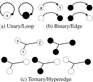
The computation ofSis performed once as a pre-processing step. The counts for any subsequent query motifMare com-puted by estimating local edge distributions usingS, without explicitly searching throughG. We now explain these cases. Computation of local distributions:The local distribution P(e)of an edge ewith no dependenciesin a motifM, is computed based on grounding of the nodes connected by the edge. For a unary relation or a directed loop such as in Fig. 4(a), we haveP(e) = #(Re)
#(Tx) when fully lifted. Here,
Tx = TypeOf(x), the entity-class of nodex, and
P(e|θx) =
1, ife∈ G,whenθx = {Tx/x},
0, otherwise.
For the binary case, fully lifted and fully grounded scenarios are computed similarly, withP(e) = #(T#(Re)
x)·#(Ty), and
P(e|θxy) =
1, ife∈ G, θxy={Tx/x,Ty/y},
0, otherwise.
(a) Unary/Loop (b) Binary/Edge
(c) Ternary/Hyperedge
Figure 4: Partial grounding in edges (Solid=ground).
Partial groundings, as shown in Fig. 4(b) (bottom), are com-puted via degree summaries:
P(e|θy) =
InG(y|e) #(Tx)·1
, whenθy = {Ty/y},
P(e|θx) =
OutG(y|e) 1·#(Ty)
, whenθx = {Tx/x}.
While the above distributions can be computed exactly, it is not as straightforward forn-ary relations, which result in hyperedges as shown in Fig. 4(c). The fully lifted and fully grounded scenarios are similar to the above cases, but han-dling partial grounding needs several assumptions:
1. Since, edge directions in ann-hyperedge are not always intuitively clear and may be domain dependent, we fol-low a partial ordering protocol described earlier.
2. Since forn > 2there can be multiple combinations of partial grounding (shown in Fig. 4(c)) and it is intractable to summarize wrt. each, we assume independence among distributions with respect to each grounded node.
When one or more source nodes are grounded θx,y = {Tx/x, Ty/y}(bottom middle in Fig. 4(c))
P(e|θx,y) =
Out
G(x|e) 1·1·#(Tz)
·
Out
G(y|e) 1·1·#(Tz)
.
However, if the sink node is grounded θZ = {Z/z}, as
show bottom right in Figure 4(c): [P(e | θz) = InG(z | e)/(#(Tx)·#(Ty)·1)].
The conditional distribution of an edge preceded by other incoming edges is accessed directly from the conditional de-pendency matrix,∆. Note that∆only captures pairwise de-pendencies and computation of arbitrary dede-pendencies can happen under certain assumptions and properties.
[Independence among incoming edges on same source]. In the motifM, if multiple incoming edgesR1, . . . ,Rj are
incident on the source nodevof the edgeRk, then the
depen-dencyP(Rk |R1, . . . ,Rj)factorizes intoQ j
i=1 P(Rk | Ri),
Algorithm 1MACH:Motif-basedApproximateCounting viaHypergraphs
1: procedureMACH(ClauseC, HypergraphG, Substitutionθ, Summary statisticsS)
2: M(VM, EM)←CONSTRUCTMOTIF(C|θ)
3: forv ∈ VMdo .Count node groundings,nv
4: ifv ∈ θthen . vis grounded inθ
5: nv←1
6: else . vis a variable inθ
7: nv←#(TypeOf(v)) .All values ofv
8: end if 9: end for 10: χ(M)←Q
v∈VMnv .Cartesian product
11: P(M)←APPROXJOINT(M,θ,G,S) .See Alg 2 12: returnχ(M)·P(M) .As given by Eqn (1)
13: end procedure
[Independence due to grounded node]. Two edges in a PGSMsharing a common node are rendered independent of each other when the shared node is already instantiated. [Independence among incoming on different source]. For ann-ary hyperedge, where multiple incoming edges are in-cident on different source nodes, we assume a similar factor-ization though the independence property no longer holds, since, constructing summaries for arbitrary dependencies is intractable. While this is astrong assumption, in many prac-tical domains, this leads to significant efficiency gains while preserving performance (see experiments).
[Incoming edge to sink is not considered for conditional dependency]. Figure 3 clearly shows, thatrb being
incom-ing on the sink node v3 of ra P(ra | rb). However, rc
considers both ra andrb as incoming, resulting inP(rc |
ra, rb). Note that, the idea generalizes to any arity.
The Algorithm: Algorithm 1 presents MACH: Motif-based Approximate Counting via Hypergraphs. As pre-processing, grounded hypergraphs are constructed and sum-marized (TYPESUM, DEGREESUM, DEPENDENCYSUM). Subsequently, for every clause, a motif is constructed and counted (using the detailed procedure APPROXJOINT pre-sented in Algorithm 2). Algorithm 2 outlines the computa-tion of the joint distribucomputa-tionP(M)for a given PGSMM. The APPROXJOINTprocedure accepts a motifM, the par-tial substitution θ of the motif, the ground hypergraph of assertions/facts G and the summaries S constructed in the
pre-processing step as the arguments and then iteratively an-alyzes each (hyper)edge inM(∀e∈ EM)[lines 3-38]. At any iteration with respect to a given (hyper)edgee, contain-ersQandVstore the nodes (ofe) which are lifted/query or instantiated/grounded, respectively, based onθ[lines 4-5].
The 3 important cases –e(1) is fully grounded, (2) fully lifted or (3) partially grounded, are handled explicitly in this procedure. [CASE 1:] Whene is fully grounded (i.e. con-tainerQ is empty), probability of edgeP(e)is set to0/1 based on whethere|θ ∈ EG [lines 7-12]. [CASE2:] When e is fully lifted (i.e. container V is empty), P(e) is com-puted as a ratio of summarized frequency of the relation type Re and the Cartesian product of the query/lifted nodes in Q, if e has no dependencies. The frequency estimates are
Algorithm 2Product of local distributions
1: procedureAPPROXJOINT(MotifM, Substitutionθ, Hyper-graphG, Summary statisticsS)
2: P(M)←1.0 .Initialize joint distribution
3: fore ∈ EMdo .For each edge in the motif
4: Q ←QUERYNODESOF(e|θ) 5: V ←GROUNDNODESOF(e|θ)
6: P(e)←1 .Initialize edge probability
7: ifQ = ∅then . e|θis fully grounded
8: ife ∈ EGthen
9: P(e)←1 . eexists in bothMandG
10: else
11: P(e)←0 . edoes not exist inG
12: end if
13: else ifV = ∅then . e|θis fully lifted 14: ifEQ=IncomingEdgesM(v) = ∅then
. v∈ Q 15: P(e)←#(Re)/Q
v∈Qnv .FromS
16: else
17: P(e)←Q Q
Q
f∈EQ P(Re|Rf) .FromS 18: end if
19: else . e|θis partially grounded
20: O, i←ORDER(V ∪ Q,θ)
21: forv ∈ Vdo .For each grounded node
22: ifv ∈ Othen .Source nodes,O
23: p←OutG(v)/Q
v∈Qnv .FromS
24: else .Sink node,i
25: p←InG(v)/Q
v∈Qnv .FromS
26: end if
27: P(e)←P(e)·p 28: end for
29: forq ∈ Qdo .For each query node
30: Eq←IncomingEdgesM(q) 31: ifEq6=∅andq∈ Othen
.Source nodes,O
32: p←Q
f∈EqP(Re|Rf) .FromS
33: end if
34: P(e)←P(e)·p 35: end for
36: end if
37: P(M)←P(M)·P(e)
38: end for 39: returnP(M)
40: end procedure
accessible from TYPESUM. In case there are dependencies (incoming edges on nodes of Q) conditionals are accessed from DEPENDENCYSUM∀v∈ Qand multiplied together2, Q
f∈EM\e P(Re|Rf),[lines 13-18]. Finally, CASE3,e be-ing partially grounded (Q 6=∅&V 6=∅), requires a more in-volved analysis[lines 20-35]. Determining the partial-order of the nodes ofeis important when computing probability of the partially-grounded (hyper)edgee.Oandimaintains the index over allsourcenodes and sink node respectively[line 20]. First we inspect all grounded nodes ofe(i.e.V). Since a grounded node nullifies any possible dependency, we need not worry about conditionals. If a grounded nodev∈ V is a source nodev∈ O, temporary distributionpw.r.t.vis given by the ratio of the out-degree ofv,OutG(v), to the
Carte-2
sian product of the type frequencies of all the lifted/query nodes. In case of a sink node,v ∈ i, the ratio is with the in-degree of the node, since the (hyper)edge eis assumed to be partially directed from the source nodes to the sink node. Note thatvhere is grounded,i.e.and actual entity is inGand the degree estimates are accessible fromS,
specif-ically DEGREESUM.P(e)is then updated with the product of the temporary distribution of allv∈ V [lines 21-28]. Fi-nally, we inspect all lifted/query nodes ofe(q ∈ Q). For any query nodeq,iff it is a source node(refer to properties & assumptions), the temporary distributionpis computed as the product of the conditionals with respect to all incoming edges onq(Q
f∈EqP(Re|Rf), wheref ∈ Eq is an incom-ing edge onqandRf is its relation type). Again,P(e)is
updated with the product of temporary distributions of all q ∈ Q[lines 29-35].P(M)is thus the product of all the factorsi.e.the edge distributions.
Theoretical properties: MACH is aimed at efficient and performance-preserving count approximations of satisfied groundings of logical clauses in Statistical Relational mod-els. Efficiency is the key aspect of the approximation strat-egy. Note, there are two distinct phases in our approach - (1) Pre-processing phase including construction of the ground hypergraph of assertions G and summaryS, and (2)
Com-puting APPROXJOINTphase. While, pre-processing has an asymptotic time complexity ofO(n2.|R|+n), wherenis the number of assertions/facts given and|R|is the number of distinct relation types in the domain, it is computed only once for a data set and is thus inconsequential.
Complexity of APPROXJOINT, however, is crucial since it is called arbitrary number of times during structure / pa-rameter learning and inference. Assuming that the summary statisticsScan be accessed efficiently, if we denote the
max-imum length of a conjunctive clause/motif ask, maximum arity of the clause/motif asAand maximum in-degree of a node in the motif asd, then the asymptotic time complexity of APPROXJOINTfor any given motifMisO(k.A.d). Most SRL systems work with reasonably small clause lengths for tractability, makingka constant. Hence, the effective com-plexity reduces toO(A.d). Cartesian product of the nodes in M (Q
v∈ VMnv) is a single operation requiring con-stant time and is inconsequential. Performance-preserving approximation requires negligible change (deterioration) in the predictive performance of an SRL model compared to its original performance with exact counts. Our evaluation re-sults corroborates our claim. APACanalysis for approxima-tion error bounds is an interesting future research direcapproxima-tion.
Experimental Evaluation
We investigate the following questions:(Q1)Is MACH ef-fective and efficient in full model learning with n-ary rela-tions compared to a robust baseline?(Q2)Is modelingn-ary relations faithfully crucial when learning relational model? and (Q3) How does MACH compare (scaling vs. perfor-mance) to a state-of-the-art database-centric MLN system?
System:We implemented MACH3using Java-based Hy-pergraphDBarchitecture (Iordanov et al. 2010), which
fa-3
Code @ https://github.com/mayukhdas/MACH
cilitates construction, operations and persistence of hyper-graphs. All database operations related to MACH are done via carefully designed Java methods using the APIs. MACH is apluggableindependent module that can be seamlessly integrated with any Java-based SRL system that uses counts. Baselines: To evaluate the effectiveness and efficiency of MACH on full structure and parameter learning of MLNs, we compared against the following baselines: (1) FACT (Das et al. 2016), which approximates counts via message-passing on normal multi-graphs, integrated with MLN-Boost and (2) basic MLN-Boost, the vanilla implementation of boosted structure and parameter learner for MLNs (Khot et al. 2011), the state-of-the-art in MLN (full) model learning without count approximations. It is reasonable to expect comparison against scalable learn-ing of MLNs (Venugopal, Sarkhel, and Gogate 2015; Sarkhel et al. 2016). However, they cannot handle partial groundings without an exponential blow-up in model / database size since they resort to creating new predicates for every grounding in a clause.
Data Sets:We used three standard SRL data sets:UW-CSE, Citeseer and WebKB, a biomedical data set Carcinogen-esis (Srinivasan et al. 1997), and an NLP/Information-Extraction(IE) data set NELL-Sports for evaluation. UWCSE is a relation-extraction/link-prediction task over an anonymized representation of staff, students and faculty of 5 different computer science departments; the target is to predict the AdvisedBy relation between faculty and students. Citeseer is a citation data set for IE, where the target is to predict which field a paper belongs to based on the title. WebKBis a consolidated data set of links among the departmental web pages of4universities, and the target is to predict if a web page is a faculty page. Carcinogen-esis is biomedical data set of the structures of chemical compounds (drugs), and the task is to predict if they are carcinogenic. NELL (Carlson et al. 2010) is a system that extracts information from online text, and converts them into a probabilistic knowledge base.NELL-Sportsis NELL data from the sports domain consisting of information about players and teams. The task is to predict whether a team plays a particular sport.
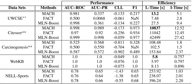
Table 1: Results: Performance vs. Efficiency (running time forLearning andInference in seconds). ** indicates n-ary predicates. Performance Efficiency
Data Sets Methods AUC–ROC AUC–PR CLL F1 L-Time [s] I-Time [s]
UWCSE∗∗
MACH 0.981 0.337 -0.133 0.217 13.2 5.1
FACT 0.500 0.0068 -0.061 NaN 7.48 2.8
MLN-Boost 0.998 0.361 -0.134 0.227 27.5 9.4
Citeseer**
MACH 0.998 0.989 -0.173 0.973 10837 12.52 FACT 0.97 0.92 -0.256 0.934 11042 12.45 MLN-Boost 0.999 0.998 -0.059 0.977 42499 27.42
Carcinogenesis**
MACH 0.525 0.568 -0.811 0.328 108.48 1.8
FACT 0.500 0.550 -0.704 NaN 102.5 1.5
MLN-Boost 0.587 0.572 -0.902 0.489 153.84 2.37
WebKB
MACH 1.0 1.0 -0.049 1.0 5.8 0.757
FACT 1.0 1.0 -0.076 1.0 5.97 0.797
MLN-Boost 1.0 1.0 -0.075 1.0 8.13 0.896
NELL-Sports
MACH 0.78 0.65 -1.43 0.65 253.92 1.03
FACT 0.76 0.64 -1.38 0.65 238.07 2.01
MLN-Boost 0.78 0.66 -0.55 0.68 396.24 2.20
Table 2: Performance vs. Efficiency (running time for Inference in seconds) compared againstTuffy.
Data Sets System AUC-ROC I-Time [s]
UW-CSE MACH 0.892 20.06
Tuffy 0.877 37.11
Carcinogenesis MACH 0.524 199.8
Tuffy 0.560 944.98
R(v1, . . . ,vn),n > 2 as {Rij(vi,vj)}, (i < j), that is
i∈[1, n),j∈(i, n]. We modify the assertions based on the new relations as well. Observe that, though the efficiency gain is equivalent to (and at times better than) MACH, there is a significant deterioration in performance, especially on the relatively smaller data sets. In the case of a large data set such asCiteseer, the performances are relatively similar since the number of spurious assertions introduced by the decomposition ofn-ary relations are negligible compared to the sheer size of the original data set. In contrast, this size difference is not prevalent in smaller data sets, which results in worse predictive performance compared to MLN-Boost and MACH. Thus, it is critical thatn-ary relations are repre-sented faithfully, which answers(Q2)affirmatively. (Q3: HypergraphDB versus DB) In order to evaluate against a database-centric MLN system, we compared MACH with Tuffy(Niu et al. 2011). While Tuffy is a ro-bust MLN engine integrated with PostgreSQL RDBMS, an unbiased comparison with our system is challenging. This is because, although Tuffyhas no restrictions on the type (discriminative vs. generative) of MLNs (unlike MLN-Boost which can only represent discriminative MLNs via Horn clauses), it does not support structure learning (which MLN-Boost can perform, simultaneously with parameter learn-ing). In order to keep the comparison fair, we learn MLNs via MLN-Boost, convert it intoTuffyformat, and then com-pare the inference performance and efficiency with MACH. MACH was integrated with the inference engine of MLN-Boost directly. Table 2 summarizes the results. Observe how
MACH shows significant gain in efficiency, while being at par with Tuffy’s performance. Since Tuffyreports time in-clusive of setup and post-processing, we did the same for MACH. Note that inference time of MACH for UW-CSE is 20.06 sec., which is almost twice as fast as Tuffy, in-cludes the setup and hypergraph construction and summa-rization time of 13.26sec. On Carcinogenesiswe observe that MACH is approximately 5 times as fast (w/ 192.2s. setup time). The performances are almost equivalent, though the inference algorithms are different. This allows us to an-swer(Q3)affirmatively. Finally, note thatTuffyinfers on all possible instances of the target. For fair comparison we de-activate sub-sampling of negative examples in MLN-Boost.
Conclusion
We present a method for approximating counts of logical rules in SRL models via transforming both the clauses and the full set of groundings into a hypergraph. We showed how counting the number of subgraphs in these hypergraphs cor-respond to counting the number of groundings in the SRL model. We presented the use of summary statistics to ap-proximate this count. There are several possible directions to extend our work - first is more rigorous evalation on large data sets across other models. Second is that is while in our work we consider only conjunctions, extending the idea to count over arbitrary clauses. Finally, combining our method with methods such as FROG (Shavlik and Natarajan 2009) that eliminates trivial groundings of clauses can potentially allow our algorithm to be employed in real large data sets.
Acknowledgements
government. Parts of this work grew out of discussions of KK within the DFG Research Training Group GRK 1994.
References
Berge, C., and Minieka, E. 1973. Graphs and hypergraphs. North-Holland Publishing Company Amsterdam.
Bhaskara, A.; Charikar, M.; Chlamtac, E.; Feige, U.; and Vi-jayaraghavan, A. 2010. Detecting high log-densities: An O(N14)approximation for densest K-subgraph. InSOTC. Carlson, A.; Betteridge, J.; Kisiel, B.; Settles, B.; Hr-uschka Jr, E.; and Mitchell, T. 2010. Toward an architecture for never-ending language learning. InAAAI.
Corby, O.; Dieng, R.; and H´ebert, C. 2000. A conceptual graph model for W3C resource description framework. In ICCS.
Das, M.; Wu, Y.; Khot, T.; Kersting, K.; and Natarajan, S. 2016. Scaling Lifted Probabilistic Inference and Learning Via Graph Databases. InSDM.
Demeyer, S.; Michoel, T.; Fostier, J.; Audenaert, P.; Pick-avet, M.; and Demeester, P. 2013. The index-based subgraph matching algorithm (ISMA): Fast subgraph enumeration in large networks using optimized search trees. PLOS One.
Domingos, P., and Lowd, D. 2009.Markov Logic: An Inter-face Layer for AI. M & C.
Dudek, A.; Frieze, A.; Ruci´nski, A.; and ˇSileikis, M. 2013. Approximate counting of regular hypergraphs. Information Processing Letters.
Dudek, A.; Karpinski, M.; Ruci´nski, A.; and Szyma´nska, E. 2014. Approximate counting of matchings in (3,3)-hypergraphs. InAlgorithm Theory – SWAT 2014.
Feng, F.; He, X.; Liu, Y.; Nie, L.; and Chua, T.-S. 2018. Learning on partial-order hypergraphs. InWWW.
F¨urer, M., and Kasiviswanathan, S. P. 2014. Approximately counting embeddings into random graphs. Combinatorics, Probability and Computing.
Getoor, L., and Taskar, B. 2007. Introduction to Statistical Relational Learning. MIT Press.
Iordanov, B.; Vandev, K.; Costa, C.; Marinov, M.; Saraiva de Queiroz, M.; Holsman, I.; Picard, A.; and Bogdahn, I. 2010. HyperGraphDB 1.3.
Kersting, K.; Ahmadi, B.; and Natarajan, S. 2009. Counting Belief Propagation. InUAI.
Khot, T.; Natarajan, S.; Kersting, K.; and Shavlik, J. 2011. Learning Markov logic networks via functional gradient boosting. InICDM.
Neumann, T., and Moerkotte, G. 2011. Characteristic sets: Accurate cardinality estimation for rdf queries with multiple joins. InICDE.
Niu, F.; R´e, C.; Doan, A.; and Shavlik, J. W. 2011. Tuffy: Scaling up Statistical Inference in Markov Logic Networks using an RDBMS.PVLDB.
Poole, D. 2003. First-Order Probabilistic Inference. In IJ-CAI.
Raedt, L. D.; Kersting, K.; Natarajan, S.; and Poole, D. 2016. Statistical relational artificial intelligence: Logic, probability, and computation.Synthesis Lect. on AI & ML. Ravkic, I.; Znidarsic, M.; Ramon, J.; and Davis, J. 2018. Graph sampling with applications to estimating the number of pattern embeddings and the parameters of a statistical re-lational model.Data Min. Knowl. Discov.32.
Sarkhel, S.; Venugopal, D.; Pham, T.; Singla, P.; and Gogate, V. 2016. Scalable training of Markov logic networks using approximate counting. InAAAI.
Schiefer, B.; Strain, L. G.; and Yan, W. P. 1998. Method for estimating cardinalities for query processing in a relational database management system. US Patent 5,761,653. Seputis, E. A. 2000. Database system with methods for per-forming cost-based estimates using spline histograms. US Patent 6,012,054.
Shavlik, J., and Natarajan, S. 2009. Speeding up inference in Markov logic networks by preprocessing to reduce the size of the resulting grounded network. InIJCAI.
Slota, G. M., and Madduri, K. 2013. Fast approximate sub-graph counting and enumeration. InIntl. Conf. on Parallel Processing.
Srinivasan, A.; King, R. D.; Muggleton, S. H.; and Stern-berg, M. 1997. Carcinogenesis predictions using ILP. In-ductive Logic Programming.
Stocker, M.; Seaborne, A.; Bernstein, A.; Kiefer, C.; and Reynolds, D. 2008. Sparql basic graph pattern optimiza-tion using selectivity estimaoptimiza-tion. InWWW.
Vadhan, S. P. 2001. The complexity of counting in sparse, regular, and planar graphs. SICOMP.
Valiant, L. G. 1979. The complexity of enumeration and reliability problems. SICOMP.