NetSDM: Semantic Data Mining with Network Analysis

(1)

NetSDM: Semantic Data Mining with Network Analysis

Jan Kralj jan.kralj@ijs.si

Joˇzef Stefan Institute, Department of Knowledge Technologies, Jamova 39, 1000 Ljubljana, Slovenia

Marko Robnik-ˇSikonja marko.robnik@fri.uni-lj.si

University of Ljubljana, Faculty of Computer and Information Science, Veˇcna pot 113, 1000 Ljubljana, Slovenia

Nada Lavraˇc nada.lavrac@ijs.si

Joˇzef Stefan Institute, Department of Knowledge Technologies, Jamova 39, 1000 Ljubljana, Slovenia

Editor:Bert Huang

Abstract

Semantic data mining (SDM) is a form of relational data mining that uses annotated data together with complex semantic background knowledge to learn rules that can be easily interpreted. The drawback of SDM is a high computational complexity of existing SDM algorithms, resulting in long run times even when applied to relatively small data sets. This paper proposes an effective SDM approach, named NetSDM, which first transforms the available semantic background knowledge into a network format, followed by network analysis based node ranking and pruning to significantly reduce the size of the original background knowledge. The experimental evaluation of the NetSDM methodology on acute lymphoblastic leukemia and breast cancer data demonstrates that NetSDM achieves radical time efficiency improvements and that learned rules are comparable or better than the rules obtained by the original SDM algorithms.

Keywords: data mining, semantic data mining, ontologies, subgroup discovery, network analysis

1. Introduction

In data mining applications, relevant information can be scattered across disparate resources in heterogeneous data formats. Extraction of knowledge from large heterogeneous data is technically challenging and time consuming, and presents a significant obstacle to wider adoption of data mining in real-life applications. While most of the data mining algorithms

(Witten and Frank, 2005) work only with tabular data, relational data mining (RDM)

(Dˇzeroski and Lavraˇc, 2001) andrelational learning (De Raedt, 2008) algorithms can use

additional relational information about the analyzed data to build richer and more accurate predictive models. One such form of additional information is domain knowledge (relational background knowledge) about instances of a data set. As shown by Page et al. (2012) and Peissig et al. (2014), relational data mining can significantly outperform classical machine learning approaches.

Previous work on RDM has shown that the use of background knowledge is vital for

data analysis in many domains. However, the issue with using more complex data (i.e.,

c

(2)

data along with relations and background knowledge) is that it can no longer be easily represented in a tabular format (also referred to as a design matrix (Rendle, 2013)). Better data representations are needed when instances under examination are interconnected to a various (non-fixed) number of instances. Representing each connection from an instance as a separate column would result in a different number of columns for each row. Alternatively, if we encoded connections of an instance with a single column, columns would have to contain composite data structures such as lists. In RDM, this problem is addressed by representing

data sets withmulti-relational databases and by applying specialized relational data mining

algorithms for data analysis (Dˇzeroski and Lavraˇc, 2001). Examples of such instances are

genes that are connected through mutual activation, or research papers connected through citations.

An alternative way to describe a data set containing inter-connected instances is to

represent it as a network (Burt and Minor, 1983), a data structure containing nodes,

in-formation about the nodes, and connections between the nodes. In mathematical terms,

such a structure is described as a graph, where the nodes are referred to as vertices, and

the connections as edges. The field of network analysis deals with several types of

net-works. In social networks, nodes represent people and connections represent their social links. Biological networks include gene regulatory networks, protein interaction networks, drug interaction networks, etc. In information networks, directed connections encode

in-formation flow between the network nodes. While most researchers deal with homogeneous

information networks, where all nodes and edges are of the same node/edge type, Sun and

Han (2012) addressed the problem of heterogeneous information network analysis, where

nodes and edges belong to different node or edge types. For example, we may have a network containing both the genes and the proteins they encode, which necessitates the use of two

node types to represent the data. Sun and Han (2012) introduced the concept ofauthority

ranking for heterogeneous information networks, where the impact of a node is transferred along the edges to simultaneously rank nodes of different types, while class labels can also be propagated through the network (Vanunu et al., 2010).

Network analysis can be considered as a form of relational learning, where instances are linked by relations and connected in a complex graph. Special form of relational data are ontologies (Guarino et al., 2009). The challenge of incorporating domain ontologies in

the data mining process has been addressed in the work on semantic data mining (SDM)

(Lavraˇc and Vavpetiˇc, 2015). Semantic data mining can discover complex rules describing

subgroups of data instances that are connected to terms (annotations) of an ontology, where the ontology is referred to as background knowledge used in the learning process. An example SDM problem is to find subgroups of enriched genes in a biological experiment, where background knowledge is the Gene Ontology (Ashburner et al., 2000).

Given that SDM algorithms are relatively slow, the size of the background knowledge used by SDM approaches is usually several orders of magnitude lower than the problems typically handled by network analysis approaches. Take for example SDM algorithm Hedwig

(Vavpetiˇc et al., 2013), which is one of the semantic data mining algorithm used in this work.

(3)

take a SDM application where Hedwig was applied to a data set of 337 examples and

a background knowledge of 21,062 interconnected ontology terms (Vavpetiˇc et al., 2013),

which is small compared to typical network analysis applications that deal with much larger data sets, possibly composed of e.g., hundred millions network nodes.

Despite large differences in the current sizes of data sets analyzed by SDM and network analysis approaches, the two research fields are aligned in terms of the research question

of interest, which can be posed as follows: Which part of the network structure is the most

important for the analyst’s current query? The challenge addressed in this work is the reduction of the search space of SDM algorithms, which can be achieved by using network analysis approaches. To this end, we have developed an approach that is capable of utiliz-ing network analysis algorithms Personalized PageRank (Page et al., 1999) and node2vec (Grover and Leskovec, 2016) to improve the efficiency of SDM. We show that the proposed approach, named NetSDM, can efficiently generate high quality rules by investigating only a fraction of the entire search space imposed by the background knowledge considered.

The rest of the paper is structured as follows. Section 2 presents the related work, as well as the technologies used; we first introduce the semantic data mining algorithms used, Hedwig and Aleph (Srinivasan, 1999), and then present the two network analysis algorithms, Personalized PageRank and node2vec. Section 3 presents the proposed NetSDM approach that exploits network analysis to reduce the size of the background knowledge used by SDM algorithms. Section 4 presents the experimental setup, and Section 5 presents the experimental results. Section 6 concludes the paper and presents plans for further work.

2. Related work and background technologies

This section presents the related work in the fields of semantic data mining and network analysis. It starts with the related work in the field of semantic data mining in Section 2.1, which presents also the two algorithms used in our experiments: Hedwig and Aleph. It continues with the related work in the field of network analysis in Section 2.2, and includes the two algorithms used in our experiments: Personalized PageRank and node2vec.

2.1. Semantic data mining

To find patterns in data annotated with ontologies, we rely on semantic data mining (SDM)

(Dou et al., 2015; Lavraˇc and Vavpetiˇc, 2015). In SDM, the input is composed of a set of

class labeled instances and the background knowledge encoded in the form of ontologies, and the goal is to find descriptions of target class instances as a set of rules of the form

TargetClass ← Explanation, where the explanation is a logical conjunction of terms from the ontology. Semantic data mining has its roots in symbolic rule learning, subgroup discovery and enrichment analysis research, briefly explained below.

2.1.1. Rule learning and subgroup discovery

One of the established techniques for data mining (Piatetsky-Shapiro, 1991) is symbolic

rule learning (F¨urnkranz et al., 2012). While rule learning was initially focused on learning

(4)

aims at finding interesting descriptive patterns in the unsupervised as well as in supervised learning settings (Liu et al., 1998).

Building on classification and association rule learning, subgroup discovery techniques

aim at finding interesting patterns as sets of rules that best describe the target class (Kl¨osgen,

1996; Wrobel, 1997). Typical output of subgroup discovery algorithms are rules where the

rule condition (Explanation) is a conjunction of features (attribute values) that

charac-terize the target class instances covered by the rule, and each rule describes a particular interesting subgroup of target class instances.

2.1.2. Using ontologies in enrichment analysis

Enrichment analysis (EA) techniques are statistical methods used to identify putative ex-planations for a set of entities based on over- or under-representation of their attribute

values, which can be referred to as differential expression. In life sciences, EA is widely

used with the Gene Ontology (GO) (Ashburner et al., 2000) to profile the biological role of genes, such as differentially expressed cancer genes in microarray experiments (Tipney and Hunter, 2010).

While standard EA provides explanations in terms of concepts from a single ontology, researchers are increasingly combining several ontologies and data sets to uncover novel associations. The ability to detect patterns in data sets that do not use only the GO can yield valuable insights into diseases and their treatment. For instance, it was shown that Werner’s syndrome, Cockayne syndrome, Burkitt’s lymphoma, and Rothmund-Thomson syndrome are all associated with aging related genes (Puzianowska-Kuznicka and Kuznicki, 2005; Cox and Faragher, 2007). On the clinical side, EA can be used to learn adverse events from Electronic Health Record (EHR) data such as increased comorbidities in rheumatoid arthritis patients (LePendu et al., 2013), or to identify phenotypic signatures of neuropsychi-atric disorders (Lyalina et al., 2013). An ontology-based EA approach was used to identify genes linked to aging in worms (Callahan et al., 2015), aberrant pathways—the network drivers in HIV infection identifying HIV inhibitors strongly associated with mood disorders (Hoehndorf et al., 2012), or to learn a combination of molecular functions and chromosome positions from lymphoma gene expression (Jiline et al., 2011).

2.1.3. Using ontologies in rule learning

An abundance of taxonomies and ontologies that are readily available can provide higher-level descriptors and explanations of discovered subgroups. In the domain of systems biology the Gene Ontology (Ashburner et al., 2000), KEGG orthology (Ogata et al., 1999) and Entrez gene–gene interaction data (Maglott et al., 2005) are examples of structured domain knowledge. In rule learning, the terms in the nodes of these ontologies can take the role of additional high-level descriptors (generalizations of data instances) used in the induced rules, while the hierarchical relations among the terms can be used to guide the search for conjuncts of the induced rules.

(5)

combinations of Gene Ontology (GO) terms, KEGG orthology terms, and terms describing gene–gene interactions obtained from the Entrez database.

The challenge of incorporating domain ontologies in data mining was addressed in SDM

research by several other authors. ˇZ´akov´a et al. (2006) used an engineering ontology of

Computer-Aided Design (CAD) elements and structures as a background knowledge to extract frequent product design patterns in CAD repositories and to discover predictive rules from CAD data. Using ontologies, the algorithm Fr–ONT for mining frequent concepts was introduced by Lawrynowicz and Potoniec (2011).

Vavpetiˇc and Lavraˇc (2013) developed a SDM toolkit that includes two semantic data

mining systems: SDM-SEGS and SDM-Aleph. SDM-SEGS is an extension of the ear-lier domain-specific algorithm SEGS (Trajkovski et al., 2008a), which supports semantic subgroup discovery in gene expression data. SDM-SEGS extends and generalizes this ap-proach by allowing the user to input a set of ontologies in the OWL ontology specification language and an empirical data set annotated with domain ontology terms. SDM-SEGS employs a predefined selection of ontologies to constrain and guide a top-down search of the hierarchically structured hypothesis space. SDM-Aleph is an extension of the Inductive Logic Programming system Aleph (Srinivasan, 1999), which does not have the limitations of SDM-SEGS imposed by domain-specific properties of algorithm SEGS, and can accept any number of ontologies as domain background knowledge, including different relations.

In summary, semantic subgroup discovery algorithms SDM-SEGS and SDM-Aleph are either specialized for a specific domain (Trajkovski et al., 2008b) or adapted from systems

that do not take into account the hierarchical structure of background knowledge (Vavpetiˇc

and Lavraˇc, 2013), respectively. Therefore in this work, we rather use the Hedwig algorithm

(Vavpetiˇc et al., 2013) and the original Aleph algorithm (Srinivasan, 1999), which can both

accept any number of input ontologies, where Aleph can also use different types of relations.

2.1.4. Hedwig

Figure 1: An example output of the Hed-wig semantic subgroup discovery

algorithm, where Explanations

represent subgroups of genes, differentially expressed in pa-tients with breast cancer. To illustrate the rules induced by the Hedwig

subgroup discovery algorithm (Vavpetiˇc et al.,

2013), take as an example a task of analyzing differential expression of genes in breast can-cer patients, originally addressed by Sotiriou

et al. (2006). In this task, the TargetClass

of the generated rules is the class of genes that are differentially expressed in breast cancer pa-tients as compared to the general population. The Hedwig algorithm generated ten rules (subgroup descriptions), each describing a sub-group of differentially expressed genes. In the

rules, the TargetClass is the set of

differen-tially expressed genes and theExplanationis

a conjunction of Gene Ontology terms and cov-ers the set of genes annotated by the terms in

(6)

Take the first ranked rule, where theExplanationis a conjunction of biological concepts

chromosome ∧ cell cycle, which covers all the genes that are covered by both ontology

terms. Take as another example the fourth best ranked rule, which explains that the

regulation of the mitotic cell cycle and cytoskeletal formation explain the breast cancer based on gene expression.

The semantic subgroup discovery task addressed by Hedwig takes three types of inputs: the training examples, the domain knowledge, and a mapping between the two.

• Data set, composed of training examples expressed as RDF (Resource Description

Framework) triples in the form subject-predicate-object, e.g., geneX–suppresses–geneY.

Data set S is split into a set of positive examples S+, i.e. ‘interesting’ target class

instances (for example, genes enriched in a particular biological experiment), and a

set of negative examplesS− of non-target class instances (e.g., non-enriched genes).

• Domain knowledge, composed of domain ontologies in RDF form.

• Object-to-ontology mapping, which associates each RDF triple with an appropriate

ontological concept. We refer to these object-to-ontology mappings as annotations,

meaning that object x is annotated by ontology term o if the pair (x, o) appears in

the mapping.

For given inputs, the output of Hedwig is a set of descriptive patterns in the form of rules, where rule conditions are conjunctions of domain ontology terms that explain a group of target class instances. Ideally, Hedwig discovers explanations that best describe and cover as many target class instances and as few non-target instances as possible.

The Hedwig algorithm uses beam search, where the beam contains the best N rules. It starts with the default rule that covers all the training examples. In every search iteration, each rule from the beam is specialized via one of the four operations: (i) replace the predicate of a rule with a predicate that is a sub-class of the previous one, (ii) negate a predicate of a rule, (iii) append a new unary predicate to the rule, or (iv) append a new binary predicate, introducing a new existentially quantified variable, where the new variable has to be ‘consumed’ by a literal that has to be added as a conjunction to this clause in the next step of rule refinement.

Hedwig learns rules through a sequence of specialization steps. Each step either main-tains or reduces the current number of covered examples. A rule will not be specialized once its coverage is zero or falls below some predetermined threshold. When adding a new conjunct, the algorithm checks if the specialized rule improves the probability of rule

consequent—to this end the redundancy coefficient is used (Hämäläinen, 2010); if not, the

specialized rule is not added to the list of specializations. After the specialization step is

applied to each rule in the beam, a new set of best scoring N rules is selected. If no

im-provement is made to the rule collection, the search terminates. In principle, the procedure supports any rule scoring function. Numerous rule scoring functions for discrete targets are

available: χ2, Precision, WRAcc (Lavraˇc et al., 2004), Leverage, and Lift. Note that Lift is

the default measure in Hedwig (see Section 2.1.6) that was used in our experiments.

In addition to an illustrative financial use case (Vavpetiˇc et al., 2013), Hedwig was

shown to perform well in breast cancer data analysis (Vavpetiˇc et al., 2014), as well as in a

(7)

et al., 2016), where it was a part of three-step methodology, together with mixture models and banded matrices using several ontologies obtained from various sources: hierarchical structure of multiresolution data, chromosomal location of fragile sites, virus integration sites, cancer genes, and amplification hotspots.

2.1.5. Aleph

Aleph (A Learning Engine for Proposing Hypotheses) (Srinivasan, 1999) is a general pur-pose system for Inductive Logic Programming (ILP) that was conceived as a workbench for implementing and testing concepts and procedures from a variety of different ILP and rela-tional learning systems and papers. The system can construct rules, trees, constraints and features; invent abnormality predicates; perform classification, regression, clustering, and association rule learning; allows for choosing between different search strategies (general-to-specific or specific-to-general, i.e. top-down or bottom-up, bidirectional, etc.), search algorithms (hill-climbing, exhaustive search, stochastic search, etc.) and evaluation func-tions. It allows users to specify their own search procedure, proof strategy, and visualization of hypotheses.

Similarly to Hedwig, Aleph accepts as input a set of positively and negatively labeled training examples and a file describing the background knowledge, including a mapping between the examples and the background knowledge. The training examples are expressed as Prolog facts, and the background knowledge is in the form of Prolog facts and clauses. In contrast to Hedwig that was used in our experiments for semantic subgroup discovery, we used Aleph in its default operation mode to learn a classifier (a Theory) composed of as a set of classification rules, which also explain the target class examples.

Aleph constructs rules in several steps. It first selects a positive example and builds the most specific rule explaining the example following the steps described by Muggleton (1995). Next, the algorithm searches for a more general rule, performed with a branch-and-bound search strategy, searching first through generalizations of the rule containing the fewest terms. Finally, the rule with the best score is added to the current theory, and all the examples covered by this rule are removed (this step is sometimes called the ”cover removal” step). This procedure is repeated until all the positive examples are covered.

Aleph was incorporated into the SDM-toolkit (Vavpetiˇc and Lavraˇc, 2013), which allows

Aleph (named SDM-Aleph) to use the same input data as Hedwig. However, a drawback of using SDM-Aleph is that it can reason only over one type of background knowledge relations, while the original Aleph algorithm can reason over any type of relations. In the case of Gene Ontology, which was used as the background knowledge in our experiments,

this generality allows Aleph to encode both theis a and is part of relations, which are the

most frequent relations in ontologies, as well as the relationships composed of these two relations.

2.1.6. Rule quality measures

We use several measures to evaluate the quality of rules discovered by Hedwig and Aleph.

Take for example ruleR with a condition that is true for 80 positive instances (True

Pos-itives, T P) and 20 negative instances (False Positives,F P) from the setS of 100 positive

(8)

100 is the total number of instances covered by the rule. Support of the rule is calculated

as follows: Support(R) = T P_|+_S_|F P = Coverage(R)_|_S_| = 0.5. Precision(R) = 0.8 is calculated as

T P

T P+F P, and Accuracy(R) = 0.8 is calculated as

T P+T N

|S| , whereT N denotes the number of

True Negatives.

In our experiments we use the Lift metric to evaluate the performance of SDM algorithms

Hedwig and Aleph. Lift(R) is defined as the ratio between the precision of a rule and the

proportion of positive examples in the data set (i.e. the precision of the empty default

rule that classifies all examples as positive). In our example Lift(R) = 0₀._.8₅ = 1.6, which is

calculated using the following formula:

Lift(R) = Precision(R)

P R (1)

whereP R= |P ositives_|_S_| | is the ratio of positive instances in the data set. The range of values

Lift can take is from 0 to ∞ and larger values indicate better rules.

2.2. Network analysis

Network analysis uses concepts from graph theory to investigate characteristics of networked structures in terms of nodes (such as individual actors, people, or any other objects in the network) and edges or links that connect them (relationships, interactions or ties between the objects). This section focuses on the algorithms which we used or adapted to rank nodes in information networks.

2.2.1. Node ranking: Using Personalized PageRank algorithm

The objective of node ranking in information networks is to assess the relevance of a given node either globally (with regard to the whole graph) or locally (relative to some other node

or group of nodes in the graph). A network node ranking algorithm assigns a score (or a

rank) to each node in the network, with the goal of ranking the nodes in terms of their

relevance.

A well known node ranking method is PageRank (Page et al., 1999), which was used in the Google search engine. Other methods for node ranking include Weighted PageRank method (Xing and Ghorbani, 2004), SimRank (Jeh and Widom, 2002), diffusion kernels (Kondor and Lafferty, 2002), hubs and authorities (Kleinberg, 1999), and spreading acti-vation (Crestani, 1997). More recent network node ranking methods include PL-ranking (Zhang et al., 2016) and NCDawareRank (Nikolakopoulos and Garofalakis, 2013). Another way to rank nodes in a network is to use network centrality measures, such as Freeman’s network centrality (Freeman, 1979), betweenness centrality (Freeman, 1977), closeness cen-trality (Bavelas, 1950), and Katz cencen-trality (Katz, 1953).

(9)

starting nodes, in our case, those representing the positive examples. In the context of data set annotation with ontologies, this allows us to estimate the importance of background knowledge terms in relation to the positive examples in the data set.

Personalized PageRank uses a random walk approach to calculate the significance of

nodes in an information network. Given a set of ‘starting’ nodesA, the Personalized

PageR-ank calculated for A (denoted P-PRA) is defined as the stationary distribution of random

walker positions, where the walk starts in a randomly chosen member ofAand then at each

step either selects one of the outgoing connections or teleports back to a randomly selected

member of A. Probability p of continuing the walk is a parameter of the Personalized

PageRank algorithm and is usually set to 0.85. In our context, the P-PR algorithm is used

to calculate the importance of network nodeswith respect to a given set of starting nodes.

Remark 1 P-PRA is a vector, and each value of the vector corresponds to some network

nodeu. Ifuis thei-th node of the network, notation P-PRA(u)is used (rather than P-PRAi)

to denote the i-th value of P-PRA.

2.2.2. Network embedding: Using node2vec algorithm

Network embedding is a mechanism for converting networks into a tabular/matrix repre-sentation format, where each network node is represented as a vector of some predefined

fixed length k, and a set of nodes is represented as a table with k columns. The goal of

such a conversion is to preserve structural properties of a network, which is achieved by preserving node similarity in both representations, i.e. node similarity is converted into vector similarity.

Network nodes vectorization can be effectively performed by the node2vec algorithm (Grover and Leskovec, 2016), which uses a random walk approach to calculate features that express the similarities between node pairs. The node2vec algorithm takes as input a

network ofnnodes, represented as a graph G= (V, E), where V is the set of nodes and E

is the set of edges in the network. For a user-defined number of columns k, the algorithm

returns a matrixf∗ ∈R|V|×k, defined as follows:

f∗ = node2vec(G) = argmax

f∈R|V|×k X

u∈V



−log(Zu) +

X

n∈N(u)

f(n)·f(u)



 (2)

whereN(u) denotes the network neighborhood of nodeu (to be defined below).

Remark 2 Each matrixf is a collection of k-dimensional feature vectors, with thei-th row of the matrix corresponding to the feature vector of thei-th node in the network. We write

f(u) to denote the row of matrix f corresponding to node u.

The goal of the node2vec algorithm is to construct feature vectors f(u) in such a way

that feature vectors of nodes that share a certain neighborhood will be similar. The inner

sum of the value, maximized in Equation 2, calculates the similarities between node u

(10)

norm. Next, value Zu calculates the similarities between node u and all the nodes in the

network as follows:

Zu =

X

v∈V

ef(u)·f(v)

Note that value of −log(Zu) decreases when the norms of feature vectors f(v) increase,

thereby penalizing collections of feature vectors with large norms.

Equation 2 has a probabilistic interpretation that models a process of randomly selecting

nodes from the network (Grover and Leskovec, 2016). In this process, probability P(n|u)

of node n following nodeu in the selection process is proportional to ef(n)·f(u). Assuming

that selecting a node is independent from selecting any other node, we can calculate the

probability of selecting all nodes from a given set N as P(N|u) = Q

n∈NP(n|u), and

Equation 2 can then be rewritten as follows:

f∗ = node2vec(G) = argmax

f∈_R|V|×k

X

u∈V

log (P(N(u)|f(u))) (3)

Finally, let us explain neighborhoodN(u) in Equations 2 and 3, calculated by simulating

a random walker traversing the network starting at node u. Unlike the PageRank random

walker, the transition probabilities for traversing from noden1 to noden2 depend on node

n0 that the walker visited before noden1, making the process of traversing the network a

second order random walk. The non-normalized transition probabilities are set using two

parameters,p and q, and are equal to:

P(n2|moved from noden0 ton1 in previous step) =

  

  1

p ifn2 =n0

1 ifn2 can be reached fromn1

1

q otherwise

The parameters of the expression are referred to as the return parameterp and thein-out

parameter q. A low value of the return parameter p means that the random walker is

more likely to backtrack its steps and the random walk will be closer to a breadth first

search. On the other hand, a low value of parameterq encourages the walker to move away

from the starting node and the random walk resembles a depth first search of the network.

To calculate the maximizing matrix f∗, a set of random walks of limited size is simulated

starting from each node in the network to generate several samples of sets N(u).

The function maximizing Equation 2 is calculated using the stochastic gradient descent.

The matrix of feature vectors node2vec(G) in Equation 2 is estimated at each generated

sampling of neighborhoods N(u) for all nodes in the network to discover matrix f∗ that

maximizes the expression for the simulated neighborhood set.

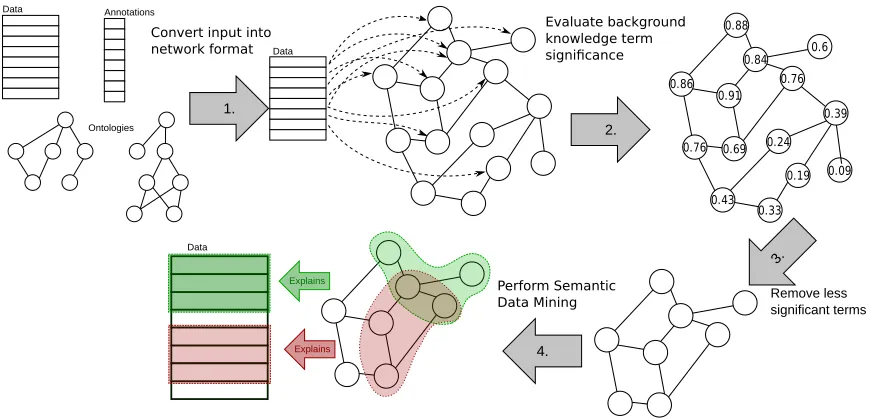
3. NetSDM methodology: Combining SDM with network analysis

(11)

Evaluate background knowledge term signiﬁcance

Data

4.

2. 1.

3.

Remove less significant terms

Data Annotations

Ontologies

Convert input into network format

Perform Semantic Data Mining

0.88

0.86 0.91

0.69 0.76

0.43 0.33

0.19 0.24

0.39

0.09 0.76

0.6 0.84

Explains

Figure 2: Illustrative outline of the proposed NetSDM methodology.

NetSDM methodology that combines semantic data mining with network analysis to reduce the search space of SDM algorithms. This section starts with an overview of the proposed methodology in Section 3.1, illustrated by an example in Section 3.2. Section 3.3 provides a detailed step-by-step description of the NetSDM methodology.

3.1. Methodology outline

SDM algorithms use heuristic search when mining for patterns in the data to limit the search to only the most promising parts of the search space. Constraining the search is necessary, as traversing the entire search space—consisting of conjuncts of logical expres-sions containing ontological expresexpres-sions—is computationally unfeasible. However, heuristic search can produce poor results in some cases. For example, when searching for patterns with Hedwig using beam search, the beam may be too narrow, and consequently a branch that would lead to a high quality solution could be discarded early on; in large search spaces even wide beams can be quickly filled with terms that do not lead to good final solutions. Similarly, the search algorithm in Aleph can miss important patterns if all their sub-patterns exhibit low quality. In this paper we propose a new methodology, which aims to solve this problem. The proposed NetSDM methodology, which is illustrated in Figure 2, consists of the following four steps:

1. Convert a background knowledge ontology into a network format.

2. Estimate the importance of background knowledge terms using a scoring function.

3. Shrink the background knowledge, keeping only a proportion c of the top ranking

terms.

(12)

Input: SDM algorithm, network conversion method, scoring function, term

removal method, background knowledge ontology O, set of examplesS

annotated with terms from O

Output: set of rules discovered by SDM algorithm Parameters: shrinkage coefficient c∈[0,1]

1 Convert ontologyO into network format G_e (see Section 3.3.1)

2 Calculate significance scoresscore(t), for all terms t∈ T(O) (see Section 3.3.2)

3 for term t∈ T(O) do

4 if RelativeRank(t)> c then

5 mark term tfor removal.

6 end

7 end

8 formG_e0 by removing marked terms fromG_e (see Section 3.3.3)

9 convert G_e0 toO0

10 Run SDM algorithm onS using reduced background knowledgeO0

11 return Rules discovered by SDM algorithm

Algorithm 1: The NetSDM algorithm, implementing the proposed approach to semantic data mining with network node ranking and ontology shrinking.

The NetSDM methodology improves the efficiency of SDM algorithms by using a shrink-ing step in which we filter out background knowledge terms that are not likely to appear in significant rules. The methodology is implemented in Algorithm 1. A scoring function used in ontology shrinkage should (i) be able to evaluate the significance of terms based on the data, and (ii) be efficiently computed.

The input for the scoring function is the data used in SDM algorithms, consisting of:

• Set of instancesS consisting of target (S+) and non-target (S−) instances,

• OntologyOrepresented as a set of RDF triples (subject, predicate, object) (to simplify

the notation, for each term t appearing as either a subject or object in a triple, we

will write t∈O to denote thatt is a term of the ontologyO),

• Set of annotationsAconnecting instances inS=S+∪S−with terms inO(annotations

are presented as triples (s,annotated-with, t), where s ∈ S and t ∈ O denoting that

data instancesis annotated by an ontology term t.

The output of the scoring function is a vector which, for each term in the background

knowledge, contains a score estimating its significance. In other words, using T(O) to

denote the set of all terms appearing (either as subjects or objects) in ontology O, the

scoring function is defined as:

scoreS,O,A :T(O)→[0,∞)

After defining a suitable scoring functionscore (in the subsequent subsections, we examine

(13)

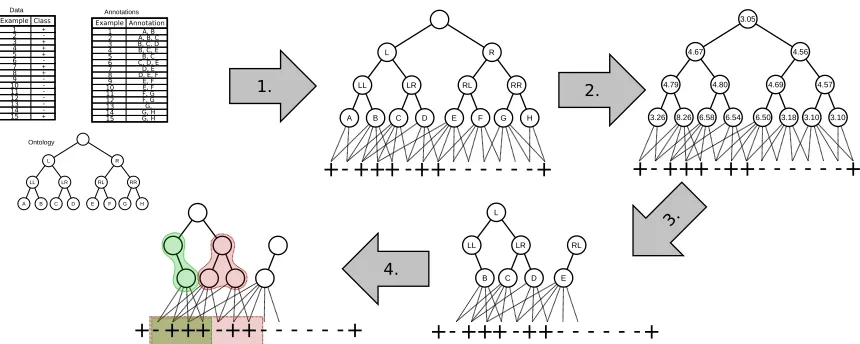
3.26 8.26 6.58 6.54 6.50 3.18 3.10 3.10 4.79 4.80 4.69 4.57

4.56 4.67

3.05

A B C D E F G H

LL LR RL RR

L R

L

LL LR

B C D

RL E + +++ ++- - - -+ + +++ ++- - - -+ + +++ ++- - - -+ + +++ ++- - - -+ Example Class 1 2 3 4 5 6 7 8 9 10 11 12 13 14 15 + -+ + + -+ + -+ Example Annotation 1 2 3 4 5 6 7 8 9 10 11 12 13 14 15 A, B A, B, C B, C, D B, C, E B, C C, D, E

D, E D, E, F E, F E, F F, G F, G G, G, H G, H

A B C D E F G H LL LR RL RR

L R Data Annotations Ontology 1. _2. 3. 4.

Figure 3: Illustration of using Algorithm 1 on example from Table 1.

O. Using a scoring function, a higher score of term t∈O means that term t is more likely

to be used in rules describing the positive examples. For every termt∈ T(O), we use the

results of the scoring function to assign relative ranks to ontology terms defined as

RelativeRank(t) = Rank(t)

|T(O)| =

|{t0 ∈ T(O) : score(t0)≥score(t)}|

|T(O)|

which calculates the ratio of terms in the ontology that score higher thant, divided by the

number of all terms. For example, a value RelativeRank(t) = 0.05 means that only 5% of

all terms in the ontology score higher thant using a given scoring function.

3.2. Illustrative example Table 1: An illustrative data set consisting

of 15 examples annotated by 8 pos-sible annotations.

Example Class Annotated by

1 + A,B

2 - A,B,C

3 + B,C,D

4 + B,C,E

5 + B,C

6 - C,D,E

7 + D,E

8 + D,E,F

9 - E,F

10 - E,F

11 - F,G

12 - F,G

13 - G

14 + G,H

15 + G,H

As an illustrative example consider the data set described in Table 1. The data set con-sists of 15 instances, 7 of which belong to the target class (positive examples, marked with + in Table 1). The instances are an-notated by one or more terms in a hierar-chy (i.e., simple ontology) consisting of 8 base nodes and 7 higher-level terms, shown on

the left-hand side of Figure 3. Using the

(14)

In the next step, the algorithm prunes the lower-ranked terms, leaving only the best 8 background terms in the reduced hierarchy of ontology terms. As most of the top scoring terms were in the left part of the hierarchy, the reduced hierarchy mostly contains these terms. In the final step, we use a SDM algorithm—in this case we use Hedwig—to find rules based on the instances from Table 1 and the reduced ontology. The best two rules discovered by Hedwig, which cover most of the positive examples, are:

Positive ← LL (shown in green in Figure 3), covering 3 positive and 1 negative instance

(Coverage = 4, Precision = 3₄).

Positive ← LR (shown in red in Figure 3), covering 5 positive and 2 negative instances

(Coverage = 7, Precision = 5₇).

If we run Hedwig using the original ontology for this data set, we get the same rules as on the reduced background knowledge. However, as demonstrated by the experiments on large real-life data sets in Section 5, removing unimportant parts of large ontologies benefits both the execution time and the quality of discovered rules.

3.3. Detailed description of NetSDM

In this section, we describe four steps of the NetSDM methodology outlined in Algorithm 1. We first describe the conversion of a background knowledge ontology into an information network, which we can then analyze using network analysis methods. Next, we describe two methods for term importance estimation in information networks. The section concludes with a discussion on the term deletion step of the algorithm in which low-scoring terms are removed from the network.

3.3.1. Conversion of background knowledge ontology into network format

The first step of the NetSDM methodology is conversion of the background knowledge

ontologies into a network. We present two methods, a direct method and a hypergraph

method of conversion.

Direct conversion. Input ontologies for the NetSDM methodology are collections of triples that represent relations between background knowledge terms. As any information network is also composed of a set of nodes and the connections between them, a natural conversion from the background knowledge into an information network is to convert each relation between two ontology terms into an edge between two corresponding nodes in an information network. This gives rise to the first function converting the input ontology into the information network, in which we view the ontology and the data instances as parts of one network. In the conversion, we merge the data set and

the background knowledge into one networkGe= (Ve, Ee) where

• Ve = T(O)∪S+ are vertices of the new network consisting of all background

knowledge terms T(O) and all target class instances (positive examples) S+;

• Ee = {(t1, t2)|∃r : (t1, r, t2) ∈ O} ∪ {(s, t)|(s,annotated-with, t) ∈ A} are edges

of the new network consisting of edges that represent background knowledge

(15)

data instances and background knowledge terms (the meaning ofO, S, S+, S−and

Ais explained in Section 3.1).

Hypergraph conversion. Liu et al. (2013) proposed an alternative approach to convert-ing an ontology into an information network format. They treat every relation in a semantic representation of data as a triple, consisting of a subject, predicate and

object. They construct a network (which they call ahypergraph) in which every triple

of the original background knowledge (along with the background knowledge terms) forms an additional node in the network with three connections: one connection with the subject of the relation, one with the object of the relation, and one with the predi-cate of the relation. In this conversion, each predipredi-cate that appears in the background knowledge is an additional node in the resulting network. This conversion results in

a networkGe= (Ve, Ee) where:

• Ve = T(O)∪S+∪ {nr|r ∈ O∪ A} ∪ {p|∃s, o : (s, p, o) ∈O} ∪ {annotated-with}

are vertices of the new network consisting of (i) all background knowledge terms,

(ii) all target class instances, (iii) one new node nr for each relation r either

between background knowledge terms or linking background knowledge terms to

data instances and (iv) one node for each predicate appearing in the ontologyO,

as well as (v) one node representing theannotated-with predicate;

• Ee = Sr=(s,p,o)∈O∪A{(s, nr),(p, nr),(o, nr)} are edges of the new network, each

relationrinducing three connections to nodenrthat it induces (termsV, S, S+, S−

and Aare defined in Section 3.1).

While hypergraph conversion results in a slightly larger information network, less information is lost in the conversion process than in the direct conversion process presented above.

An important aspect of both conversion methods, presented above, is that they are defined simply on a set of triples that represent relations between background knowledge terms. This means that both methods can be used to transform an arbitrarily complex ontology with any number of predicates.

3.3.2. Term significance score calculation

After converting the background knowledge and the input data into a joined network, we use either Personalized PageRank or node2vec based scoring function to evaluate the

significance of background knowledge terms. Term importance scoring function scoreS,O,A

is constructed by taking into account the data setSand background knowledge termsT(O).

(16)

based on the actual data - in our case the importance of the nodes is not global but calculated in the context of the given positive examples. We can therefore reasonably expect that the highest scoring terms will not simply be the most prominent terms of the background knowledge ontology but rather those terms which are the most

rele-vant to the input data set that a researcher is interested in. As each termt∈ T(O) is

a vertex in networkGe, we calculate the P-PR score of each termt∈ T(O) as follows:

scoreP-PR(t) = P-PRS+(t) (4)

where the P-PR vector is calculated on the networkGe. A simple algebraic calculation

(Grˇcar et al., 2013) shows that this value is equal to the average of all Personalized

PageRank scores ofvwhere the starting set for the random walker is a node fromS+:

P-PRS+(t) =

1

|S+| X

w∈S+

P-PR{w}(t) (5)

Following the definition of the Personalized PageRank score, the value of scoreP-PR

is the stationary distribution of a random walker that starts its walk in one of the

target data instances (elements of the set S+) and follows the connections (either

the is-annotated-by relation or a relation in the background knowledge). Another

interpretation of scoreP-PR(t) is that it tells us how often we will reach node t in

random walks, starting with positive (target class labeled) data instances. Note that the Personalized PageRank algorithm is defined on directed networks, allowing us to calculate the Personalized PageRank vectors of nodes by taking the direction of connections into account. In our experiments, we also tested the performance of the

scoring function if network Ge is viewed as an undirected network. To calculate the

PageRank vector on an undirected network, each edge between two nodes u and v

is interpreted as a pair of directed edges, one going from u to v and another from

v tou, allowing the random walker to traverse the original undirected edge in both

directions.

node2vec based score computation. The second estimator of background knowledge terms significance is the node2vec algorithm (Grover and Leskovec, 2016). In our

experiments, we used the default settings ofp=q= 1 for the parameters of node2vec,

meaning that the generated random walks are balanced between the depth-first and breadth-first search of the network. The maximum length of random walks was set to 15. The function node2vec (described in Section 2.2.2) calculates the feature matrix

f∗ = node2vec(Ge), and each row of f∗ represents a feature vectorf∗(u) for node u

in Ge. The resulting feature vectors of nodes can be used to compute the similarity

between any two nodes in the network. The approach uses the cosine similarity of the

two feature vectorsu and v, computed as follows:

similarity_node2vec(u, v) = f

∗₍_u₎_·_f∗₍_v₎

|f∗₍_u₎_||_f∗₍_v₎_|

(17)

similarity between the background knowledge terms and the positive data instances (target class examples) using a formula inspired by Equation 5. With the Personalized

PageRank, we evaluate the score of each node as P-PRS+(v) where S+ is the set of

all target class instances. As the value P-PR{w}(t) measures the similarity between

w and t, Equation 5 can also be used to construct a node2vec scoring function. We

replace the individual P-PR similarities in Equation 5 with the individual node2vec similarities:

scorenode2vec(t) =

1

|S+| X

w∈S+

f∗(w)·f∗(t)

|f∗₍_w₎_||_f∗₍_t₎_| (6)

3.3.3. Network node removal

In the third step of Algorithm 1, low-scored nodes are removed from the network. We present and test two options for network node removal.

Na¨ıve node removal. The first (na¨ıve) option is to take every node that is marked for removal and delete both the node and any connection leading to or from it. This method is robust and can be applied to any background knowledge. However, when background knowledge is heavily pruned, this method may cause the resulting network to get decomposed into several disjoint connected components. If we convert the background knowledge into a hypergraph, the hypergraph has to contain relation

nodes withexactly three neighbors (the subject, predicate and object of the relation)

if we are to convert it back into a standard representation of background knowledge. Thus, na¨ıvely removing nodes from the hypergraph may result in a network that we can no longer convert back to the standard background knowledge representation.

Advanced node removal. We tested an alternative approach that takes into account that the relations, encoded by the network edges, are often transitive. For example,

in our work we use the is-a and is-part-of relations that are both transitive. Using

transitivity, we design an algorithm for advanced removal of low scoring nodes from information networks, obtained by direct conversion of the background knowledge (Algorithm 2). This advanced node removal step can be used for ontologies with any number of relations. Just like the is-a relation in Algorithm 2, other transitive relation are added back to the network in row three of the algorithm. As the background knowledge is in direct correspondence with the information network obtained from it, removing the node from the information network corresponds to removing a matching term from the background knowledge. In this sense, Algorithm 2 can be used as the term-removal step of Algorithm 1. Algorithm 2 can also be used to remove low scoring nodes from hypergraphs constructed from the background knowledge if we first convert hypergraphs into a simple network form resulting from the direct conversion of background knowledge ontologies.

3.3.4. Applying SDM algorithms

(18)

Input: Information networkGe (obtained by direct conversion of background

knowledge into information network format with directed edges) and node

n∈Ge (a term of the original background knowledge) we wish to remove

Output: New background knowledge that does not contain node n

1 forb∈Ge: (b, n) is an edge in Ge do

2 fora∈G_e: (n, a) is an edge in G_e do

3 Add edge (b, a) intoGe

4 Remove edge (n, a) from Ge

5 end

6 Remove edge (b, n) from Ge

7 end

8 Remove nodenfrom G_e

9 ReturnG_e

Algorithm 2: The algorithm for removing a node from a network, obtained through direct conversion of the background knowledge into the information net-work format.

Applying Hedwig. Hedwig—which was previously successfully used in a real-life

appli-cation for explaining biological data (Vavpetiˇc et al., 2014)—can use only one relation

type in the background knowledge, i.e. theis-a relation in the case of the Gene

On-tology. Hedwig uses this relation and its transitivity property (ifAis-a B and B is-a

C, thenA is-a C) to construct rules.

Applying Aleph. In contrast to Hedwig, the input to Aleph can contain several relations as well as interactions between them. Therefore applying Aleph enabled us to use

both theis-a andis-part-of relations in the Gene Ontology. Aleph is capable of using

not only these two relations and their transitivity, but also the interaction between

the two relations in the form of two facts: (i) ifA is-a B and B is-part-of C, thenA

is-part-of C and (ii) ifA is-part-of B andB is-a C, thenA is-part-of C.

Since Aleph can use several relations for constructing rules, the background knowledge

network used in Aleph experiments contained the edges representing is-a relations as well

as the edges representingis-part-of relations.

4. Experimental settings

This section presents the settings of the experiments with two semantic data mining algo-rithms (Hedwig and Aleph) and two search space reduction mechanisms (based on Person-alized PageRank and node2vec). We first describe the data sets, followed by the outline of the three experimental setups.

4.1. Data sets

(19)

ALL (acute lymphoblastic leukemia) data. The ALL data set, introduced by Chiaretti et al. (2004), is a typical dataset for medical research. In data preprocessing we

fol-lowed the steps used by Podpeˇcan et al. (2011) to obtain a set of 1,000 enriched genes

(forming the target set of instances) from a set of 10,000 genes, annotated by concepts

from the Gene Ontology (Ashburner et al., 2000), which was used as the background

knowledge in our experiments. In total, the data set contained 167,339 annotations

(connections between genes and Gene Ontology terms). In previous work on

ana-lyzing the ALL data set, the performance of the SegMine methodology (Podpeˇcan

et al., 2011) was compared to the performance of the DAVID algorithm (Huang et al., 2008). In this work, we use the same data set to assess if network node ranking and reduction can decrease the run time and improve the performance of the tested SDM algorithms.

Breast cancer data. The breast cancer data set, introduced by Sotiriou et al. (2006), contains gene expression data on patients suffering from breast cancer. In previous

work, Vavpetiˇc et al. (2014) first clustered the genes into several subsets and then used

a semantic subgroup discovery algorithm to interpret the most important subset (as determined by domain experts). In this work, we constructed rules for the same subset

of genes as by Vavpetiˇc et al. (2014) and did not use the input of domain experts.

The set contains 990 genes out of a total of 12,019 genes. In our experiments, we

used SDM algorithms to describe the 990 interesting genes. The data instances are

connected to the Gene Ontology terms by 195,124 annotations.

To test whether the results of NetSDM on the Gene-Ontology-annotated data sets de-scribed above can be generalized to other data sets, we ran the NetSDM algorithm also on a set of smaller data sets, annotated by hierarchical background knowledge, which were used in conjunction with the Hedwig algorithm in our previous work (Adhikari et al., 2016). The results of these experiments are shown in Appendix A of this paper.

4.2. Experimental setups

(20)

node removal approach (described in Section 3.3.3). We compare the quality of the result-ing rules by measurresult-ing the Lift values of each rule (defined in Equation 1 in Section 2.1.4). Details of each experimental setup are given below.

First experimental setup. We ran the two SDM algorithms on the entire data set to determine the baseline performance and examine the returned rules. Using Hedwig, we ran the algorithm with all combinations of depth (1 or 10), beam width (1 or 10) and

support (0.1 or 0.01). For Aleph, we ran the algorithm using the settings recommended

by the algorithm author—minimum number of positive examples covered by a rule was set to 10, and maximum number of negative examples covered by a rule was set to 100. These settings resulted in rules comparable to those discovered by Hedwig.

In both cases, our goal was to determine whether the terms used by the SDM algo-rithms are correlated with the scores of the terms returned by the network analysis algorithms, i.e., calculated by P-PR (Equation 4) or node2vec (Equation 6). We evaluated this relation by observing the ranks of terms used by both algorithms to

construct the rules. For each termtappearing in the constructed rules, we computed

the relative rank of the termt (as defined in Section 3.1). If the correlation between

SDM algorithm’s use of terms and returned scores is strong, the relative rank

calcu-lated for a termtand used by the algorithm will be low. Low percentages ensure that

we can retain only a small percentage of the highest ranked scores.

Second experimental setup. In the second set of experiments, we exploited the corre-lations discovered in the first experimental setup. We used the scores of background knowledge terms to prune the background knowledge. Specifically, we ran the NetSDM

algorithm by setting the shrinkage coefficient values ofc to values between 0.005 and

1, thereby running the SDM algorithms on the gene ontology (GO) background

knowl-edge containing only a subset of as little as 0.5% of the terms with the highest scores.

We calculated the P-PR values of GO terms in two ways: (i) we viewedis-a relations

as directed edges pointing from a more specific GO term to a more general term, and (ii) we viewed the relations as undirected edges. When running the experiments with Hedwig, we set the beam size, depth and minimum coverage parameters to the values that returned the best rules on each data set in the first set of experiments. For example, the results of the first experimental setup showed that the rules obtained by setting the beam size or rule depth to one are too general to be of any biological interest; we therefore decided to set both values to 10. In the case of rule depth, this value allows Hedwig to construct arbitrarily long rules (given that in our data sets Hedwig returned no rules of length greater than five). Setting the beam size to 10 allows Hedwig to discover important rules (as shown in the first set of experiments) in a reasonable amount of time; note that the run time of Hedwig increases drastically with increased beam size, and at size 10 the algorithm takes several hours to com-plete. Running the experiments with the Aleph algorithm, we again used the setting recommended by the algorithm author.

(21)

Table 2: The best rules discovered by the Hedwig algorithm on the ALL data set. The conjuncts (Gene Ontology terms) of each top ranking rule are separated by a horizontal line in the table with the 4 right-most columns denoting the settings used to discover the rule, and the Lift value of the entire rule. The second (third) column can be understood as the percentage of GO terms with the Personalized PageRank (node2vec) score higher than the corresponding term.

Term RelativeRank (P-PR)[%]

RelativeRank

(Node2vec)[%] Beam Depth Support Lift

GO:0003674 0.297 46.383 1 1 0.01 1.000

GO:0003674 0.297 46.383 1 10 0.01 1.000

GO:0003674 0.297 46.383 1 1 0.1 1.000

GO:0003674 0.297 46.383 1 10 0.1 1.000

GO:0050851 4.467 2.066 10 1 0.01 2.687

GO:0002376 0.603 62.137

10 10 0.01 3.420

GO:0002429 2.506 13.985 GO:0005886 0.076 0.876 GO:0005488 0.050 16.979

GO:0002376 0.603 62.137 10 1 0.1 1.292

GO:0002376 0.603 62.137

10 10 0.1 1.414

GO:0005488 0.050 16.979 GO:0048518 1.056 93.724

GO:0003674 0.0046 46.38 1 10 0.01 1

tested the advanced versions of both steps: hypergraph conversion and advanced node deletion, respectively. As the node2vec function proved inferior to the Person-alized PageRank scoring function in the second set of experiments, we ran the third round of experiments only using the P-PR scoring function. The results of this third set of experiments can then be compared to the results of the second set.

5. Experimental results

We present the results of algorithms Hedwig and Aleph using two scoring functions, two network conversion methods and two node deletion methods on the two data sets. We analyze the results obtained from the three experimental setups.

5.1. First setup: Scores of terms used in SDM algorithms

We begin by presenting the results of the first experimental setup where we analyze the scores and the ranks of terms appearing in rules constructed by Hedwig and Aleph, respec-tively.

5.1.1. Using Hedwig

(22)

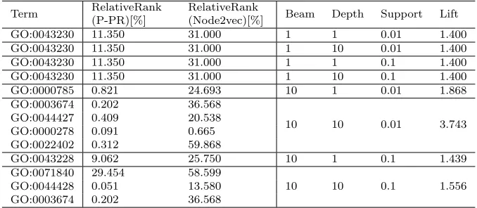
Table 3: The best rules discovered by the Hedwig algorithm on the breast cancer data set. The meaning of columns is the same as explained in the caption of Table 2.

Term RelativeRank (P-PR)[%]

RelativeRank

(Node2vec)[%] Beam Depth Support Lift

GO:0043230 11.350 31.000 1 1 0.01 1.400

GO:0043230 11.350 31.000 1 10 0.01 1.400

GO:0043230 11.350 31.000 1 1 0.1 1.400

GO:0043230 11.350 31.000 1 10 0.1 1.400

GO:0000785 0.821 24.693 10 1 0.01 1.868

GO:0003674 0.202 36.568

10 10 0.01 3.743

GO:0044427 0.409 20.538 GO:0000278 0.091 0.665 GO:0022402 0.312 59.868

GO:0043228 9.062 25.750 10 1 0.1 1.439

GO:0071840 29.454 58.599

10 10 0.1 1.556

GO:0044428 0.051 13.580 GO:0003674 0.202 36.568

percentiles of all term scores, giving credence to our hypothesis that high scoring terms are usually used in rules. On the other hand, use of the node2vec based scoring function was much less successful in this experiment.

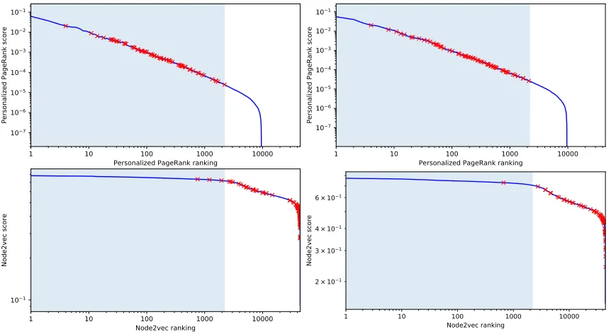
This phenomenon is clearly shown in the top two charts of Figure 4 showing all the terms used by Hedwig and their ranks. Even taking into account all (not only the best) rules, we see that predominantly the used terms come from the top 5 percent of all the terms as scored by the Personalized PageRank scoring function. On the other hand, this phenomenon does not occur with the node2vec scoring function, as the results in Table 2 and Table 3 show for the ALL and breast cancer data sets. The rules used by Hedwig score quite low according to the node2vec function, however as seen in the bottom two charts of Figure 4, the node2vec score of the used terms is still above average, and it is possible that the node2vec scores are useful. We consider the node2vec scores to contain sufficient information to warrant testing both scores in the second experimental setup.

The rules discovered in the first experimental setup are biologically relevant, except when the search beam for the Hedwig algorithm was set to 1. In this case the only significant rule discovered contained in its condition a single gene ontology term GO:0003674 that denotes molecular function. This is a very general term that offers little insight and shows that a larger search beam is necessary in order for Hedwig to make significant discoveries. The most interesting results are uncovered when the beam size is set to 10 and the support is

set to 0.01. When the depth is set to 1, the most important term GO:0050851 (antigen

(23)

1 10 100 1000 10000 Personalized PageRank ranking

107 106 105 104 103 102

Personalized PageRank score

1 10 100 1000 10000

Personalized PageRank ranking 107

106 105 104 103 102

1 10 100 1000 10000 Node2vec ranking

101 2 × 101 3 × 101 4 × 101

Node2vec score

1 10 100 1000 10000 Node2vec ranking

101 2 × 101 3 × 101 4 × 101

Node2vec score

Figure 4: The ranks of the terms used by Hedwig to construct rules on the ALL (left) and breast cancer (right) data sets. The blue line shows the score for each of the terms in the background knowledge—the scores on the top two charts were calculated with Personalized PageRank and the scores on the bottom two charts were produced with node2vec. The terms in each chart are sorted by descending score. Each red cross highlights one of the terms used by Hedwig. The blue area on the left denotes the top 5 percent of all nodes (i.e. nodes with a relative rank

of 0.05 or lower). Note the logarithmic scale of both axes.

5.1.2. Using Aleph

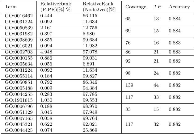
Tables 4 and 5 show the terms, used in the 10 best rules discovered by the Aleph algorithm that describe the ALL and breast cancer data sets, respectively, and the P-PR and node2vec

scores of the terms in the rules. The scores were calculated taking bothis-a and is-part-of

relations into account.

The results again show that the Personalized PageRank scoring function ranks all the terms used by Aleph remarkably high. Moreover, similar to the experiments with Hedwig, the node2vec scoring function is much less successful in this experiment. The high Person-alized PageRank ranking of terms appearing in rules discovered by the Aleph algorithm is also seen in Figure 5.

(24)

possible that the node2vec scores are useful. We consider the node2vec scores to contain sufficient information to warrant testing both scores in the second experimental setup.

5.2. Second setup: Shrinking the background knowledge ontology

This section presents the result of the second set of experiments with the NetSDM method-ology. We present the results of shrinking the background knowledge for Hedwig and Aleph.

5.2.1. Ontology shrinking for Hedwig

The results of the first experimental setup show that the scores, calculated using the network analysis techniques, are relevant to determine whether background knowledge nodes will be used by SDM algorithms in the construction of rules describing the target instances. Here we present the results of using the computed scores to shrink the background knowledge used by Hedwig. We first present the results of both scoring functions on the ALL data set and then on the breast cancer data set. We set the beam and depth parameters of Hedwig

to 10, and the minimum coverage parameter to 0.01; these are the settings that produced

the best results for both data sets in the first experimental setup with Hedwig with no shrinking of the background knowledge (see Tables 2 and 3).

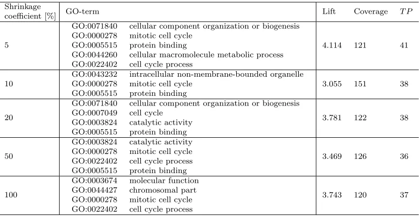
For Personalized PageRank-based network shrinkage we also test if taking into account edge directions makes a difference. Table 6 (undirected edges) and Table 7 (directed edges) show the results of semantic rule discovery using the P-PR function on the ALL data set. Both tables show a similar phenomenon: by decreasing the size of the background knowledge

1 10 100 1000 10000

106 105 104 103 102 101

1 10 100 1000 10000

106 105 104 103 102 101

1 10 100 1000 10000

Node2vec ranking 101

Node2vec score

1 10 100 1000 10000 Node2vec ranking

2 × 101 3 × 101 4 × 101 6 × 101

Node2vec score

(25)

Table 4: The 10 best rules discovered by the Aleph algorithm on the ALL data set. The meaning of the second and third column is the same as in Table 2. The scores

were calculated by taking theis-a and is-part-of relations into account.

Term RelativeRank (P-PR)[%] %

RelativeRank

(Node2vec)[%] Coverage T P Accuracy GO:0016462 0.444 66.115

65 13 0.884

GO:0031224 0.092 11.634 GO:0050839 2.161 12.756

69 15 0.884

GO:0031982 0.397 5.980 GO:0098609 0.855 99.684

76 16 0.883

GO:0016021 0.094 11.982

GO:0002703 4.948 97.078 86 21 0.883

GO:0030155 0.886 99.031

92 21 0.882

GO:0005634 0.056 6.891 GO:0031224 0.092 11.634

98 24 0.882

GO:0055114 0.184 99.827 GO:0050851 0.792 86.346

139 44 0.882 GO:0005488 0.009 94.384

GO:0044255 0.283 97.785

117 33 0.882 GO:1901615 1.030 99.553

GO:0006796 0.188 98.970

83 15 0.882

GO:0051129 3.045 97.949 GO:0007165 0.058 99.764

117 32 0.882 GO:0045321 0.622 92.021

GO:0044425 0.074 25.869

Table 5: The 10 best rules discovered by the Aleph algorithm on the breast cancer data set. The meaning of the columns is the same as in Table 4.

Term RelativeRank (P-PR)[%] %

RelativeRank

(Node2vec)[%] Coverage T P Accuracy GO:0022610 0.399 98.582

39 11 0.914

GO:0005578 1.041 13.932 GO:0050794 0.045 99.980

57 11 0.912

GO:0042592 0.435 93.017 GO:0044428 0.085 10.539

77 20 0.912

GO:0000226 1.243 80.543 GO:0043230 0.512 10.349

69 14 0.911

GO:0043087 0.969 80.674 GO:0044424 0.018 25.560

93 21 0.911

GO:0044843 2.028 53.978 GO:0044427 0.330 8.428

103 26 0.911 GO:0050790 0.227 99.147

GO:0008509 3.826 74.934

76 12 0.910

GO:0044699 0.047 99.996 GO:0005488 0.009 92.797 GO:0016491 0.289 99.942

86 14 0.910

GO:0080090 0.426 99.760 GO:0051186 1.227 97.193

84 13 0.910

GO:0043169 0.108 43.342 GO:0043226 0.029 17.895

97 19 0.910

GO:0004842 0.615 79.657

(26)

Table 6: Results of NetSDM using direct network conversion with undirected edges, Per-sonalized PageRank scoring function, na¨ıve node removal and the Hedwig SDM algorithm on the ALL data set.

Shrinkage

coefficient [%] GO-term Lift Coverage T P

5

GO:0002376 immune system process

GO:0002694 regulation of leukocyte activation GO:0034110 regulation of homotypic cell-cell adhesion

3.235 111 40 10

GO:0002694 regulation of leukocyte activation GO:0044459 plasma membrane part

4.090 90 41

20

GO:0003824 catalytic activity

GO:0044283 small molecule biosynthetic process GO:0044444 cytoplasmic part

4.257 116 55

50

GO:0002429 immune response-activating cell surface recep-tor signaling pathway

GO:0005886 plasma membrane GO:0005488 binding

3.420 105 40

100

3.420 105 40

50% still allows us to discover the same high quality conjunct of the terms GO:0002376, GO:0002429, GO:0005886 and GO:0005488 as before.

Comparing Table 6 and Table 7 we see that there is a slight difference in the resulting rules if we take the direction of the relations in the background knowledge into account. Better Lift values and more consistent results are obtained when we choose to ignore the direction of the relations. Taking edge directions into account, for example, leads to a

discovery of a very low quality rule with Lift value of only 2.219 when the background

knowledge is at 20% of its original size. When we do not ignore the direction of the

relations, the score of each node is only allowed to propagate to the ‘parent’ nodes in the background knowledge, i.e. high scores will be given to those GO terms whose child terms (specializations) have a high score. On the other hand, when ignoring the direction, we allow nodes to pass their high scores also to sibling nodes, allowing Hedwig in the final step of our NetSDM methodology (outlined in Algorithm 1) to choose the correct specialization of the parent node. More experiments are needed to analyze this phenomenon.

Table 8 and Table 9 show the results of the experiments using the node2vec function on the ALL data set. The results show that node2vec based ontology shrinkage did not achieve the same performance as the shrinkage using the Personalized PageRank function. The results in both tables show that lower shrinkage coefficients consistently decrease the quality of the rules discovered by Hedwig, meaning that shrinking of the background knowledge with the node2vec scoring function removes several informative terms and connections. Without these terms Hedwig could not extract the relevant information from the data, causing decreased performance.

(27)

Table 7: Results of NetSDM using direct network conversion with directed edges, Person-alized PageRank scoring function, na¨ıve node removal and the Hedwig SDM algo-rithm on the ALL data set.

Shrinkage

5

GO:0044238 primary metabolic process

3.741 132 55

10

GO:0044238 primary metabolic process

3.769 131 55

20

GO:0045936 negative regulation of phosphate metabolic pro-cess

GO:0009892 negative regulation of metabolic process

2.219 89 22

50

3.420 105 40

100

3.420 105 40

Table 8: Results of NetSDM using direct network conversion with undirected edges,

node2vec scoring function, na¨ıve node removal and the Hedwig SDM algorithm on the ALL data set.

Shrinkage

5 GO:0050852 T cell receptor signaling pathway 2.586 125 36 10 GO:0050852 T cell receptor signaling pathway 2.586 125 36 20 GO:0050852 T cell receptor signaling pathway 2.586 125 36 50 GO:0050863 regulation of T cell activation 3.076 108 37 100

3.420 105 40

returning a single GO term as the only important node. This may be a consequence of so many terms pruned that the remaining terms describe non-intersecting sets of enriched genes (or sets with a very small intersection). In this case, term GO:0044281 covers the largest number of instances and is therefore selected as the best term. Upon selecting this term, Hedwig is not able to improve the rule by adding further conjuncts, as adding any other term to the conjunction drastically decreases the coverage of the resulting rule.