Monotone Learning with Rectified Wire Networks
Veit Elser [email protected]
Department of Physics Cornell University
Ithaca, NY 14853-2501, USA
Dan Schmidt [email protected]
and Jonathan Yedidia [email protected]
Analog Devices, Inc. Boston, MA, USA
Editor:Samy Bengio
Abstract
We introduce a new neural network model, together with a tractable and monotone online learning algorithm. Our model describes feed-forward networks for classification, with one output node for each class. The only nonlinear operation is rectification using a ReLU function with a bias. However, there is a rectifier on every edge rather than at the nodes of the network. There are also weights, but these are positive, static, and associated with the nodes. Ourrectified wire networks are able to represent arbitrary Boolean functions. Only the bias parameters, on the edges of the network, are learned. Another departure in our ap-proach, from standard neural networks, is that the loss function is replaced by a constraint. This constraint is simply that the value of the output node associated with the correct class should be zero. Our model has the property that the exact norm-minimizing parameter update, required to correctly classify a training item, is the solution to a quadratic pro-gram that can be computed with a few passes through the network. We demonstrate a training algorithm using this update, called sequential deactivation (SDA), on MNIST and some synthetic datasets. Upon adopting a natural choice for the nodal weights, SDA has no hyperparameters other than those describing the network structure. Our experiments explore behavior with respect to network size and depth in a family of sparse expander networks.
Keywords: Neural Networks, Online Training Algorithms, Rectified Linear Unit
Some of the simplest modes of machine learning are monotone in character, where the representation of knowledge changes unidirectionally. In the k-nearest-neighbor classifica-tion algorithm (Cover and Hart, 1967), for example, exemplars of the classes are amassed, monotonically, over the course of training. It is also possible to have monotone learning where memory does not grow, but decreases over time. Suppose we try to classify Boolean feature vectors using conjunctive normal form formulas, one for each class. Starting with large and randomly initialized formulas, during training we simply discard, from the for-mula of the feature vector’s class, all the inconsistent clauses (Mooney, 1995). Clearly an attractive feature of both of these monotone algorithms is the computational ease of reach-ing the desired outcome, i.e. additional exemplars for improved discrimination, or discarded clauses to better accommodate a class.
c
We report on a new kind of monotone learning where during training only the values of a fixed number of parameters are changed, and in a monotone fashion. Like the two examples above, there is a simple and computationally tractable objective when learning each new item. But perhaps the most interesting feature of our scheme is that it operates on deep networks of rectifiers, a setting where training is not normally seen as computationally tractable.
Monotone learning with deep rectifier networks is made possible by two changes to the standard paradigm: (i) conservative updates that minimize the norm of the parameter changes, and (ii) eliminating all but the bias variables as learned parameters.
Although the feedforward computations in standard neural network models are inspired by biological neuronal computations, the training protocols in widespread use seem far from natural. Humans are able to generalize the shape of the digit 5 without suffering through many training “epochs” through a data set, and are capable of building a rudimentary repre-sentation of digits or other classes of objects from relatively few examples. The conservative learning principle, introduced to the best of our knowledge by Widrow et al. (1988) as the “minimal disturbance principle,” comes closer to our experience of natural learning. In this mode of learning the parameters of the network are minimally changed to accommodate each example as it is received, with the rationale that the attention to minimality preserves the representation created by earlier examples.
The minimal disturbance principle was reprised by Crammer et al. (2006) as the “passive-aggressive algorithm”, in the context of support-vector machines. There are relatively few models where “aggressive” parameter updates — minimal, yet achieving immediate results — are easily computed. To emphasize the norm-minimizing characteristic of this learning mode we use the term “conservative learning.” An approximate implementation of conser-vative learning was successfully used to discover the Strassen rules of matrix multiplication (Elser, 2016).
In the present work we make changes to the “standard neural network model” to enable conservative learning. In broad outline, the changes guarantee monotonicity, making the computation of the conservative updates tractable. A key step was elevating the role of the additive parameter, or bias. The metaphor that replaces Hebbian synapse (weight) learning is that of a silting river delta, with myriad channels whose levels (bias) rise differentially, but monotonically, over time.
Below is an overview of our contributions.
• Inspired by analog implementations of logic, we propose replacing the conventional rectified sum computed by a standard neuron using a ReLU function
y←max 0, X
i
wixi−b
!
,
by a sum of rectifications:
y←wX
i
max (0, xi−bi). (1)
• Even with just positive weightsw in (1), we show that networks ofrectified wires can represent arbitrary Boolean functions. This construction makes use of doubled inputs, where true is encoded as (1,0), false as (0,1), and generalizes, for symbolic data, to one-hot encoding.
• The node values of our networks are non-negative. We propose defining class mem-bership of data by the corresponding output node having value zero.
• Because the biases on all the wires are non-negative and can only increase during training, we choose to initialize them at zero.
• We show that the 2-norm minimizing change of the bias parameters, that sets the class output node for a given input to zero, is the solution to a quadratic program.
• An iterative algorithm similar to stochastic gradient descent, including both backward propagation and a new kind of forward propagation, is proposed to approximately find the 2-norm minimizing bias changes. Executing the minimum number of iterations required to make the class output node the smallest in value defines the sequential deactivation algorithm (SDA).
• We show that a particular limit of SDA, on networks with a single hidden layer, learns arbitrary Boolean functions.
• Networks with better scaling have multiple layers, and their training is sensitive to the settings of the static weights. We propose balanced weights based just on the in-degrees and out-degrees in this general setting.
• A two-parameter family of random sparse expander networks is introduced to explore the size and depth behavior of learning in our model.
• Conservative learning on rectified wire networks with the SDA algorithm is demon-strated for MNIST and synthetic datasets.
• Despite our model’s capacity for depth in its representations, we find that the best experimental results with the SDA algorithm are obtained in a limit where deactiva-tion occurs only in the final layer, where the model is equivalent to a network with just a single hidden layer of rectifier gates. The pursuit of conditions that fully utilize activation/decativation in all layers is identified as the goal of future research.
1. Rectified wire networks
One motivation for our network model is the implementation of logic by analog computations without multiplications. The analog counterparts of true and false are, respectively, the numbers 1 and 0. Before presenting our “rectified wire” network model, we consider networks constructed from biased rectifier gates. A biased rectifier gate with K inputs,
generalizes and and or gates. and gates are realized with biasb =K−1. We would get theorgate with b= 0 if we could saturate the output at the value 1. We show below how this detail can be fixed with additional rectifiers and a suitable network design.
Negations are completely absent from our rectifier implementations of general logic circuits. This is made possible by the process of demorganization, where not gates are pushed through the circuit from output to input, exchangingandand orgates as dictated by De Morgan’s laws. After all thenotgates have been pushed through, the only remaining not gates act directly on the inputs. We accommodate this by allowing each input to the logic circuit to be replaced by an analog pair with values (1,0) fortrueand (0,1) forfalse. We refer to this encoding scheme as input doubling.
It is relatively straightforward to show, as we do in theorem 1.1, that networks com-prising only rectifier gates, with bias variables as the only parameters, can mimic any logic circuit. From the machine learning perspective, our network model has at least the capacity to represent the classes defined by the truth value of arbitrary Boolean functions. However, the parameter settings that realize these Boolean classes are very special points in the con-tinuous parameter space of the model, and are not claimed to be directly relevant for the intended use of these networks.
Theorem 1.1 Any Boolean function on N inputs and computed with M binary and/or
gates and any number of not gates can be implemented by an analog network comprising
at most5M biased rectifier gates taking the corresponding 2N doubled analog inputs.
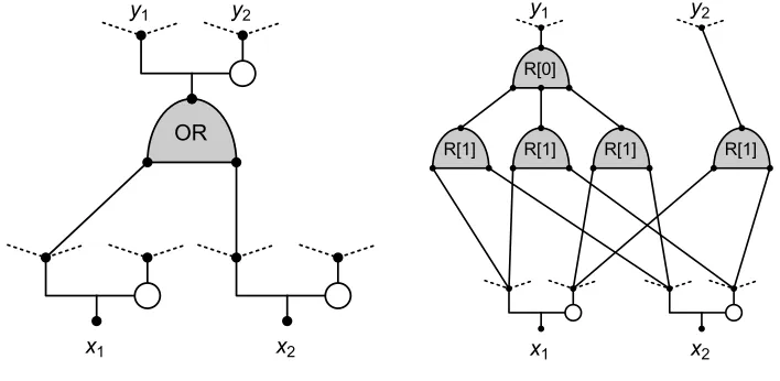
Proof As a circuit, the function takesN Boolean inputs and produces one Boolean output. We associate negations in the circuit with gate outputs as shown for the case of the and gate in the left panel of Figure 1. Upon output, both the gate output y1 and its negation y2 by anot gate (rendered as an open circle), are made available to gates receiving inputs.
One of the output forks might not be used, as for the final gate of the circuit whose single output is the value of the Boolean function. The diagram also shows how each of the gate inputs is derived from one fork of the output of another gate, or an input to the circuit.
The body of the proof consists of confirming that the Boolean gate relationship between the inputs (x1, x2), and the output y1 and its negation y2, is exactly reproduced by a
corresponding rectifier gate network. The replacement for the and gate is shown in the right panel of Figure 1. All bias parameters are either 0 or 1, and the only values that arise on the nodes are also 0 and 1. The replacement rule for the or gate is shown in Figure 2. For both of the circuit replacement rules just described there are three others, where one or both of the inputs are negated. These are trivially generated from the ones shown by inserting a negation right after the inputs (x1 or x2 or both), which is equivalent to
swapping the branches of the input-forks.
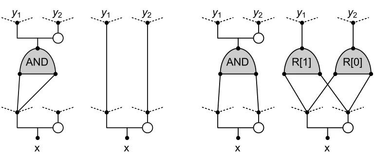
Figure 1: and gate and its replacement with rectifier gates in the analog network.
Figure 2: or gate and its replacement with rectifier gates in the analog network.
The only negations remaining after all and and or gates have been replaced are those in the N input forks to the circuit. These are taken care of by defining the input to the analog network as the 2N values on the branches of those forks. The resulting network will have only rectifier gates. From the gate replacement rules (Figs. 1-3) we see that the number of rectifier gates is at most 5M.
Figure 3: and gate replacement rules when both inputs come from the same output fork, either the same branch (left) or both branches (right). The rule for theor gate is the same for the case on the left, and hasR[0] andR[1] exchanged for the case on the right.
We give these biases the freedom to take different values, increasing the expressivity of the network and boosting the parameter count commensurate with “standard model” networks, which have a weight on each edge. By setting the biases on selected edges in a completely connected network to large values, thereby disabling them, our model has the capacity to select its architecture.
The second way we generalize the model is to introduce weights at all the summations. These are static — not intended to be learned — and positive. We show in section 6 that in layered networks one can apply a rescaling to the biases that has the effect of restoring all the weights to 1 without changing the classification behavior of the network. The weights therefore only play a role during training, through the gain/decay they impart to the analog signal as it propagates from input to output, and the response this elicits from the bias parameters.
We now formally define our model.
Definition 1.2 A rectified wire network is a model of computation on a directed acyclic graph. Associated with each wire or edgei→j joining nodeito j is the node value xi and
edge output yi→j related by
yi→j = max (0, xi−bi→j),
where bi→j is the bias parameter for the edge. The edge outputs yi→j, from all edges i→j
incident on node j, are summed to give the value xj of node j:
xj =wj
X
i→j
The positive constantwj is the weight of the node. The node valuesx, edge outputs y, and
bias parameters b of a rectified wire network are general real numbers.
The number of edge outputs ysummed by a node jis its in-degree |→j|, and the number of edges receiving xj as input is its out-degree |j→|. Nodes with in-degree zero are input
nodes and have their x values assigned. The outputs of the network are the x values of the nodes with out-degree zero, the output nodes. Nodes which are neither input nor output nodes are the hidden nodes of the network. The connectivity of rectified wire networks is such that there always exists a path between any input node and any output node.
The content of theorem 1.1, re-expressed in terms of rectified wires, takes the following form:
Corollary 1.3 The truth value of a Boolean function on N variables that can be computed with M binary and/or gates and any number of not gates can be represented by a
two-output rectified wire network taking2N doubled inputs and having at most7M hidden nodes. Like the doubled inputs, the two output nodes encode the truth of the function with values
(1,0)or (0,1).
Proof A logic circuit with M binary and/or gates has M nodes, one at each gate out-put. When re-expressed as a rectified wire network, each gate output is replaced by two nodes and, in the worst case (Figs. 1-2), the gate itself results in five additional nodes. The number of hidden nodes in the resulting rectified wire network is therefore bounded by 7M. The wiring of the nodes, including the input and output nodes, can be the complete acyclic graph because large bias settings, by deselection, realize any network on the given number of nodes.
While possible in principle, we should not expect it to be easy for a rectified wire network to learn bias values on the modest networks promised by corollary 1.3 when presented with data generated by a Boolean function. On the other hand, as we show in section 3, this particular network model has a significant advantage over the “standard model” in having tractable conservative learning. A different, equally valid representation might be learned instead, most likely on a much larger network.
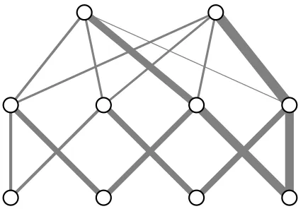
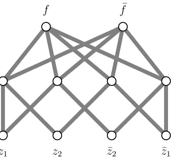
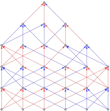
We render rectified wire networks as simple directed graphs, with input nodes at the bottom, output nodes at the top, and all edges directed in the upward direction. The rendering of the bias values — the only learned parameters — is through the edge thickness. Edges with low bias are thick, those with high bias are thin. When the bias on an edge is so great that the rectified value is zero for any input to the network, the edge is effectively absent (zero thickness). Figure 4 shows this style of rendering of a network with four input, four hidden, and two output nodes.
We can generalize both the inputs and the outputs of rectified wire networks to expand their scope beyond Boolean function-value classifiers. In many applications the feature vectors are strings of symbols from a finite alphabet: {true, false},{a,c,g,t}, etc. As in the Boolean case, for an alphabet of sizeK we use the one-hot encoding scheme where the
Figure 4: Rectified wire network with four input nodes (bottom row), four hidden nodes, and two output nodes (top row). Thinnest edges have the highest bias.
each component i= 1, . . . , L over the dataset. The data vector for input to the network, corresponding tov, is then
d(v) = [θ1(v1),1−θ1(v1), . . . , θL(vL),1−θL(vL) ]. (2)
With this convention, the input to the network is always a vector of numbers between 0 and 1 whose sum equals the number of components or string length of the data. The mapping by the cumulative probability functions, in the case of analog data, ensures that the distribution in each channel is uniform.
The number of output nodes equals the number of data classes. A Boolean function classifier would have two output nodes to classify the truth value of the input. To classify MNIST data (LeCun et al., 1998), the network would have 10 output nodes. Before we describe how these outputs are interpreted we make a trivial observation:
Lemma 1.4 In a rectified wire network with input vector d≥0, there exist settings of the bias parameters where, for any of the output nodes c ∈C, we have xc= 0 and xj >0 for
j∈C\ {c}.
Proof All the output nodes will have positive values for zero bias, because the weights are positive and each output is connected by a path to one of the inputs with positive value (see definition 1.2). To exclusively arrange for xc = 0, we set bi→c = xi on all the edges
i→c incident onc(keeping all other biases at zero).
We will explain in section 3 why zero is the appropriate indicator function value for defining classes on a conservatively trained rectified wire network.
2. Notation
network. These bear a latin index when defined on a node of the network. Examples are the node values, xi, or the weights wi. The index is written as a directed edge between
nodes when defined on an edge of the network. Examples are the bias parameters, bi→j,
and edge-outputs yi→j. The same lower case symbols, both for nodes and edges, when
written without subscripts denote the vector of all the indexed values. For example, b is the vector of all biases in the network and dthe vector of data values on the input nodes. When such symbols appear in an equality/inequality, the relation applies componentwise. Round brackets attached to a variable identify its functional dependence, when relevant. The value of nodek, for example, might be writtenxk(b, d) to emphasize its dependence on
the biases and input data.
Upper case symbols are used for sets. The symbols D, H,C are reserved for the data (input), hidden, and class (output) nodes respectively, whileE is the set of directed edges. Upper case symbols are also used for continuous sets with the same convention for functional dependence as variables. For example,B(d) might be the set of bias values bsuch that for
b ∈ B(d) the node value xi(b, d) is zero for input d. Cardinality is denoted with vertical
bars, e.g. |E| for the number of edges in the network. Node iin a network has in-degree
|→i|and out-degree|i→|.
3. Counterfactual classification and conservative learning
Monotone learning on rectified wire networks is made possible by the fact that, for a fixed input d ≥ 0 to the network, the value xk(b, d) at any node k is a negative and
non-increasing function of the bias parametersb. This, combined with the fact (lemma 1.4) that zero is always a feasible value on any of the output nodes, motivates the following definition of a classifier.
Definition 3.1 The output nodes C of a rectified wire network serve as a classifier of |C| classes of inputs when there are biases b such that for inputs din class c∈C, xc(b, d) = 0
and xi(b, d)>0 for i∈C\ {c}.
To see why this definition makes sense in the context of conservative learning, suppose that at some stage of training all the output nodes are positive for some inputdin classc. By increasing the biases b, the output valuexc(b, d) can always be driven to zero for input
d, and by increasing them as little as possible, i.e. conservatively, there is a good chance the other output nodes can be kept positive. If some of the other outputs are also set to zero in the process of increasing biases, the classification is ambiguous. In any case, and after any amount of subsequent training where biases are increased, monotonicity ofxc(b, d) with
respect tob ensuresxc(b, d) = 0 continues to be a valid indicator for class c.
The outputs of the proposed classifier are counterfactual in the sense that a large positive value xc on the node for class c represents strong evidence that c is not the correct class.
In the case of a class defined by the truth value of a Boolean function, we would use the function that returns false for members of the class, so the value of the corresponding analog circuit output node is zero.
Definition 3.2 The cost, in a rectified wire network, for changing the biases from b to b0, is the p-norm kb0−bkp.
The uniqueness of the cost-minimizing bias change, for fixing a misclassification, depends on the norm exponentp. We mostly usep= 2 in this study, where uniqueness can be proved. Our definition of the conservative learning rule, which sidesteps uniqueness, is the following:
Definition 3.3 Suppose output node c∈C for class c has value xc(b, d) >0 for an input
d, in a network with biases set at b. A conservative bias update is any b0 that minimizes kb0−bkp and produces output valuexc(b0, d) = 0.
Lemma 3.4 If b0 is any conservative update of b, then b0 ≥b.
Proof Biases b0 have just learned an input din some class c ∈ C, soxc(b0, d) = 0. Now
suppose b0i→j < bi→j for some edgei→ j ∈E. The update b00, where b00i→j =bi→j and all
others are unchanged, has lower cost than b0 and yet, by monotonicity of node values with respect tob, all output nodes with value zero will still be zero, including xc(b00, d).
The outputs of a rectified wire network are compositions of rectifier functions. Com-position of convex functions are in general not convex, but for the rectifier function this is true. We give an inductive proof based on the following.
Lemma 3.5 If x(b) :RK →R is convex, then y(a, b) : (R,RK)→R, defined by y(a, b) = max (0, x(b)−a),
is also convex.
Proof Because x is convex, for arbitraryb1, b2∈RK we have
x(λb1+ (1−λ)b2)≤λ x(b1) + (1−λ)x(b2) (3)
for 0≤λ≤1. For arbitrarya1, a2 ∈R, y(λa1+ (1−λ)a2, λb1+ (1−λ)b2)
= max (0, x(λb1+ (1−λ)b2)−λa1−(1−λ)a2) ≤max (0, λ x(b1) + (1−λ)x(b2)−λa1−(1−λ)a2)
= max (0, λ z1+ (1−λ)z2),
where we have used (3) and defined
z1 =x(b1)−a1 z2 =x(b2)−a2.
Since for arbitrarys, t∈R
we obtain
max (0, λ z1+ (1−λ)z2)≤max (0, λ z1) + max (0,(1−λ)z2)
=λmax (0, z1) + (1−λ) max (0, z2)
=λ y(a1, b1) + (1−λ)y(a2, b2)
as claimed.
Theorem 3.6 The node values x(b, d) of a rectified wire network, given an input d, are convex functions of the bias parameters b.
Proof The values of the input nodes D, set to the constant values xi = di, i ∈ D, are
trivially convex. Since our network is an acyclic graph, the nodes can be indexed by consecutive integers so that all edge outputs yi→j incident on a node j ∈H∪C are from
input nodesi∈Dor from hidden nodesi∈H that havei < j. For any j∈H∪C, we use induction and suppose allxi,i∈H withi < j are convex functions of the bias parameters.
Consider any of the edge outputsyi→j(b) incident on j:
yi→j(b) = max (0, xi(b)−bi→j).
Seen as a function of bias parameters, wherexi(b) is a convex function of biases not including
bi→j,yi→j(b) fits the hypothesis of lemma 3.5 and is therefore convex. This conclusion also
applies to the base case, the hidden node numberedj= 1, where all thexi are inputsi∈D
and constant. Since the node value
xj(b) =wj
X
i→j
yi→j(b)
is a positive multiple of a sum of convex functions, it too is convex and completes the in-duction.
For the case p= 2, we can prove uniqueness of the conservative bias update.
Corollary 3.7 The set B(d), of biases b of a rectified wire network with fixed input d for which xc(b, d) = 0 for a given output node c, is non-empty and convex. Consequently, the
conservative bias updateb0 ∈B(d)that minimizes the cost kb0−bk2 with respect to the biases b is unique.
Proof The setB(d) may be defined as the feasible set ofxc(b, d)≤0 (since this function is
non-negative). By lemma 1.4B(d) is non-empty, and by theorem (3.6)B(d) is closed and convex because xc(b, d) is a convex function of b. Now suppose b01 ∈ B(d) and b02 ∈ B(d)
are distinct minimizers of kb0 −bk2 for some bias b. Because B(d) is convex we have a
To design algorithms for computing the conservative bias update and to establish the complexity of this task we cast the problem as a mathematical program. Consider a rectified wire network with edges E on which we are given bias parameters b, say from previous training. Suppose we now wish to learn the pair (c, d), a vector of input data d in the class associated with output nodec. Unless xc(b, d) = 0, the biases must be conservatively
updated to b0 so this is true. Before we do this we partitionE into the set ofactive edges
A and its complement, ¯A.
Definition 3.8 The set A of active edges of a rectified wire network, given input data d and bias parameters b, are those edges i→ j where xi(b, d) > bi→j, or equivalently, where
yi→j(b, d)>0.
The biasesbi→j on the inactive edgesi→j∈A¯, when increased, have no effect on any
node values, in particular the output nodes, because the corresponding edge-outputs yi→j
are zero by monotonicity of x(b) (non-increasing). To find b0 we may therefore work with the network induced by the active edgesA, called the “active network.”
Our mathematical program makes use of a set of reduced bias variables.
Definition 3.9 Let A be the active edges of a rectified wire network for input data d and bias parameters b. For each edge i→j of the network, define the reduced bias by
b−i→j =
bi→j, i→j ∈A
xi(b, d), i→j ∈A.¯
Now consider a conservative updateb0 ofb, and the reduced biasesb−forb0. We always have
b− ≤b0, and the reduced values have the property that x(b−, d) = x(b0, d). In particular, for the class output node c we have xc(b−, d) = xc(b0, d) = 0. The only reason that a
conservative update b0 of b would not already be reduced (b0 = b−) is that the freedom
b−≤b0 may allow a reduction in cost, that is, give a more conservative update.
We now define the mathematical program. For given data d, biasesb and weightsw on a rectified wire network, we are given the corresponding active edges A and node c of the correct class. The unknowns are the updated biasesb0, reduced biasesb−, and edge-outputs
y on A, and the values ofx on cand the input and hidden nodes:
minimize: kb0−bkp
p (4a)
such that: b−≤b0, (4b)
0≤b−, (4c)
xi=di, i∈D (4d)
yi→j =xi−bi−→j, i→j ∈A (4e)
0≤yi→j, i→j ∈A (4f)
xj =wj
X
i→j∈A
yi→j, j∈H∪ {c} (4g)
Theorem 3.10 The mathematical program (4), defined for the networkAthat is active for given biasesb and data d, as part of its solution b0 gives a conservative bias update for the class associated with output node c.
Proof First observe that any valid (xc= 0) assignment of node valuesx and edge-outputs
y, in the corresponding rectified wire network, is realized by a feasible point of the linear system (4c) – (4h) involving just the reduced biases (notb0). For the variablesb0 to be recti-fied wire biases consistent with the reduced biasesb−, it is sufficient for them to satisfy (4b), as monotonicity ensures xc(b0) = 0. Optimizing (4a) subject to (4b) and the constraints
that define the feasible set of reduced biases, gives the most conservative update.
For p = 2, (4) is a positive semi-definite quadratic program and can be solved in time that grows polynomially (Kozlov et al., 1980) in the size of the active network, |A|. The same conclusion applies forp= 1, a linear program, because the objective can be replaced by the sum of all the updated biases b0 provided we impose the result of lemma (3.4),
b ≤b0, as a constraint. While these results allow us to add rectified wire networks to the list of models for which there is a tractable conservative learning rule, in most applications it is also important that training scales nearly linearly with the size of the network. The
sequential deactivation algorithm (SDA) described in the next section is designed to meet that goal.
We close this section by reviewing the features of our model that make training tractable. The insistence on exactly learning individual items should not be counted as a tractability-enabling feature. Indeed, it is easy to see how the mathematical program (4), to compute the conservative update for one data item, would be generalized to find the norm-minimizing update that classifies an entire mini-batch. All the variables and data, with the exception of the biasesbandb0, now carry a data indexm∈M, whereM is a mini-batch. For example, (4b) would be replaced by
b−i→j,m≤b0i→j i→j∈A, m∈M
and imposes consistency of the bias updates for all instantiations of the reduced biases over the mini-batch. While the size of the mathematical program has grown toO(|A||M|) equations and inequalities, it is still tractable.
Convexity of the variables x and y with respect to the bias parameters is clearly im-portant for tractable learning, and the proofs of lemma 3.5 and theorem 3.6 show that this relies on the non-negativity of the static weights and the form of the activation function. Less obvious in facilitating tractability is the proposal to replace the loss function of neural networks by a constraint, and in particular, the simple constraint (4h). For example, one might consider replacing this single constraint with the following set of inequalities,
xi > xc+ ∆, i∈C\c, (5)
where the fixed positive parameter ∆ specifies a margin for avoiding ambiguous classifi-cation. After all, we still have a tractable mathematical program after this substitution. Unfortunately, this proposal creates a conflict in the relationship between the reduced biases
inequality b− ≤ b0 to preserve this constraint when b− biases are replaced by b0 biases in the rectified wire model (the monotonic decrease of a non-class output may exceed that of the class output).
4. Sequential deactivation algorithm
This section describes in detail the SDA algorithm for computing bias updates in the rectified wire model. While these updates are not guaranteed to be the most conservative possible, their computation is significantly faster than solving a general quadratic program. The SDA algorithm resembles the gradient methods used for optimizing standard model networks, the most widely used being stochastic gradient descent (SGD) (Rumelhart et al., 1986).
The program (4) would be greatly simplified if inequality (4f) was somehow automati-cally satisfied. All active edges would remain active in the update and the updated biases
b0 on them would be equal to the reduced biasesb−. The node variablesx, in particularxc,
would be linear functions of the b0:
xc(b0) =xc(b) +∇xc·(b0−b).
For the p= 2 norm on bias updates, the optimal update that achievesxc= 0 is then
b0 =b− xc(b) k∇xck2
∇xc.
The conservative update, in this simplification, is the same as gradient descent.
In the general case, where edges may become inactive, from the monotonicity of xc we
know at least that the gradient∇xcnever has positive components. If we had the stronger
property, that ∇xc is also never zero while xc > 0, then gradient descent will always find
an update b∗ that satisfies xc(b∗) = 0. But the latter property follows immediately from
the fact thatxc>0 is only possible when there are active edges incident to output nodec,
so that xc has non-zero derivatives at least with respect to the biases on them.
While gradient descent cannot guarantee the norm minimizing update promised by the solution of program (4), it has some attractive features. First, the computation of the (piecewise constant) gradient is fast, as is the computation of the step size to the next gradient discontinuity (deactivation event). Second, there is an opportunity to make the gradient descent update b∗ more conservative on the inactive edges. Using the condition
yi→j(b∗) = 0 as the indicator of an inactive edge, the improved update is, for alli→j∈A,
b0i→j =
max (bi→j, xi(b∗)), yi→j(b∗) = 0
b∗i→j, yi→j(b∗)>0. (6)
The SDA algorithm is the efficient implementation of gradient descent on the rectified wire model followed by (6). Its name draws attention to the fact that the steps in the descent are defined by deactivation events.
Algorithm 1 Elementary network procedures
procedure eval(E,b,d) →(A, x, y)
xi ←di, i∈D
xj ←wjPi→j∈E yi→j, j∈H∪C
yi→j ←max(0, xi−bi→j), i→j ∈E
A← {i→j∈E:yi→j = 0}
end procedure
procedure grad(A,c)→ ∇xc
(−∇xc)j ←wcδjc, j ∈C
(−∇xc)i←wiPi→j∈A(−∇xc)j, i∈H
end procedure
procedure velocity(A,∇xc) →y˙
(−y˙)i→j ←(−∇xc)j+wi
P
k→i∈A(−y˙)k→i, i→j∈A
end procedure
the class. In addition to the output node values {xi :i∈C}, evalalso provides the edge
outputsy and the set of active edgesA (on which the edge outputs are non-zero).
Suppose the current bias parameters are b(0). Denote by (−∇xc)i→j the negative
gra-dient component for the bias on edge i→ j ∈ A. Because the derivatives with respect to all the bi→j on active edges into the same node j are equal, the node-indexed variables
(−∇xc)j := (−∇xc)i→j, i→j∈A
are well defined. In particular, if j is an output node, then (−∇xc)j =wcδjc. As long as
the gradient is constant, the biases evolve as
bi→j(t) =bi→j(0) +t(−∇xc)j, (7)
wheret is a continuous “time”.
The gradient (−∇xc)i is positive only if node iis connected by active edges to nodec,
with value given by the sum over all paths on active edges, each contributing by the product of weights along the path. The effect onxc of a bias change on an active edge into iis the
same as if the same bias change was instead applied to all the active edges leaving node i, but multiplied bywi. This implies the recursion,
(−∇xc)i =wi
X
i→j∈A
(−∇xc)j, i∈H (8)
in the proceduregradof Algorithm 1 and corresponds to back propagation in the network. The third procedure, velocity, is derived from the recursion for the edge-outputsy:
yi→j =wi
X
k→i∈A
Taking the time derivative and using (7),
(−y˙)i→j =wi
X
k→i∈A
(−y˙)k→i+ (−∇xc)j (9)
we obtain the velocities of the edge-outputs by forward propagation. The initialization occurs at edges i → j from all the input nodes i, for which the sum in (9) is absent and (−∇xc)j is set by grad.
By construction, bothyi→j(0) and the (constant) velocities (−y˙)i→j on the active edges
i→j∈Aare positive and the first deactivation event occurs at time
t∗= min
i→j∈A
yi→j(0)
(−y˙)i→j
. (10)
This is the time step in one iteration of the SDA algorithm. After the biases are incremented by (7) and the newly deactivated edges are removed from A, another round is begun. Iterations are terminated when eval returns xc = 0. The final biases are obtained by
applying (6) to the gradient descent biases.
We now revisit the classification rule of definition 3.1, where data is declared learned when xc = 0. Recall that this has the desired property of not having the “supremacy”
(smallest value among all classes) of node c spoiled by subsequent training. The only way that the latter can have a negative effect, through the general decrease in output values with increasing biases, is when output nodes other than c are in a tie at value zero. To mitigate this effect, and also make the bias changes even more conservative, we introduce theultra-conservative learning rule:
Definition 4.1 In the ultra-conservative mode of learning with the SDA algorithm,
itera-tions are terminated when xc, the value of the output node c of the correct class, is either
zero or smaller than the values of all the other output nodes.
This termination criterion is conservative from the point of view of testing. Consider the early stages of training, when we might want to test the algorithm on which class is being favored. The natural candidate for the latter is the output node with the smallest value. By terminating sda as soon as this criterion is met, the test (when performed right after training) will succeed with a smaller change to the biases than is required by the xc = 0
criterion.
Because the property of data d producing the smallest output value on nodec can be spoiled by training with datad0 6=d, it may be necessary for the network to retrain ond, or data similar to d, in order to properly learn the combination (d, c). The implied heuristic is that the net bias change for this mode of learning classcmay be more conservative than always insisting on outputxc= 0 for everydin this class.
The sda algorithm with the ultra-conservative termination criterion is summarized in Algorithm 2. As soon as xc becomes the smallest output or is zero, the algorithm returns
Algorithm 2 Sequential Deactivation (SDA)
input (E, b0),(d, c) (network edges, initial biases), (data vector, class)
b←b0 initialize biases
(A, x, y)←eval(E, b, d) active edges, node and edge output values
iter←0 zero the iteration counter
while xc>0 and arg mini∈Cxi 6={c} do iterate until nodecis smallest
∇xc←grad(A, c) gradient with respect to active biases
˙
y←velocity(A,∇xc) edge output velocity
t∗←mini→j∈A yi→j/(−y˙i→j) step size
fori→j ∈A do
bi→j ←bi→j+t∗(−∇xc)j increase biases
end for
(A, x, y)←eval(A, b, d) new active edges, node and edge output values
iter←iter+ 1 increment iteration counter
end while for i→j∈E do
if i→j∈A then
b0i→j =bi→j keep biases on active edges
else
b0i→j = max(b0i→j, xi) conservative update for inactive edges
end if end for
output b0,iter updated biases, iteration count
termination rule. Empirically (section 9) we find the number of iterations is often quite small and depends only weakly on network size. A second effect, serving to lessen the work, is the sparsification of the active network with time. In any event, the total computation in learning each data item would be at most O(|A|2), since in each iteration at least one of
the active edges is deactivated (and eliminated from subsequent rounds).
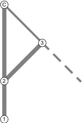
Figure 5: A network fragment on which the SDA update is not optimal. The initial bias on the thick edges is zero, while b3→c = b. Another parameter is the weight w
of node 2; all other nodes have unit weight. The dashed edge is inactive initially and irrelevant, but was responsible forb >0 from prior training.
accounts for the positive bias b3→c = b. The nodes all have unit weight except node 2,
whose weight is w. Data vector component d1 = 1 (on node 1) is the only one relevant for
the fragment shown.
It is easy to see that for the casew < bthe SDA solution is optimal, that is, it coincides with the solution of (4). However, with a bit of work one can show that the SDA updates are suboptimal when w > b, even when taking advantage of (6). This example only shows there is room for improvement. We do not know how pervasive this type of instance is in practice, let alone how seriously it impacts learning.
We close this section with the observation that SDA is not that different from SGD applied to the loss functionxc. The main differences are that the step size (learning rate) is
not a free parameter but set by deactivation events and that multiple steps may be executed when learning each data item. The benefit imparted by the rectified wire model, in this context, is just that the gradient computations and step sizes are very easy to compute. If we set aside monotonicity and solution guarantees, these attributes carry over to loss functions that are much stronger thanxc.
To get a sense of how small a change moves the model into difficult territory, consider the problem of learning the truth value of a Boolean functionf(z) onN variables generated by
M binaryand/orgates, as discussed in section 1. The rectified wire network would receive 2N doubled inputs and have output nodes f and ¯f, trained so that (xf, xf¯) = (f(z),f¯(z)).
having at most 7M hidden nodes. The outstanding question, of course, is whether a gradient based algorithm can find the appropriate bias settings.
Instead of the monotone loss function xf(z), fraught with the problem that training
cannot prevent (xf, xf¯) = (0,0) — an ambiguity — we might try the hinge-loss function
max
0, xf(z)−xf¯(z)+ ∆
.
By corollary (1.3) we know that it is possible to achieve zero loss over all z with margin ∆ = 1, and that the data will be correctly and unambiguously classified. Like xf(z), this
loss function is piecewise linear on the rectified wire model and can likewise benefit from fast gradient and step size calculations. Because this loss is no longer monotone decreasing in the bias parameters, there is now no reason to initialize biases at zero. The loss of monotonicity, of course, brings with it the zero gradient problem. We suspect this may be more serious for rectified wires than it is in standard network models.
5. Clause learning
Although the SDA algorithm provides a tractable computation for learning individual data in the rectified wire model, we do not yet have any reason to believe this algorithm can learn any interesting functions. To address that concern, in this section we show that at least in a particular limit, the SDA algorithm is able to learn classes defined by any Boolean function. We already saw in section 1 that rectified wire networks can represent such classes, even with favorable size scaling. To also demonstrate learning we have to rely on an admittedly impractical family of networks, with size growing exponentially with the number of Boolean variables.
Definition 5.1 The complete Boolean network, for learning a Boolean functionf(z1, . . . , zN),
has N pairs of input nodes,2N hidden nodes, and two output nodes. The input nodes
corre-spond to the literals z1,z¯1, . . . , zN,z¯N, the hidden nodes to all possible N-clauses{z1,z¯1} × · · · × {zN,z¯N} formed from N literals, and the output nodes correspond to the truth value
of f. Each hidden node has N edges to each of its constituent literals, and edges to both of the output nodes.
Figure 6 shows the complete Boolean network for functions of two variables (rendered for zero bias on all edges). In general, the hidden nodes all lie in the same layer. With the weights at the output nodes fixed at 1, the limit of the SDA algorithm we will analyze is where the weight wshared by all the hidden nodes approaches zero. We refer to this limit on complete Boolean networks as clause learning
The SDA bias changes in clause learning are very simple. While (−∇xc)i∈ {0,1}when
i is an output node, by (8) we have (−∇xc)i ∈ {0, w} at all the hidden nodes. From (8)
it also follows that the bias changes on edges into the hidden nodes are smaller by a factor
Figure 6: Complete Boolean network for 2-variable Boolean functions f(z1, z2). The
func-tion value is classified by the smaller of the two output node values, with the convention that nodef is smaller whenf(z1, z2) = 0.
of w, or O(w2), and far from making these edges inactive (since xi ∈ {0,1} on the input
nodes).
Lemma 5.2 In clause learning, the hidden nodes and the biases on edges leaving them, always have values of the form wK+O(w2), K∈Z≥0.
Proof We use induction, with the base case being the start of training where all the biases are zero. For any (doubled) input d ∈ {0,1}2N, the value of a hidden node h is
xh =wK(d, h), where K(d, h) ∈ {0, . . . , N} counts the number of literals associated with
node h that are 1 for input d. Next suppose that a slightly modified statement continues to hold after T iterations of SDA, that is, for any hidden node h and any edge h → i,
xh, bh→i ∈ {wK +O(w2) :K ∈ Z≥0}. Consider what happens in iteration T + 1, invoked
when the network makes the wrong prediction and some edge is deactivated by an increase in bias. The deactivated edge will always be an edge leaving a hidden node, and the change of its bias will therefore be the difference of two numbers in the set{wK+O(w2) :K ∈Z≥0}, thus keeping the changed bias in this set. Since the corresponding bias changes on edges into the hidden nodes areO(w2), the statement about the values of the hidden nodes also continues to hold.
Theorem 5.3 Clause learning succeeds for any Boolean function.
Proof Consider the values of the two output nodes when clause learning encounters the doubled input d∈ {0,1}2N associated with the function argument z∈ {0,1}N. By lemma
5.2, xf =wKf +O(w2), xf¯=wKf¯+O(w2), where Kf, Kf¯∈Z≥0. As long as the integer
identify the correct class. For example, suppose f(z) = 0 and Kf¯ > 0. Through bias
increases SDA can bring about xf < xf¯because all inactivations will be on edges h → f,
that is, from hidden nodes to the “correct” output node. The only effect these changes can have onxf¯is a decrease of orderO(w2), due toO(w2) bias increases on edges into the
hidden nodes. Since each edge h → f can become inactive just once, the number of SDA iterations required to produce the desired outcome is bounded by the number of hidden nodes.
The above argument does not apply in the case Kf¯= 0. However, we can argue that
this never arises when f(z) = 0. If it did, consider the input d∈ {0,1}2N corresponding
to z and the unique hidden node h whose combination of input-literals is such that xh =
wN +O(w2) (complete Boolean networks sample all N-literal combinations). Since xf¯ is
a sum of non-negative contributions from all the hidden nodes, Kf¯ = 0 is only possible
if bh→f¯= wN +O(w2). To finish the proof, we show that this value is inconsistent with
conservative learning.
Fixing the hidden node h from above, consider all the arguments z for whichf(z) = 1 and the biasbh→f¯required to correctly assign them to the correct class by the smallness of xf¯. The corresponding inputsdfor suchz would producexh =wK+O(w2), withK < N,
because the clause associated withh is unique in producing xh =wN +O(w2) only for an
input for whichf(z) = 0. But to achieve the smallest contribution, O(w2), to xf¯from edge h→f¯, we only need biasbh→f¯=wK+O(w2),K < N. This is smaller (more conservative)
than the hypothesized value from above.
The same argument, with interchanged output nodes, applies to learning data for which
f(z) = 1.
6. Balanced weights
We say a network is layered when the nodes can be partitioned into a sequence of layers
` = 0,1, . . . , L, such that all edges in the network are between nodes in adjacent layers. When a rectified wire network has the property that the weights are only layer-dependent, a suitable rescaling applied to the biases will eliminate all the weights — replacing them by 1 — without changing the classification behavior of the network. Denoting the layer of node ias`(i), we see from definition 1.2 that the rescalings
˜
xi =xi/W`(i)
˜
yi→j =yi→j/W`(i)
˜bi→j =bi→j/W
`(i), (11)
where
W`(i)=
`(i)
Y
`=0 w`,
leave the equations unchanged while replacing all the weights by 1. Here `= 0 and `=L
The weights do have an effect on the way the network is trained by the conservative learning rule. In the following we motivate a particular setting of the weights calledbalanced, derived for each node ifrom its in-degree,|→i|, and out-degree,|i→|.
From definition 1.2 we see that the choice
wi =
1
|→i| (12)
will have the effect that there is no net gain or decay in the typical node values x when moving from one layer to the next. The appearance of the in-degree is associated with the forward propagation of x.
A very different choice is suggested by recursion (8), which relates the bias changes ˙
b= (−∇xc) throughout the network in conservative learning. If we wish the biases to have
equal influence on the class output node, so that again there is no net gain/decay moving between layers, then the correct choice is
wi=
1
|i→|. (13)
Here we have the out-degree because the bias changes are derived from backward propaga-tion.
As edges become inactive over the course of training, the in-degree in (12) and out-degree in (13) should count only the active edges. However, both (12) and (13) are problematic when they are unequal, even at the onset of edges becoming inactive. When (12) and (13) are unequal, the node values x and accumulated bias changesbwill grow at different rates from layer to layer. Since edge deactivation is determined by x−b, it will not be uniform in the network, but will be concentrated either at the input layer or the output layer.
To promote a more uniform distribution of edge activations in the network we use
balanced weights:
wi =
1 p
|→i| |i→|, i∈H. (14)
With this choice, the propagation ofx in the limit of small bias takes the form
xi=
|→i|
p
|→i| |i→| x→i,
wherex→i denotes an average over nodes on the in-edges toi. From (8) we have
(∇xc)i=
|i→|
p
|→i| |i→| (∇xc)i→,
where (∇xc)i→ denotes an average over nodes on out-edges of i. The two growth rates,
adjusted for the same direction through the network, are now equal:
xi
x→i
= s
|→i| |i→| =
(∇xc)i→
(∇xc)i
.
Whereas neither x nor ˙b = (−∇xc) will have zero layer-to-layer growth when there is a
better chance that deactivations will occur uniformly across layers. Non-zero layer-to-layer growth/decay of variables in a rectified wire network does not present a problem because the equations have no intrinsic scale. Suitable rescalings of the type given at the start of this section, applied after training, can neutralize the layer-to-layer growth without changing the classification behavior of the network.
So far we have only considered the weights of the hidden nodes. The only other nodes with weights are the output nodes. These might be weighted differently based on prior information about the classes, such as their frequency in the data. However, when there is no distinguishing prior information about the classes, the weights on the output nodes should be given equal values. By scale invariance we are free to impose
wi = 1, i∈C.
As a tool for the study of rectified wire networks, we introduce a global weight-multiplier hyperparameter q where formula (14) is replaced by
wi =
q
p
|→i| |i→|, i∈H, (15)
and q = 1 corresponds to balanced weights. The limit q → 0 is interesting because it collapses the rectified wire model to a much simpler one. As explained in section 5, and easily generalized to arbitrary numbers of layers, two things happen in theq →0 limit: (i) only edges in the final layer ever become inactive, and (ii) all biases except those in the final layer can be neglected. Because of (i), all the layers below the final hidden layer of nodes combine into a single linear layer, resulting in a model with just a single hidden layer. After scaling away the weights, the expression for the value of an output node k ∈ C takes the form
xk=
X
j∈H
max 0,X
i∈D
ajixi−bj→k
!
, (16)
where the integers aji count the number of paths in the network from an input node ito
a hidden layer nodej. This model, comprising a single layer of rectifier gates, is of course much easier to analyze than a general, multi-layered rectified wire model. By decreasingq
in experiments one can assess the value of depth in the network. In particular, if q → 0 does not compromise performance, then depth is not being utilized in an essential way.
7. Small networks
Because both our network model (rectified wires) and training method (conservative learn-ing) are unconventional, we use this section to demonstrate the model and method on very small networks before turning to more standard demonstrations in section 9. We first de-scribe how the SDA algorithm trains the complete Boolean network on functions of two variables. This is followed by the study of a two-hidden-layer network, for functions on three Boolean variables.
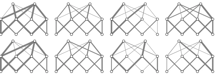
Figure 7: Two examples of final bias settings, in columns, for networks trained on the functions (left to right)f0,f1,f+,f× with different data orderings.
symmetry of this network, we only need to check four equivalence classes of functions. Here equivalence is with respect to negating inputs or the output, or swapping the two variables. In all cases, these operations on the function correspond to relabelings of the input and output nodes of the network. Using the algebra of GF(2) for Boolean operations, representatives of the four equivalence classes are
f0(z1, z2) = 0 f1(z1, z2) =z1 f+(z1, z2) =z1+z2 f×(z1, z2) =z1z2.
We have verified that the four functions above are learned on the 16-edge network with SDA and balanced weights (q= 1). The biases were always initialized at zero, as rendered by equal-thickness wires in Figure 6. Recall how the network is trained on a function f
with the SDA algorithm. After a data vector d= (z1, z2,z¯2,z¯1) is forward-propagated, the
two output nodes will have equal or unequal values. If unequal, and the correct node — corresponding to class f(z1, z2) — is smallest, no biases are changed and the next item
is processed. If the smallest output is positive but wrong, or equal to the other output, then the SDA algorithm executes iterations until the correct output is smallest or zero. The network will then have learned d, except for the case where the iterations drive both outputs to zero. This irreversible mode of classification ambiguity does not arise with the 16-edge network and any of the four functions.
In ultra-conservative learning there is no guarantee that successfully learned data is not unlearned in subsequent training. However, by testing on all four data each time biases are changed by SDA, one can establish whether the function is learned. The order in which data are processed matters, as manifested in the final bias values. Figure 7 shows two examples of final bias settings for each of the four functions.
changing and the data are correctly and unambiguously classified. Two numbers of interest in a successful trial are (i) #err, the total number of wrong or ambiguously classified data
(invocations of SDA) over the course of training, and (ii) #iter, the total number of SDA
iterations performed. These numbers are equal on the 16-edge network trained on any of the 2-variable functions, as one SDA iteration is sufficient to fix any incorrect classification in this case. Not surprisingly, the constant functionf0 is the easiest to learn, with #err= 1.
All trials with f1 have #err equal to 4 or 5. The xor function, f+, always has #err = 3,
while the and function,f×, has the greatest variation with #err= 2,3 or 4.
The more aggressive variant of SDA, where iterations continue until the class output node is zero, also succeeds for all four functions on the 16-edge network with balanced weights. In this mode of training one pass through the data always suffices. We find, for all four functions, that the network must see all the data (#err= 4) and 6≤#iter≤9.
Complete Boolean networks, such as the 16-edge network, quickly become too large for functions of many Boolean variables, and alternative network designs must be considered. For example, the nodes in the single hidden layer could be clauses formed from all small subsets of the variables, or even an incomplete sampling of such clauses. The success of clause learning (w → 0) with such networks would of course depend on the nature of the function.
The opposite limit applied to the hidden-layer weights, w → ∞, suggests a different design for single-hidden-layer networks. Because biases on edges to the outputs never change in this limit, we connect each hidden-layer node to a single output. The hidden-layer nodes are now interpreted as proto-clauses, because their composition in literals is modified during training by changes to the input biases. For example, a proto-clause could sample both a variable and its negation, and rely on training (bias change) to select one or the other. Moving bias changes to the input side of the network alleviates the exponential explosion of static clauses one faces in the w→0 limit.
The departure from complete Boolean networks we feel is most interesting is increasing the number of hidden node layers. Indeed, keeping training tractable in this setting was the primary motivation for the rectified wire model. To explore this feature we trained a network on three-variable Boolean functions where the hidden layer nodes only have in-degree two. To potentially express relationships among three variables, the hidden nodes are arranged in two layers.
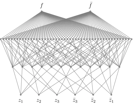
The three-variable network, shown in Figure 8, is complete in the following sense. The nodes in the first hidden layer exhaust the 3×4 ways of collecting inputs from distinct Boolean pairs, with and without negation. One attribute of these nodes is the identity of the Boolean variable — 1, 2 or 3 — that was not sampled. The second layer of hidden nodes exhausts all 3×4×4 combinations of input pairs for which this first hidden layer attribute is different. As in the 16-edge network, the wiring between the final hidden layer and the output nodes is complete in the conventional sense. The resulting network has 216 edges.
Bias renderings, after training, of networks with over 200 edges are not very comprehen-sible. However, the statistics of the numbers #err and #iter appear to correlate well with
Figure 8: A rectified wire network with two hidden layers that, we conjecture, learns all Boolean functionsf(z1, z2, z3) on three variables. All hidden nodes in this network
have two inputs.
to 0 and 1 with equal frequency:
f1(z1, z2, z3) =z1
f>(z1, z2, z3) =z1z2+z2z3+z3z1 f+(z1, z2, z3) =z1+z2+z3.
Learning f1, or learning to ignore z2 and z3, should be easiest. Function f>, the logical
majority function, we expect to be harder because its value, in some but not all cases, is sensitive to all three variables. By the same argument, the parity function f+ should be
the hardest of the three.
All trials we performed on f1, f> and f+, using SDA on the 216-edge network with
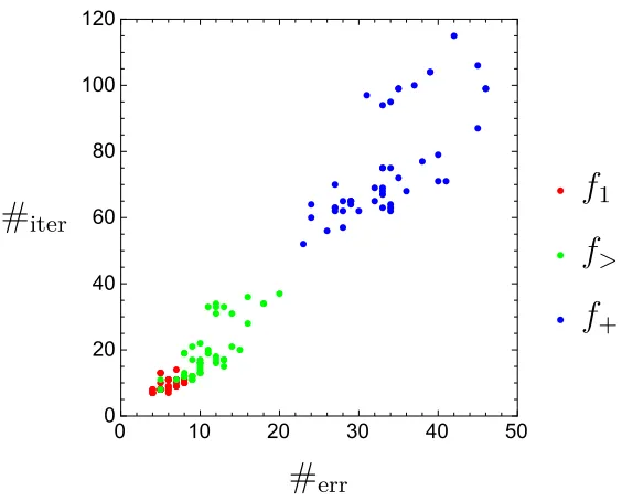
balanced weights, were successful. Figure 9 shows the distribution of #err and #iter in 50
trials for each, differing only in the order in which the data are processed. By either metric — the total number of false classifications or the total work in training — the difficulty ranking of the functions is f1 < f> < f+. Less extensive trials on the full set of 22
3
Boolean functions all proved successful and leads us to conjecture that the 216-edge network of Figure 8 learns all 3-variable Boolean functions regardless of data order.
We note that the complete Boolean network, with only 23(3 + 2) = 40 edges, would have
been much smaller in this instance and by theorem 5.3 can learn all the Boolean functions in thew→0 limit. Still, it is reassuring to see that SDA also works in deep networks.
zero-Figure 9: Distribution of #errand #iterin 50 trials when learning the three-variable Boolean
functionsf1,f> and f+ on the network shown in Figure 8.
output-value rule (xc= 0), we find that training is not always successful. While training on
f1 was always successful, the success rate onf> was 76% and onf+only 22%. The success
rate improves for smaller q and appears to be at 100% for all three functions whenq= 0.5. Another point in favor of ultra-conservative termination is the greatly reduced number of iterations. For example, by forcing zero outputs, the total number of iterations needed to learnf1, averaged over data ordering, is about 140, or about 15 times the number needed
by the ultra-conservative rule.
8. Sparse expander networks
A nice simplification provided by rectified wire networks is that the training algorithm has very few hyperparameters. Learning succeeds or fails mostly on the basis of the network we choose. However, it is possible that the tractability of rectified wire training comes at the cost of a greater sensitivity to network design. We therefore anticipate that network characteristics — size, depth, sparsity — will take over the role of hyperparameters.
As a general rule, learning improves with larger networks. Since the edge-biases are the only learned parameters of a rectified wire network, the appropriate measure of network size is the number of edges. In this section we introduce a family of networks that adds depth — the number of hidden layers — as a second design parameter.
extends, during training, to the bias updates on all edges between the hidden nodes. To allow for independent settings of the biases, the initial biases must break the symmetry in some data-neutral fashion. Incompletely connected or even sparse networks are an extreme form of symmetry breaking, and correspond to infinite bias settings.
Our network design, calledsparse expander networks, generalizes the networks of section 7. Sparsity in our case is the property that all the hidden nodes have in-degree of only two. At the same time, the representation of the data is expanded, layer to layer, by a constant growth factorg in the size of layers. The expander structure cannot be applied to the final two layers because of the fixed (and small) number of output nodes. Here the layers are completely connected, thereby making all the information in the last (largest) hidden layer available to each output node. Lettinghdenote the number of hidden layers, the number of edges in a sparse expander network for|D|inputs and |C| classes, with parameters (g, h), is
|E|=|D|(2g+· · ·+ 2gh−1+ (2 +|C|)gh). (17)
To introduce a degree of uniformity, our networks have a constant out-degree of 2g on all input and hidden nodes. This requires that g is an integer. The in-edges to the nodes in a hidden layer are generated by the simplest random algorithm. In a first pass through the hidden layer we create one edge per node to the layer below by drawing uniformly from the nodes that currently have the smaller of two possible out-degrees. A second edge is added in a second pass, at the completion of which all the nodes on the layer below will have out-degree 2g. Edges from the first hidden layer to the input layer are constructed no differently. This construction is implemented by the publicly available1C programexpander
and was used for all the experiments reported in the next section.
We can use the hyperparameter q to assess the role of depth. If performance does not degrade in the limitq→0, then the network could have been replaced by the much simpler single-hidden-layer model (16). When this limit is applied to a sparse expander network, the number of hidden nodes is |H|= |D|gh. The sampling of the fixed weights aji in the
rectifier gates is also controlled by g and h.
9. Experiments
To describe experiments with conservatively trained rectified wire networks it suffices to specify the network. The SDA algorithm has no other hyperparameters, since there even is a balancing principle that sets the weights. The two-parameter sparse expander networks offer a convenient way to study behavior both with respect to network size and depth. These characteristics were our main focus and guided the choice of experiments going into this study. Follow-up experiments, that featured the weight-multiplier hyperparameter q, later provided critical insights for network design that have yet to be explored.
All our experiments were carried out with a publicly available1 C implementation of the SDA algorithm called rainman. This program requires that the user-supplied network is layered and the number of inputs and outputs are compatible with the data. Our networks were all created by the programexpander.
Although rainman reports results at regular intervals, after a specified number of data have been processed, this “batch size” has no bearing on the actual training because bias parameters are only updated in response to wrong classifications. The batch size merely sets the frequency with which the network is tested against a body of test-data. The main result of this test is the classification accuracy: the test-data average of the indicator variable that is 1 for correct, unambiguous classifications, and 1/mwhen the correct class node is in an
m-fold tie.
In addition to the classification accuracy,rainmanalso reports a number of other quan-tities of interest. Two we have already seen in section 7: the running total of misclassi-fications, #err, and the work (iterations) performed so far by SDA, #iter. These should
increase while the classification accuracy is below 100%. However, in an “overfitting” sit-uation #err and #iter stop increasing before the accuracy has reached 100%. Evidence of
this phenomenon is more directly discerned through another statistic reported byrainman: the average number of SDA iterations required to fix each of the incorrect classifications encountered in the batch, h#iteri. As defined, h#iteri is never less than 1. However, when
there are no misclassifications in the batch at all (keeping #err and #iter static), the value h#iteri= 0 is reported.
Information more revealing of the internal workings of the network is provided by the layer-averages of the edge activations,hα1i, . . . ,hαhi. Here hαhi is the fraction of edges, in
the layer leading to the output nodes, that are active in an average test-data item. These numbers decrease during training, a result of biases being increased.
Lastly, a statistic relevant to the termination of training is the frequency, in the test-data, of irreversible misclassifications, h0erri. The latter arise whenever an output node,
not of the correct class, has value zero. The onset of h0erri > 0 signals that training
should terminate because activation levels are so low that SDA is forced to make multiple outputs zero even while targeting just the class output. A simple remedy for preventing
h0erri>0 is to increase the size of the network. The case ofm-fold classification ambiguities,
mentioned above, occurs in practice only whenmoutput nodes are tied at zero. Ambiguous classification is therefore not a problem as long as h0erri>0.
On a single Intel Xeon 2.00GHz core rainman runs at a rate of 50ns per iteration per network edge. Multiplying this number by the product of #iter and |E| (17) gives a good
estimate of the wall-clock time in all our experiments.
9.1. Nested majority functions
We first describe experiments with a synthetic data set. Synthetic data has some advantages over natural data. Our nested majority functions (NMF) data has two nice features. First, through the level of nesting we can systematically control the complexity of the data. Second, because these Boolean functions are defined for all possible Boolean arguments, it is easy to generate large training sets for supervised learning.
NMFs are a parameterized family of Boolean functions that evaluate to 0 and 1 with equal frequency. The first parameter, a prime p, sets the number of arguments at p−1. Instances are defined by three integers a, b, c ∈ {1, . . . , p−1} and a nesting level n = 0,1,2, . . . . Starting with
Figure 10: An instance of a depth 5 nested majority function on 6 variables. The nodes are majority gates and the two edge colors indicate the presence/absence of negation. The depth 4, . . . ,1 functions correspond to removing 1, . . . ,4 layers from the bottom of the circuit.
the other functions (taking values in GF(2)) are defined via the recurrence
fan=f>
f(nab−1mod p)+z(ac), f(2n−1ab mod p)+z(2ac), f(3n−1ab mod p)+z(3ac)
,
wheref> is the 3-argument majority function and
z(x) = (xmod p) mod 2
should be interpreted as an element of GF(2). The functions fn at level n correspond to depth-n Boolean circuits taking p−1 inputs and constructed from not and majority gates. Figure 10 shows an instance of the functionf5 forp= 7.
From the identity
f>(z1+ 1, z2+ 1, z3+ 1) =f>(z1, z2, z3) + 1
it follows that negating all the arguments of a NMF negates its value. The two classes, defined by the NMF value, are therefore equal in size.
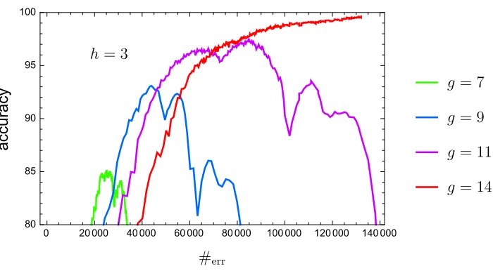
Figure 11: Improvement of the classification accuracy with network size, for the function
f13, on rectified wire networks with three hidden layers.
more arguments and with more complicated rules. The possibility of generalizing the value of fn, from many fewer than 2p−1 data, is clearly only possible for smalln. Our results go
as far asn= 4.
We generated training and test data samples (of the 30 Boolean variables) with a pseudo-random number generator. In the longest experiment, with 107 training samples, less than 1% of the data was seen more than once by the training algorithm.
We first present results for the functionf13. Fixing the number of hidden layers ath= 3, Figure 11 shows the effect of increasing the network size via the growth factor g. The accuracy is plotted as a function of #err, rather than the number of training data, because
learning (change of bias) occurs only when there has been a misclassification. In all except the g = 14 network (683760 edges), the accuracy reaches a maximum after which there is a sharp decline that coincides with the onset of h0erri > 0. The smaller networks could
still serve as imperfect classifiers by terminating their training at the empirical maximum test accuracy, or, in the absence of test data, when h0erri exceeds a threshold. We have
no explanation of the intriguing similarity of the unsuccessful accuracy plots. We also find that many of the seemingly random features in the accuracy plots are nearly reproduced in different random instances of expander networks with the same (h, g).
We emphasize that it is not really surprising that generalization performance can dras-tically deteriorate with more training examples for small networks. Conservative learning is using a fundamentally different principle than the standard approach that tries to min-imize an overall loss function across training examples. Conservative learning is merely trying to myopically account for the most recently seen example, which can have negative consequences for other training examples, to say nothing of unseen test examples.