R E S E A R C H A R T I C L E
Open Access
Matching methods to create paired survival
data based on an exposure occurring over
time: a simulation study with application to
breast cancer
Alexia Savignoni
1,2,3*, Caroline Giard
1,4, Pascale Tubert-Bitter
2,3and Yann De Rycke
5Abstract
Background: Paired survival data are often used in clinical research to assess the prognostic effect of an exposure. Matching generates correlated censored data expecting that the paired subjects just differ from the exposure. Creating pairs when the exposure is an event occurring over time could be tricky. We applied a commonly used method, Method 1, which creates pairsa posterioriand propose an alternative method, Method 2, which creates pairs in “real-time”. We used two semi-parametric models devoted to correlated censored data to estimate the average effect of the exposureHR(t): the Holt and Prentice (HP), and the Lee Wei and Amato (LWA) models. Contrary to the
HP, theLWAallowed adjustment for the matching covariates (LWAa) and for an interaction (LWAi) between exposure
and covariates (assimilated to prognostic profiles). The aim of our study was to compare the performances of each model according to the two matching methods.
Methods: Extensive simulations were conducted. We simulated cohort data sets on which we applied the two matching methods, theHPand theLWA. We used our conclusions to assess the prognostic effect of subsequent pregnancy after treatment for breast cancer in a female cohort treated and followed up in eight french hospitals. Results: In terms of bias andRMSE, Method 2 performed better than Method 1 in designing the pairs, andLWAawas
the best model for all the situations except when there was an interaction between exposure and covariates, for whichLWAiwas more appropriate. On our real data set, we found opposite effects of pregnancy according to the six
prognostic profiles, but none were statistically significant. We probably lacked statistical power or reached the limits of our approach. The pairs’ censoring options chosen for combination Method 2 -LWAhad to be compared with others. Conclusions: Correlated censored data designing by Method 2 seemed to be the most pertinent method to create pairs, when the criterion, which characterized the pair, was an exposure occurring over time. In such a setting, the
LWAwas the most appropriate model.
Keywords: Matching on time-dependent covariates, Matched time-to-event data, Correlated survival data, Event occurring over time, Stratified Cox model, Marginal Cox model, Pregnancy, Breast cancer, Simulation study
*Correspondence: [email protected]
1Service de Biostatistique, Institut Curie, 26 rue d’Ulm, 75005 Paris, France 2Inserm, CESP Centre for research in Epidemiology and Population Health, U1018, Biostatistics Team, F-94807 Villejuif, France
Full list of author information is available at the end of the article
Background
Five percents of breast cancers occur among women before the age of 40 and in fewer than 2% of women under 35 [1]. Physicians are more and more faced with issues of post-treatment pregnancy, such as the optimal time before considering conception. In physiopathologi-cal terms, a pregnancy after breast cancer is not advisable, especially in patients with positive hormonal receptors [2,3]. However, many observational studies report that pregnancy does not have any impact on the evolution of breast cancer [4-6], and could even have a long-term pro-tective effect [2,6-10]. This phenomenon can be due to the so-called “healthy mother bias” [7],i.e. only women who are in good health will undertake a pregnancy after treatment for breast cancer.
Pregnancy is therefore related to the prognostic con-dition of the patient, and its occurrence might change the prognostic effect of some factors, for instance, the hormonal receptors. The prognosis of positive hormonal receptors could be qualitatively (interaction) different before and after pregnancy (i.e.interaction between hor-monal receptor and pregnancy).
In an attempt to control for this “healthy mother effect”, various statistical approaches have been used. Some authors used the standard Cox model [11] with preg-nancy considered as a covariate whose value depends on time, and adjusting for the known prognostic factors at the diagnosis of cancer, reflecting the gravity of the dis-ease [2,6,8,9]. In spite of this adjustment for disdis-ease grade at diagnosis, pregnancy still remained a significant good prognostic factor, indicating a long-term protective effect of pregnancy, which is difficult to explain and to interpret. Others tackled the problem from the angle of an “illness-death” model [12-14] which makes it possible to describe the natural history of the disease, taking into account the prognostic profiles of the patients who had or did not have a pregnancy [15]. This model provided better under-standing and interpretation of the effect of pregnancy by comparing transition probabilities to relapse between women who had or did not have a pregnancy. Moreover, taking into account a possible interaction between prog-nostic profiles and the pregnancy improved the estimation of the pregnancy prognostic effect. Overall prognosis was not adversely affected by subsequent pregnancy. How-ever, to allow adjustment, such a complex model requires enough pregnancies and events of interest.
In both previous approaches, the adjustment relied only on known prognostic factors. However, measured prog-nostic factors might not be enough to characterize the prognostic status in such a disease. Matching subjects designs might be helpful to accomplish that.
Other researchers have conducted paired studies: preg-nant and non-pregpreg-nant women were matched on the main known prognostic factors (hormonal receptor,
proliferation level, nodal involvement, use of chemother-apy, year of diagnosis), and the non-pregnant had to be disease-free for as long as the time from diagnosis to preg-nancy of the pregnant women [3-5,7,10]. By this matching carried out on known and measured factors, one can suppose that the subjects of the same pair also share non-observable, not observed or not measured factors, in addition to the factors of pairing. Thus, this design may improve the control of the “healthy mother effect” compared to the two approaches presented above.
However, to our knowledge, in such a case and con-trary to the first methods cited previously, researchers [3-5,7,10] did not take into account the fact that preg-nancy was an event occurring over time. They matched the pregnant woman to a non-pregnant one a posteri-ori,i.e.at the end of the follow up study, knowing which women were pregnant and which were not over the study period. They analyzed the data as if these pairs were a priori known and created at diagnosis, i.e. at time t = 0. Moreover, they always used the stratified Holt and Prentice semi-parametric model (HP) [16] to estimate the pregnancy prognostic effect, whereas other semi-parametric models devoted to censored correlated data are available such as frailty models [17,18] and marginal models [19-22]. Frailty models model the time distribu-tion condidistribu-tionally to a random effect (frailty covariate), specific to each pair, and which is not observed. The struc-ture of correlation has to be defined. The latter leave the nature of dependence among paired failure times com-pletely unspecified.
Non-parametric [23,24] and parametric [25] approaches have been developed, but we focus on the semi-parametric approach, more specifically on the commonly used marginal semi-parametric model. This marginal approach was developed by Wei, Lin and Weissfeld [19] to analyze subjects with multiple events, and then Lee, Wei and Amato [20] adapted it to clustered subjects.
In this paper, we use the marginal paired proportional hazards model of Lee, Wei and Amato (LWA) [20] and the Holt and Prentice stratified model [16] (HP). The main difference between them lies in the ability of theLWA[20] model to adjust for matching covariates and for the pos-sible interaction between the covariate and the exposure, contrary to theHPmodel. Mehrotraet al.[26] proposed an efficient alternative to the stratified Cox model analysis to estimate the exposure effect, which does not require the assumption of a common hazard ratio across strata. How-ever, that model is not adapted to our particular context of a large number of strata, with very small sample size per stratum (in our work, a stratum is a pair), thus it will not be studied here.
designing the pairs “in real-time” by taking into account the occurrence of the event over time, i.e. the preg-nancy, which characterizes the subject’s group within the pair.
The goal was to determine the combination between matching methods (a posterioriand in “real-time”) and models (HPandLWA), which is the most efficient in terms of bias and Root Mean Square Error (RMSE) to estimate and test the pregnancy prognostic effect. In the follow-ing, pregnancy is referred to as the “exposure” occurring over time and the pairs are composed of an exposed and a non-exposed subject.
In the next section, the two matching methods as well as the models of analysis are presented. In Section ‘Simulations’, extensive simulations are used to analyze the performance of these Method - Model combina-tions in term of bias and RMSE of the estimated effect related to the exposure occurring over time. In Section ‘Real data application’, our findings are applied to real data in order to analyze the effect of a subsequent preg-nancy on breast cancer evolution [9]. A brief discussion concludes the paper.
Methods
The subjects are matched on all the known prognostic factors represented by vectorZ. In the following, indexj corresponds to the rank of the exposed subject occurring at thejth position’s order among theneexposed subjects at the end of the study (j= 1,. . .,ne), and indexi corre-sponds to the subject among thensubjects of the study (i=1,. . .,n). Lettibeing defined as the follow-up time of each subjecti, andtEias the time exposure for a subjecti; for a subject who is never exposed, we considertEi= +∞. Rm(t) represents the subjects at risk of event and non-exposed at timetfor the methodm(m=1 or 2). Let the set of paired subjects being defined asPj = {j,i(j)}, with i(j) the subjecti of RmtEj
chosen for thejth exposed subject.
The two matching methods
The two matching methods applied in the context where exposure is an event occurring over time, are presented.
Method 1 matches the subjects as follows: all the sub-jectsi exposed (tEi < +∞) are matched with a subject who was not exposed during the whole period of follow-up. This method is called ana posteriorimethod because the groups exposed and non-exposed are defined at the end of the study and are considered to be known and created at time t = 0. According to Method 1, if a subject j undergoes an exposure at time tEj, then the eligible subject’s set R1
tEj
of subjects i eligible to be matched to j could be written as follows: R1tEj
=
i=j/ti≥tEjANDtEi= +∞. This approach has been
commonly used in the literature [3-5,7,10] with exposure not being considered as time-dependent.
As exposure is a time-dependent event, a second approach is proposed which designs the pairs “in real-time”: according to Method 2, if a subjectjundergoes an exposure at timetEj, then the eligible subject’s setR2
tEj
of subjectsieligible to be matched tojat timetEj, could be written as follows: R2
tEj
= {i = j/ti ≥ tEj AND tEi > tEj}. R2
tEj
includes subjects at risk that are not yet exposed attEjand will be exposed after, and subjects who will never be exposed. A pair composed of an exposed subject and a non-exposed one who would never undergo the exposure is called a “perfect pair”, whereas it would be an “imperfect pair”. As a result, the non-exposed subject of an imperfect pair could be matched after exposure with another non-exposed subject.
Method 2 is similar to the one proposed by Lu et al. in case-cohort studies [22] where the membership in the exposed and unexposed groups is the outcome to be explained, whereas in our work it is an explanatory variable.
For both methods, exposed and not exposed subjects are matched according to the covariate vectorZ, and the not exposed subject has to be disease-free for as long as the time from the starting point (disease diagnosis) to the exposure time.
For both methods, if several non-exposed subjects can be matched with an exposed one, the matched non-exposed subject is randomly chosen from the set of eligible subjects Rm(t); if no non-exposed subjects are available, the exposed subject cannot be paired and is thus excluded from the analysis.
Note that even if a subject could belong to two differ-ent pairs with Method 2, these two pairs are independdiffer-ent while they are never at risk at the same timet.
The statistical models
In the following,λi(t)is the instantaneous hazard function of outcome to be estimated for pairPj. It is notedλi(t,Zi) to specify that the estimation is made on the pairPj, which is composed of the exposed subjectjand the non-exposed subjectimatching onZi. This notation is the same for all the models studied, even those where the adjustment for Ziis not available.
For all the models presented below,Ei(t)corresponds to the time-dependent exposure status and is defined as follows:Ei(t) = 0 ift < tEi, and Ei(t) = 1 ift ≥ tEi. The pair of subjects is also defined by a time-dependent covariate:Pi(t) = jifi∈ Pjandt∈[tEj;ti] , orPi(t) =0 otherwise.
Holt and Prentice stratified Cox model
The instantaneous hazard function is written for each subjectias
λi(t,Zi)=λ0i(j)(t)exp(γ (t)Ei(t)) (HP)
λ0i(j)(t)is a pair-specific baseline hazard function that is assumed to be identical for both subjects of pairPj, con-sidered here as strata; it is concon-sidered as a nuisance param-eter not to be estimated. The exposure effect exp(γ (t)) is then estimated, considering the between-pair hetero-geneity, by allowing the instantaneous baseline hazard to be different within each pair. It is assumed to be iden-tical across strata (no interaction between the exposure and the pairs) and thus to be implicitly common for the whole exposed population: exp(γ (t)) is defined as the population-weighted average of the stratum-specific haz-ard ratios. However, if this assumption is incorrect, i.e. in the presence of a true (and often undetected) interac-tion, using this model leads possibly to a biased and/or less powerful analysis [26].
Furthermore, with this model, estimation of the expo-sure effect cannot be adjusted for a possible interaction between the matching factors and the exposure. This stratified approach is sensitive to the unit number per strata and to the number of strata: the accuracy of the regression coefficients decreases for a small number of units per strata and/or many numbers of strata [27].
This model is implemented in R software [28] through the coxphfunction by including the term “strata(Pi(t))” with the other explanatory covariates.
Lee, Wei and Amato Cox model
The marginal LWA model [20] is an alternative to the standard Cox model [11] and is written as follows
λi(t,Zi)=λ0(t)exp(γ (t)Ei(t)), (LWAu) if the exposure effect is not adjusted for the matching covariates vectorZ;
λi(t,Zi)=λ0(t)exp
βZi+γ (t)Ei(t)
, (LWAa)
if the exposure effect is adjusted for the matching covari-ates vectorZ;
λi(t,Zi)=λ0(t)exp
βZ
i+γ (t)Ei(t)+α(t)ZiEi(t)
, (LWAi)
if the exposure effect is adjusted for the matching covari-ates vectorZ, and for the interaction betweenZand the exposure.
For each of these threeLWAmodels,λ0(t)is an unspec-ified marginal baseline hazard function considered as common for all the pairs, so for the whole population. As above, it is considered as a nuisance parameter; exp(γ (t)) is the average time-varying exposure effect as in theHP model, but adjusted (LWAa) or not (LWAu) for covariates Zand for the possible interaction between covariates and
exposure (LWAi). Like the standard Cox model [11], the LWAassumes that all sample subjects are homogeneous (all subjects have the same λ0(t)) in spite of the possi-ble adjustment for covariates (unique difference between LWAuandHP).
This model is implemented in R software through the coxphfunction, by including the term “cluster(Pi(t))” with the other explanatory covariates.
For both models, the Proportional Hazard Assumption (PHA) was evaluated by Harrel’s test on scaled Schoënfeld residues. This test is implemented in R software through thecox.zphfunction. The possible time-dependent effect of the exposure was taken into account by time intervals chosena posteriori, and not by a time-specified function.
Note that the combination HP and Method 1, taking the exposure as a time-dependent covariate or not, gave exactly the same estimation ofHR(t), whereas LWAdid not.
Table 1 presents all the models according to the adjust-ment or not for covariates.
In the following, different simulations and analyses were performed with R software version 2.13.0.
Results Simulations Objective
The main objective of the simulation study was to assess the ability of the HP and LWA models to estimate the true effect of exposureHR(t), defined by exp(γ (t)), in a context of matched paired survival data, where the pairs were designed according to the two different methods described previously. The aim was to establish the most efficient Method - Model combination.
Dataset
Simulation of cohort data - Procedures and scenar-ios chosen. All the details of the cohort data simulation and the procedures and scenarios chosen are given in Appendix A.
We simulated the cohort data referring to an “illness-death” model with transition intensitiesλ12(t),λ13(t)and λ23(t)(Figure 1). The parameter of interestHR(t) corre-sponded to the ratioλ23(t) /λ13(t). The averageHR(t)is obtained from an exact formula involving the averages of λ13(t)andλ23(t)which are computed through a numer-ical approximation (transformation of the time from con-tinuous to discrete values) (See the Appendix B). The average HR(t) adjusted for the different covariates was estimated empirically: its estimation was obtained using large size samples to guarantee good precision. Moreover, note that the larger the ratioλ12(t) /λ13(t), the larger the number of exposures in the simulated cohort.
Table 1λi(t, Zi)estimations with theHPandLWAmodels are associated to theHR(t)to be estimated according to the
adjustment for covariates
Exposure covariate Models HR(t)
HP LWA
λi(t,Zi) λi(t,Zi)
Time-dependent
and no time-dependent effect λ0i(j)(t)exp(γEi(t)) λ0(t)exp(γEi(t)) HR(t)
With adjustment forZ λ0(t)exp
γEi(t)+βZi
HRa(t)
and with interaction λ0(t)expγEi(t)+βZi+α(t)ZiEi(t) HRi(t) Time-dependent
and time-dependent effect λ0i(j)(t)exp(γ (t)Ei(t)) λ0(t)exp(γ (t)Ei(t)) HR(t)
With adjustment forZ λ0(t)expγ (t)Ei(t)+βZi HRa(t)
and with interaction λ0(t)expγ (t)Ei(t)+βZi+α(t)ZiEi(t) HRi(t)
λi(t,Zi)is the instantaneous risk function of event for the pairPj, which is composed of the exposed subjectjand the non-exposed subjectimatching onZi.
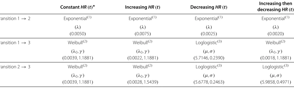
covariatesZk (k = 1, 2 or 3). At timet = 0, there were 23=8 possible profiles ofZfactors.
The simulation model included (i) the choice of an instantaneous baseline risk function λuv(t,Z) for each of the three transitions u → v (Table 2), (ii) the choice of theZeffects, exp(βuvk), for each transition,i.e.
λuv(t,Z) = λ0,uv(t)exp(βuv1Z1+βuv2Z2+βuv3Z3)and (iii) the choice for the censoring proportion.
For (i), an instantaneous average risk function λuv
t,Z=Zfor each of the three transitions was sim-ulated. Table 2 displays the λuv
t,Z=Z distributions of each transition used for each of the five different configurations ofHR(t).
For (ii), ten differentβuvk scenarios considered as plau-sibleβuvkclinical values [9,15], were performed. Given the five configurations chosen for HR(t) and these ten βuvk scenarios, 50 different situations were obtained.
Finally, for (iii), these previous 50 situations were first performed without censoring. Two levels of inde-pendent uniform censoring were implemented only to
the following βuvk scenario: β
12 = (−0.2,−0.4,−0.8), β13 = −β12 andβ23 = β12; and they were applied to each of the five configurations ofHR(t). This yielded to 10 more situations.
For each of the 60 situations, 1000 different data sets were generated with a sample size of 2000 subjects. At t = 0, these 2000 subjects were allocated to eightZ pro-files. Att > 0, the 250 subjects of the 8 different profiles will be divided up in the three transitions and will change over time according to the fiveHR(t)configurations.
All theoretical values ofHR(t)were calculated on the simulated cohort data. They were computed in the over-all correlated censored data and inside each sample of the Zprofile. The averageHR(t)was calculated without and with adjustment for the matching covariates,i.e. HR(t) andHRa(t) respectively.HRi(t) is the one estimated in eachZprofile.
From the correlated censored data,HPandLWAu mod-els are both assumed to give an averageHR(t)i.e. HR(t) (considering different assumptions), so they are the only
State 1
Breast cancer
diagnosis
State 2
Pregnancy
State 3
Outcome
λ
13(t)
Table 2 Survival functions applied to simulate each transition and each selected configuration
ConstantHR(t)∗ IncreasingHR(t) DecreasingHR(t) decreasingIncreasing thenHR(t)
Transition 1→2 Exponential(1) Exponential(1) Exponential(1) Exponential(1)
(λ) (λ) (λ) (λ)
(0.0050) (0.0075) (0.0025) (0.0020)
Transition 1→3 Weibull(2) Weibull(2) Loglogistic(3) Weibull(2)
(λ0,γ ) (λ0,γ ) (μ,σ ) (λ0,γ )
(0.0039, 1.1881) (0.0022, 1.1881) (5.7146, 0.2390) (0.0018, 1.1881)
Transition 2→3 Weibull(2) Weibull(2) Loglogistic(3) Loglogistic(3)
(λ0,γ ) (λ0,γ ) (μ,σ ) (μ,σ )
(0.0039, 1.1881) (0.0028, 1.5439) (5.6778, 0.2463) (5.9858, 0.4971)
(1)S(t)=exp(−λt);(2)S(t)=exp(−(λ0t)γ);(3)S(t)=[ 1+exp(ln(t)−μ σ )]−1.
*We simulated the same functions and parameters for the second ConstantHR(t)except for Transition2→3whereλ
0=0.0069.
two models which could be compared. Fitting of model LWAamakes it possible to estimate an averageHR(t)i.e. HRa(t), whileLWAiis assumed to giveHRi(t)for each Z profile (Table 1).
As the exposure effect was considered to change over time for three of the five configurations, its estimation was assessed by time interval specifieda posteriori.
Matching methods - Creation of censored correlated data from cohort data. For each data set, the two match-ing methods presented in Section ‘Methods’ were applied. According to Methods 1 and 2, the two subjects in each pair were matched on the three covariates Zk, and the non-exposed subject had to be disease-free for as long as the time from t = 0 to exposure time of the exposed subject.
Then from the 2000 subjects simulated in cohort data sets and equally allocated to the 8Zprofiles, a number of pairs smaller or equal to the number of subjects in State 2 (i.e.pregnancy) were obtained. This latter depended on the situation simulated, resulting from theHR(t) config-uration, theβuvkscenario and the censoring percent.
Statistical criteria used to compare the perfor-mances of the different estimators. To estimate a time-dependent effect, the time interval [0−tmax] was divided intoLtime intervalsIl defineda priori, according to the HR(t)configuration, and written as follows:
a0=0<a1< . . . <aL=tmax
and
Il =[al−1;al[,l≥1.
If there was no interaction and no time-dependent effect, an estimation γˆs was obtained that corresponded to the estimation ofγ performed in thesthsimulation set inside the sameHR(t)configuration.
If there was an interaction and no time-dependent effect, an estimation for each of the 8Zprognostic profiles was obtained and expressed asγˆs+αˆ
sZ.
If there was no interaction and a time-dependent effect, an estimation for each of theIltime intervals was obtained and expressed asγˆsl.
If there was an interaction and a time-dependent effect, 8×Lestimations were obtained and expressed asγˆsl +
ˆ
αslZ.
To assess the combination Method - Model to estimate HR(t), the bias and the RMSE of the estimations pre-sented above were calculated. The 8Zprofiles are indexed byw=1 to 8, and the profile w is notedZ(w).
In the event of with an interaction and a time-dependent effect, the bias was estimated for eachland eachZ(w)over the 1000 simulations as follows:
blZ(w)= 1 1000
1000
s=1
ˆ
γsl+αˆ slZ−
γl+α
lZ
=γl+αlZ−
γl+α
lZ
and
RMSElZ(w) = b2lZ(w)+V
ˆ
γl+αˆ lZ
,
where, in each Il interval, γl+αlZ is the mean and
V
ˆ
γl+αˆ lZ
the empirical variance of the 1000
parame-ters estimatedγˆsl+αˆ slZ:
V
ˆ
γl+αˆ lZ
= 1
(1000−1) ⎡ ⎢
⎣1000s=1 γˆsl+αˆ slZ
2
−
1000 s=1
ˆ
γsl+αˆ slZ
2
1000
To compare the different combinations Method -Model, the bias was averaged over the profiles (bl•)or over the time intervals(b•Z(w))or both(b••).
b•Z(w) = 1 L
L
l=1 blZ(w)
bl• = 1 8
8
w=1 blZ(w)
b•• = 1
8 8
w=1 b•Z(w)
The associatedRMSEs are given by
RMSE•Z(w) =
1
L L
l=1
b2lZ(w)+V
ˆ
γl+αˆ lZ
RMSEl• =
1
8 8
w=1 b2
lZ(w)+V
ˆ
γl+αˆ lZ
RMSE•• =
1
8 8
w=1 1 L
L
l=1 b2
lZ(w)+V
ˆ
γl+αˆ lZ
Note that if the exposure effect is not time-dependent, thenL=1. If there is no interaction between the exposure and the prognostic profiles, thenα=0.
Results
One particular situation among the 60 simulated is described. Figure 2 displays the increasing then decreas-ingHR(t)configuration, for each profile and on average, without censoring and with β12 = (−0.2,−0.4,−0.8), β13 = −β12 and β23 = −β13. In this particular sit-uation which corresponds to a “healthy effect” because of the negative values of β12, Figure 2 shows three different overall effects of the exposure: a pejorative one in the three better prognostic profiles (PP) (Z ∈ {(0, 0, 0),(0, 0, 1),(0, 1, 0)}), no effect in the intermediate PP (Z ∈ {(0, 1, 1)}) and a protective effect in the last four PP (Z ∈ {(1, 0, 0),(1, 0, 1),(1, 1, 0),(1, 1, 1)}). With β23 = −β13, we force an interaction betweenZand the exposure. Note that in this particular configuration cho-sen, whereβ23= −β13,HR(t)HRa(t)and their values are so close that the difference between them is not visible in Figure 2.
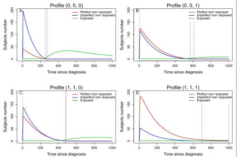
Number of pairs. Inside each profile, the maximum number of pairs was determined by the number of exposed subjects. With Method 1, this number was also limited by the number of “perfect” non-exposed subjects, but not with Method 2 since the non-exposed subject set
was composed of “perfect” and “imperfect” non-exposed subjects. The difference between the number of pairs from the two methods depended on the number of expo-sures: the larger the number, the larger the difference. We computed the relative difference (RD) in number of pairs between the two methods defined as
RD=Number of pairs with Method 2−Number of pairs with Method 1
Number of pairs with Method 1 ,
whose median was equal to +55% (range, +23% to +220%). Figure 3 represents the distribution of the number of pairs according to the profiles and to the matching methods: the median number with Method 2 was always larger than or equal to that with Method 1.
Figure 2HR(t)configuration chosen.Increasing then decreasingHR(t)configuration, for eachZprofile and on average, without censoring and withβ12=(−0.2,−0.4,−0.8),β13= −β12andβ23= −β13. This figure displays the theoretical estimations ofHR(t)called “mean”,HRa(t)called “adjusted mean” andHRi(t)in the eight prognostic profiles. The profileZ=(0, 0, 0)at timet=0 is the profile with the better prognosis; the profile Z=(1, 1, 1)has the worse prognosis, and the 6 others an intermediate prognosis. In this particular configuration chosen, whereβ23= −β13, HR(t)HRa(t)and their values are so close that the difference between them is not visible in this figure.
50
100
150
Profiles
Number of pairs
Numbers of pairs
according to the profiles and the pairs design's methods
(0, 0, 0) (0, 0, 1) (0, 1, 0) (0, 1, 1) (1, 0, 0) (1, 0, 1) (1, 1, 0) (1, 1, 1)
M1
M2
Figure 3Number of pairs.Distribution of the number of pairs according to the profiles and to the matching methodsM1andM2. Results obtained
0 200 400 600 800 1000
0
5
0
100
150
200
Time since diagnosis
Subjects n
umber
Profile (0, 0, 0)
Perfect non−exposed Imperfect non−exposed Exposed
A
0 200 400 600 800 1000
0
50
100
150
200
Time since diagnosis
Subjects n
umber
Profile (0, 0, 1)
Perfect non−exposed Imperfect non−exposed Exposed
B
0 200 400 600 800 1000
0
5
0
100
150
200
Time since diagnosis
Subjects n
umber
Profile (1, 1, 0)
Perfect non−exposed Imperfect non−exposed Exposed
C
0 200 400 600 800 1000
05
0
100
150
200
Time since diagnosis
Subjects n
umber
Profile (1, 1, 1)
Perfect non−exposed Imperfect non−exposed Exposed
D
Figure 4Number of subjects in the three possible groups.Number of subjects pertaining to the three possible subjects groups at each timet: the exposed subject (solid green line), the non-exposed subject who never will undergo the exposure (solid red line) and the non-exposed subject who will undergo the exposure (solid blue line). The dotted vertical green line represents the time of first exposure,i.e.the time of occurrence of the first pair; the dotted vertical blue line corresponds the time of the last perfect pair’s creation; and the dotted vertical red line corresponds the time of the last imperfect pair’s creation. Results obtained with the increasing then decreasingHR(t)configuration, without censoring and with
β12=(−0.2,−0.4,−0.8),β13= −β12andβ23= −β13.
larger depending on the censoring percent: the higher the censoring percent, the smaller the RD.
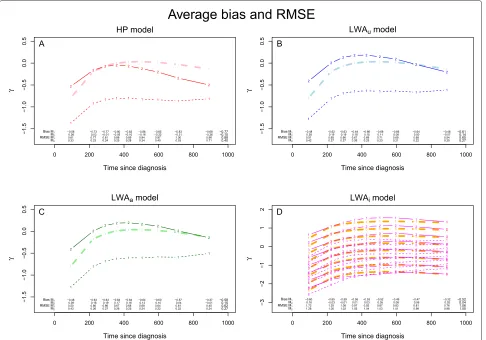
Bias and RMSE. Figures 5 displays the distribution of the bias and theRMSE of the exposure effect estimator, according to our four models.
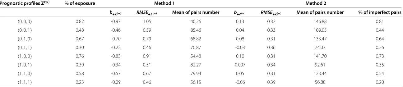
With Method 1, the estimation of HR(t) was biased with HP andLWAu, but more with HP; the estimation of HRa(t) was biased withLWAa. Whatever the model applied, HR(t) (HP, LWAu) and HRa(t) (LWAa) were underestimated, i.e. a poor prognostic exposure effect tended to be ignored and a no exposure effect tended to become a protective one. In eachZprofile,LWAi always largely underestimatedHRi(t)(Figures 5). The biasb••is equal to−0.77,−0.61,−0.58 and−0.52 underHP,LWAu, LWAaandLWAimodels, respectively; and theRMSE••is equal to 0.88, 0.65, 0.62 and 1.06 underHP,LWAu,LWAa andLWAi models, respectively (Figures 5). The bias and RMSEare given by PP in Table 3.
With Method 2 where HR(t) HRa(t), LWAu and LWAagave very similar values, whereasHPgave a smaller estimation ofHR(t) thanLWAu. All these three models are very close to the true value of the effect of exposure, but none gave an unbiased estimation: this estimation was slightly over- or under-estimated according to the time, but much less than with Method 1.HRi(t) was overesti-mated in some Zprofiles: HRi(t) was overestimated in the three PP,Z ∈ {(0, 0, 0),(1, 0, 0),(0, 1, 0)}, where the ratioλ12(t)
λ13(t) was large and then the proportion of imperfect pairs in the set of pairs to be analyzed, was also large (Figures 5). The mean of the time-dependent biasb••
al.
BMC
Medical
Research
Methodology
2014,
14
:83
Page
10
of
18
Table 3 Simulations results: time-dependent biasb•Z(w)withRMSE•Z(w)for theLWAimodel and the mean of the number of pairs inside each prognostic profile
and according to the matching methods are presented with the percent of imperfect pairs for Method 2
Prognostic profilesZ(w) % of exposure Method 1 Method 2
b•Z(w) RMSE•Z(w) Mean of pairs number b•Z(w) RMSE•Z(w) Mean of pairs number % of imperfect pairs
(0, 0, 0) 0.82 -0.97 1.05 40.26 0.13 0.32 146.88 0.81
(0, 0, 1) 0.48 -0.46 0.59 85.46 0.04 0.33 109.05 0.44
(0, 1, 0) 0.67 -0.70 0.79 68.82 0.08 0.31 133.47 0.64
(0, 1, 1) 0.30 -0.22 0.46 70.87 -0.03 0.36 74.07 0.26
(1, 0, 0) 0.76 -0.83 0.91 54.48 0.10 0.31 141.70 0.73
(1, 0, 1) 0.39 -0.34 0.51 82.27 0.007 0.34 92.61 0.35
(1, 1, 0) 0.58 -0.57 0.67 79.94 0.05 0.31 123.44 0.54
(1, 1, 1) 0.23 -0.09 0.46 56.15 -0.06 0.39 56.88 0.20
t t
t t
t t t t
t
0 200 400 600 800 1000
−1.5 −1.0 −0.5 0.0 0 .5
Time since diagnosis
γ 2
2
2 2 2
2 2 2 2 1 1
1 1 1 1 1 1 1
HP model
−0.58 −0.73 −0.77 −0.80 −0.83 −0.86 −0.85 −0.83 −0.68 0.26 0.03 −0.01 −0.05 −0.10 −0.16 −0.22 −0.31 −0.36
M2
Bias M1
−0.10 −0.77
0.61 0.77 0.81 0.86 0.89 0.94 0.97 1.00 0.96 0.33 0.23 0.24 0.25 0.28 0.34 0.40 0.53 0.71
M2
RMSE M1
0.40 0.88 A t t t t
t t t t
t
0 200 400 600 800 1000
−1.5 −1.0 −0.5 0.0 0 .5
Time since diagnosis
γ
2 2
2 2 2 2 2
2 2
1 1
1 1 1 1 1 1 1
LWAu model
−0.48 −0.62 −0.63 −0.64 −0.66 −0.68 −0.66 −0.64 −0.48 0.38 0.19 0.19 0.18 0.15 0.11 0.08 0.00 −0.07
M2
Bias M1
0.14 −0.61
0.51 0.65 0.66 0.67 0.69 0.71 0.69 0.68 0.54 0.42 0.27 0.27 0.26 0.25 0.23 0.21 0.22 0.25
M2
RMSE M1
0.27 0.65 B t t t t
t t t t
t
0 200 400 600 800 1000
−1.5 −1.0 −0.5 0 .0 0.5
Time since diagnosis
γ
2 2
2 2 2 2 2
2 2
1 1
1 1 1 1
1 1 1
LWAa model
−0.48 −0.63 −0.63 −0.64 −0.64 −0.64 −0.60 −0.57 −0.37 0.39 0.18 0.19 0.17 0.16 0.13 0.10 0.04 −0.01
M2
Bias M1
0.15 −0.58
0.50 0.66 0.66 0.67 0.68 0.68 0.64 0.61 0.45 0.43 0.26 0.27 0.26 0.25 0.24 0.22 0.22 0.24
M2
RMSE M1
0.27 0.62
C
1
1 1
1 1 1 1 1 1
0 200 400 600 800 1000
−3 −2 −1 0 1 2
Time since diagnosis
γ
2
2 2
2 2 2 2 2 2
3
3 3
3 3 3 3 3 3
4
4 4
4 4 4 4 4 4
5
5 5
5 5 5 5 5 5
6
6 6
6 6 6 6 6 6
7
7 7
7 7 7 7 7 7
8
8 8
8 8 8 8 8 8
1
1 1
1 1 1 1 1 1
2
2 2
2 2 2 2 2 2
3 3
3 3 3 3 3 3 3
4 4
4 4 4 4 4 4
4
5
5 5
5 5 5 5 5 5
6
6 6
6 6 6
6 6 6
7 7
7 7
7 7 7 7 7
8 8
8 8
8 8 8
8 8
1
1 1
1 1 1 1 1
1
2
2 2
2 2 2 2 2
2
3
3 3
3 3 3 3 3
3
4
4 4
4 4 4
4 4 4
5
5 5
5 5 5 5 5 5
6
6 6
6 6 6 6 6 6
7
7 7
7 7 7 7 7 7
8
8 8
8 8 8 8 8 8
LWAi model
−0.60 −0.65 −0.59 −0.55 −0.53 −0.52 −0.49 −0.47 −0.32 0.16 −0.03 −0.01 0.01 0.03 0.05 0.08 0.06 0.02
M2
Bias M1
0.04 −0.52
1.72 1.25 1.08 0.97 0.92 0.87 0.83 0.81 0.76 1.28 1.05 1.02 1.03 1.04 1.03 1.01 0.99 0.98
M2
RMSE M1
1.05 1.06
D
Average bias and RMSE
Figure 5Methods and Models.Exposure effect’s estimation according to Methods 1 and 2 and related to:(A)TheHPmodel,(B)TheLWAumodel, (C)TheLWAamodel and(D)TheLWAimodel. The solid thick lines red, blue and green (Figure A, B and C) respectively, represent the theoretical average ofγ (t)and the solid thick orange lines (Figure D) represent the theoreticalγ (t)+α(t)Zinside each profileZ. The fine lines red, blue and green (Figure A, B and C) respectively, representγ (t), estimated according to Methods 1 (fine dotted lines) and 2 (solid dotted lines); and the fine red lines (Figure D) represent the observedγ (t)+α(t)Zinside each profile. The average bias andRMSEare given for each model:bl•,b••,RMSEl•
andRMSE••. These results are obtained with the increasing then decreasingHR(t)configuration, without censoring and with β12=(−0.2,−0.4,−0.8),β13= −β12andβ23= −β13.
to the PP: the larger the percentage of imperfect pairs, the larger the bias andRMSE.
All the conclusions displayed with Method 1 were the same for all five configurations and all theβuvktriplet val-ues. The biases ofHR(t),HRa(t)andHRi(t)were always huge (data not shown) but more or less followed the con-figuration and theβuvkscenarios. All the conclusions with Method 2 were valid for all configurations, and for allβuvk triplet values. In the configurations without interaction, i.e.whereβ23 = β13,HP andLWAu models were more appropriate than LWAa andLWAi to estimateHR(t) in terms of bias andRMSE, given thatLWAuwas much less biased than HP in most of the scenarios. In some con-figurations where the proportion of the profile with the smallestHRi(t)was the most highly represented profile leading to a lowHR(t),HPwas better thanLWAu.LWAa
was the only model for estimatingHRa(t)and led to very slightly biased estimations ofHRa(t)(data not shown). In the configurations with interaction,i.e.whereβ23=β13, theLWAimodel was the only appropriate one. However, in some of these configurations,LWAislightly biased the extreme profiles and not the intermediate ones (data not shown). Over the 10 situations with censoring, the cen-soring percent ranged from 9% to 48%. Cencen-soring did not change any of the previous conclusions.
Real data application Data
Our data retrospectively included 870 women treated for breast cancer between January 1990 and December 1999, and diagnosed before 35 years of age. Information on patients’ status was collected at the end of the year 2004 and the median follow-up was 87 months (range, 7 to 166) at this date. Tumor, treatment and disease evolu-tion analyses are available in the paper of Largillieret al. [9]. One of the goals of the data analysis was to compare disease-free survival between pregnant and non-pregnant patients. The protocol was submitted to the appropriate French authorities supervising individual computerized data files (Commission Nationale Informatique et Liberté [CNIL]), and obtained ethical approval from the Institut Curie ethics committee (Comité des Etudes en Recherche Clinique [CERC]). The GETNA Working Group, which was responsible for the data conception, design and acqui-sition, allowed us access to these real data.
We created pairs of pregnant and non-pregnant women using the two matching methods. Both women were matched according to their cancer gravity level using: Scarff-Bloom-Richardson grade (SBR, related to cell pro-liferation level), pathological node involvement and hor-monal receptor status (RH). They were also matched on treatment: hormonotherapy prescribed or not to RH+ patients, and chemotherapy administered or not before and/or after surgery. Within each pair, the non-pregnant woman had to be disease-free for as long as the time from diagnosis to pregnancy of the pregnant woman. We sought to estimate the effect of subsequent pregnancy occurring over time on breast cancer evolution.
According to the results obtained on the cohort data [15] and to the known breast cancer clinical prognostic factors in the literature, patients with low cell proliferation level (SBRI or II) and no node involvement were consid-ered to have a good prognostic profile and likely to plan to be pregnant (“healthy mother effect”). According to bio-logical assumptions and need for therapy (hormonal treat-ment ifRH+), women with negative hormonal receptors were also more likely to be pregnant. Thus, even if these factors were not significant in the paper by Savignoniet al. [15], it seemed relevant to estimate the effect of pregnancy according to theRHstatus (and the treatment associated) and according to a clinical Prognostic Profile (cPP); a poor cPP was defined as an SBR grade III and/or pathologi-cal involved nodes, leading to six prognostic profiles:RH negative with a goodcPP,RH negative with a poorcPP, RHpositive not treated with a goodcPP,RHpositive not treated with a poorcPP,RH positive treated with a good cPP andRH positive treated with a poor cPP. Then the effect of the pregnancy was estimated in the whole pop-ulation by adjusting or not for the matching factors and with regard to the six prognostic profiles by adjusting for
an interaction between the pregnancy, and theRHstatus (associated with treatment) and thecPPrespectively. The effect of pregnancy was not adjusted for chemotherapy treatment.
Results
In view of our simulations, Method 2 was the matching method to apply on the cohort data in order to create correlated censored data that would give a more accurate estimate of the exposure effect. To be able to compare our results with previous findings [3-5,7,10], we used the HP model on correlated censored data designed from Method 1.
First, we applied the Method 1—HP combination as proposed in the literature [3-5,7,10]. Secondly, we applied the HP and LWA with pregnancy and pair as time-dependent covariates on the paired survival data created with Method 2. WithLWA,HR(t)estimation was carried out (i) without adjusting for matching covariates (LWAu estimates HR(t)), (ii) by adjusting for all the matching covariates but without any interaction (LWAa estimates HRa(t)) and (iii) by adjusting for all the matching covari-ates and with an interaction between pregnancy and matching covariates (LWAi estimates HRi(t)). The latter could be applied in the event of real or assumed biological and clinical interactions. We tested the PHA with Harrel’s test on the two correlated censored data sets and with each model. The PHA was verified and we did not add any time-effect for pregnancy in the models.HR(t)was com-pared to 1 by the Wald’s test with the appropriate variance according to the models.
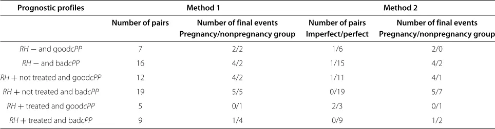
Table 4 Real data: number of pairs and final events according to the matching methods and to the six prognostic profiles
Prognostic profiles Method 1 Method 2
Number of pairs Number of final events Number of pairs Number of final events
Pregnancy/nonpregnancy group Imperfect/perfect Pregnancy/nonpregnancy group
RH−and goodcPP 7 2/2 1/6 2/0
RH−and badcPP 16 4/2 1/15 4/2
RH+not treated and goodcPP 12 4/2 1/11 4/1
RH+not treated and badcPP 19 5/5 0/19 5/7
RH+treated and goodcPP 5 0/1 2/3 0/1
RH+treated and badcPP 9 1/4 0/9 1/2
The number of imperfect pairs is also given for Method 2.
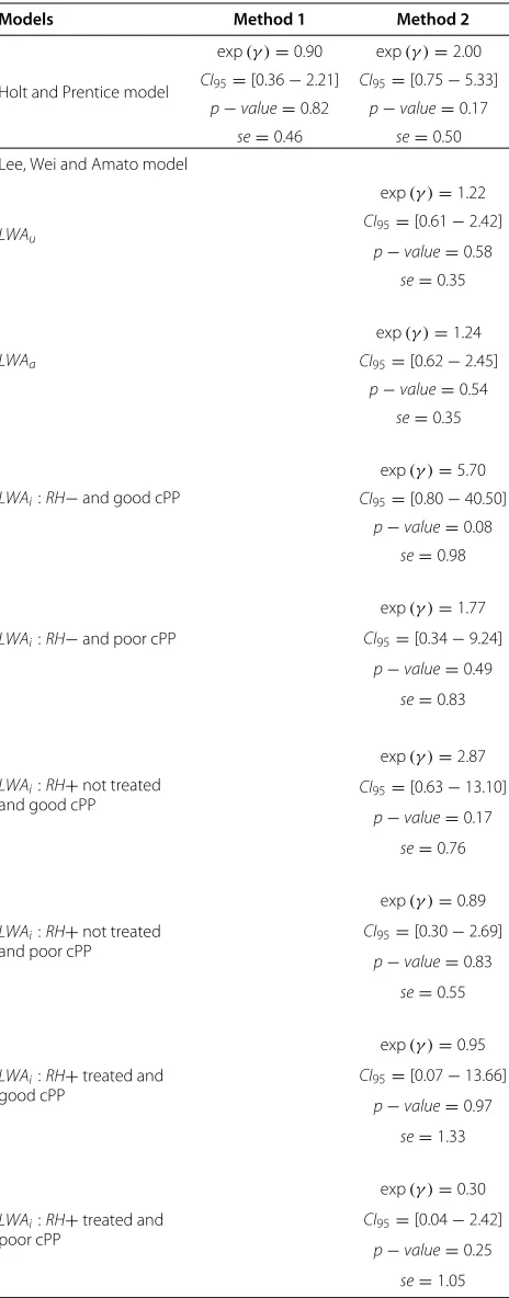
TheHPmodel applied with Method 1 yielded the fol-lowing estimations: exp(γ ) = 0.90,CI95% [0.36−2.21], not significant. Kranicket al.[5] and Veletgas et al.[4] concluded likewise as did Azimet al.[3], but the latter stratified their analysis on estrogen status. Other authors [7,10] found a protective role of pregnancy. All these authors used theHPmodel with Method 1 adjusted for the other known prognostic factors. In view of our simulation results, we believe that this estimation was underesti-mated and that the models should be used on censored correlated data created with Method 2. Regarding the lat-ter, theHPmodel yielded a larger value than with Method 1 but was still not significant (exp(γ ) = 2.00, CI95% [0.75− 5.33]). In view of our simulations, we conclude that HR(t) was widely underestimated with HP using Method 1 and only slightly underestimated withHPusing Method 2. The increasing value ofHR(t)estimated byHP between the two matching methods was not surprising. Method 2 and theLWAmodel, with or without adjusting for matching covariates (LWAuandLWAa), yielded simi-lar and not statistically significant results: exp(γ )=1.22, CI95%[0.61−2.42] and exp(γ )=1.24,CI95%[0.62−2.45], respectively. The difference inHR(t)values estimated by theHPandLWAumodels was not statistically significant. In such a context, we would like to estimate the proper effect of the subsequent pregnancy. It is more relevant to estimateHRa(t)thanHR(t). Even ifLWAishowed no significant interaction between the matching covariates and the pregnancy, because of the biological and clin-ical assumptions, we estimated the effect of pregnancy according to the six PP defined above using the LWAi model. Table 5 presents exp(γ )estimations according to the models and their 95% confidence intervals.
The apparent protective role of pregnancy for the the-oretically less favorable prognostic profile “RH+(treated or not) and poorcPP” and its increasing role in risk for the theoretically best prognostic profile “RH−and goodcPP” were surprising. There was no statistical significance, but it could be because of a lack of power of the combination Method 2 -LWAi.
Discussion
In our context of exposure occurring over time, we focused on two matching methods: Method 1, commonly used in the literature [3-5,7,10], and Method 2, our new approach. Method 1 composes the pairs in an a poste-riori way where the pairs are in fact considered to be known at diagnostic timet = 0. Method 2 creates pairs in “real-time”. Such matching designs create independence between pairs but dependence between the subjects of the same pair, and specific analytical methods exist for such a situation of correlated censored data. In our work we studied two semi-parametric models allowing for the stratified Holt and Prentice model [16] (HP) and the Lee, Wei and Amato model [20] (LWA). To estimate the aver-age exposure effectHR(t) and unlike the LWA, the HP did not make it possible to take into account either the matching covariates or the possible interaction between the matching covariates and the exposure.
The aim of this study was to analyze theHP andLWA models using the two matching methods in order to pro-pose the most efficient Method - Model combination to estimate and test the prognostic exposure effect HR(t) estimated through the models by exp(γ (t)).
In view of our simulations, the relative difference in the number of pairs between Method 1 and Method 2 depends on the ratioλ12(t) /λ13(t)and on the censoring percent. Compared to Method 1, the number of pairs was equal or larger with Method 2. In terms of bias andRMSE, Method 2 is more relevant than Method 1 to design the pairs, andLWAa is the best model for all the situations except when there is an interaction between the covari-ates and the exposure (β23 = β13), for which LWAi is more appropriate even if theHRi(t)estimations are not uniformly unbiased.
Table 5exp(γ )estimations and their 95% confidence
interval according to theHPandLWAmodels and to the
matching methods, with the p-value of the Wald’s Test
Models Method 1 Method 2
Holt and Prentice model
exp(γ )=0.90 CI95=[0.36−2.21]
p−value=0.82 se=0.46
exp(γ )=2.00 CI95=[0.75−5.33]
p−value=0.17 se=0.50 Lee, Wei and Amato model
LWAu
exp(γ )=1.22 CI95=[0.61−2.42]
p−value=0.58 se=0.35
LWAa
exp(γ )=1.24 CI95=[0.62−2.45]
p−value=0.54 se=0.35
LWAi:RH−and good cPP
exp(γ )=5.70 CI95=[0.80−40.50]
p−value=0.08 se=0.98
LWAi:RH−and poor cPP
exp(γ )=1.77 CI95=[0.34−9.24]
p−value=0.49 se=0.83
LWAi:RH+not treated and good cPP
exp(γ )=2.87 CI95=[0.63−13.10]
p−value=0.17 se=0.76
LWAi:RH+not treated and poor cPP
exp(γ )=0.89 CI95=[0.30−2.69]
p−value=0.83 se=0.55
LWAi:RH+treated and good cPP
exp(γ )=0.95 CI95=[0.07−13.66]
p−value=0.97 se=1.33
LWAi:RH+treated and poor cPP
exp(γ )=0.30 CI95=[0.04−2.42]
p−value=0.25 se=1.05
The estimation of the pregnancy effect standard error (se) by theHPandLWA
models are given.
gave the smallest estimation ofHR(t).HR(t)estimations were not statistically different from 1 withHP,LWAuand LWAa. According to biological and clinical hypothesis, we assumed that the effect of exposure was different accord-ing to the six prognostic profiles so we used the LWAi model. However, we did not conclude that pregnancy had neither a protective effect nor an adverse effect on pro-gression disease, even for women with positive hormonal receptors and poor clinical profile at diagnosis. Estimat-ing HR(t) by prognostic profiles using the combination Method 2 -LWAi, showed a different and opposite effect of exposure in the six health profiles, but none was sta-tistically significant. The sample size of the profiles was small and a few events occurred inside each profile, prob-ably leading to a lack of power of the combination Method 2 -LWAi.
Adjusting for the matching covariates and for their pos-sible interaction with exposure could be very interesting to interpret the effect of exposure HR(t). However, it could be more difficult with real data, especially in the event of multiple prognostic profiles. The sample had to be large enough to enable us to assess the performances of the models according to the two matching methods, especiallyLWAaandLWAi, which required a large num-ber of pairs. The erroneous estimation withLWAiin some extreme profiles could partially be explained as follows: in the “imperfect” pairs, we artificially prevent the non-exposed subject from having a final event, because she will first become an exposed subject of another pair. Maybe she will undergo the final event but as an exposed sub-ject and in another pair. Then, when the proportion of imperfect pairs is large, HRi(t) could be overestimated. Moreover the larger the ratioλ12(t) λ13(t), the larger the number of imperfect pairs, and the higher the overestima-tion ofHRi(t)and the faster its appearance. Owing to the values of theβuvk triplets chosen in the particular config-uration presented above, the subjects of the three profiles Z ∈ {(0, 0, 0),(1, 0, 0),(0, 1, 0)}experienced more expo-sure before any events, and simultaneously fewer events (before or after exposure), than the other PP. In these three profiles, the number of events in the exposed and in the non-exposed individuals is quite low, suggesting a possible lack of accuracy in the estimation ofHR(t). All the models needed enough pairs and enough final events to fit: the larger the number of imperfect pairs and the smaller the number of events, the worse the accuracy of the estimation ofHRi(t). In a future study, we will explore more deeply this problem of bias related to the percent of imperfect pairs in the sample.
subject. Concerning the management of the imperfect pair obtained with Method 2, the non-exposed subjecti of pair Pj was censored when she became the exposed subjectiof another pairPi at the timetEi; by
construc-tion, as said before, her exposure occurred before any other events. For LWA, an alternative would be to cen-sor the pairPj. Another alternative, whatever the model, would be to propose another non-exposed (perfect or imperfect) subject to the exposed subject of pairPj, who was now single in her pair. This issue deserves more investigation.
Using time intervals to estimate the effect of exposure as it changes over time was maybe not the most pertinent method, because it required many parameters. Therefore, to improve fitting, we intend to apply splines to fit the effect of exposure as it changes over time. Indeed, the present study sought to compare results of two known models devoted to censored correlated data, and the well-known frailty model was set aside because it requires the structure of correlation within the pairs to be specified. The next step would be to compare theHP,LWAand the frailty model using Method 2.
Conclusions
In conclusion, correlated censored data designing by Method 2 seems to be the more pertinent method to cre-ate pairs when the criterion which characterizes the pair is an exposure occurring over time. It would be inter-esting to estimate the proper effect of the subsequent pregnancy. It is then more pertinent to estimateHRa(t) thanHR(t). Thus,LWAaseems to be the best model for all the situations, except when there is an interaction between the covariates and the exposure, for whichLWAi is more appropriate, even if the estimations ofHRi(t)are not uni-formly unbiased.LWAa andLWAi gave a more accurate and relevant estimation of the effect of exposure in par-ticular context, where we can reasonably suppose that the latter depends on prognostic profiles.
Appendix A: Simulation of cohort data -Procedures and scenarios chosen
For each subject four independent times were generated: t12,t23,t13andC(censoring time), according to the inten-sities displayed in Table 2. From these times, 2 times of interest for each subject were derived: a time to expo-suret12 = tE and a time to final eventti. Two indicator variables were derived: E = 1 if an exposure occurs, 0 otherwise and= 1 if a final event occurs, 0 otherwise. Four possible quadruplets(tE;ti;E;)could be defined as follows:
(C;C; 0; 0)ifC <min(t12,t13), (t13;t13; 0; 1)ift13 ≤ min(t12,C),
(t12;C; 1; 0)ift12 <min(t13,C)andt12+t23>C, (t12;t12+t23; 1; 1)ift12 <t13andt12+t23≤C.
Such a design refers to an “illness-death” model with transition intensitiesλ12(t),λ13(t)andλ23(t)(Figure 1). All subjects were assumed to be in the initial state (state 1 or cancer diagnosis in our context) at time t = 0. They could move to the final state (state 3 or disease pro-gression) with a transition intensity λ13(t). They might undergo the intermediate event or exposure (state 2 or pregnancy) with intensityλ12(t), before developing any progression with intensityλ23(t). Date of entry into state 1 was chosen as time of origin for all transitions. Thus the parameter of interestHR(t)corresponded to the ratio λ23(t) /λ13(t). However, to computeλ23(t), we took into account the left truncation phenomenon: before being at risk of an event in the transition 2 → 3, a subject has to wait until its exposure occurs. This delayed entry leads the set of subjects at risk in transition 2 →3 to increase when an exposure occurs and to decrease when an event occurs. Thus the averageHR(t)is obtained from an exact formula involving the averages ofλ13(t)andλ23(t)which are computed through a numerical approximation (trans-formation of the time from continuous to discrete val-ues) (See the Appendix B). The average HR(t) adjusted for the different covariates was estimated empirically by using large size samples to guarantee good precision. Moreover, note that the larger the ratio λ12(t) /λ13(t), the larger the number of exposures in the simulated cohort.
The simulation model included (i) the choice of an instantaneous baseline risk functionλuv(t,Z)for each of the three transitionsu→v, (ii) the choice of theZeffects, exp(βuvk), for each transition and (iii) the choice for the censoring proportion.
For (i), an instantaneous average risk function λuv
t,Z=Zfor each of the three transitions was simu-lated: either a constant risk using an exponential density function(1), a monotone risk using a Weibull density function(2)or an increasing then decreasing risk using a loglogistic density function(3). Fiveλ
uv
t,Z=Ztriplets were simulated in order to construct five realistic con-figurations of HR(t): two constant, one increasing, one decreasing and one increasing then decreasing, where HR(t) range values were clinically pertinent (between 0.5 and 4 in the whole population). Table 2 displays the λuv
t,Z=Z distributions of each transition used for each of the five different configurations ofHR(t).
For (ii), different βuvk values for each of these five
λuv
Finally, for (iii), these previous 50 situations were first performed without censoring. To minimize simulations time, two levels of independent uniform censoring were implemented only with the followingβuvkscenario:β12= (−0.2,−0.4,−0.8),β13 = −β12andβ23 = β12; and they were applied to each of the five configurations ofHR(t). This yielded to 10 more situations (five HR(t) configu-rations with2 levels of censoring) for that βuvk scenario. The maximal event time tmax was set at 1000. The first uniform distribution for censoring time C was over the interval time [0;tmax], and the second one over [0; 2tmax]; then the maximal censoring time wasCmax = +∞,tmax or 2tmax. The overall censoring level was higher in the first censoring distribution but it also depended on theHR(t) configuration. In total we had50 situations without cen-soring and 10 with cencen-soring (the same five configurations with the two levels of censoring).
For each of the 60 situations, 1000 different data sets were generated with a sample size of 2000 subjects. Att= 0, these 2000 subjects were allocated to the eightZ pro-files. Att> 0, the 250 subjects of the 8 different profiles are divided up among the three transitions and change over time according to the fiveHR(t)configurations.
Appendix B: Calcul of the average exposure effect not adjusted for the covariatesHR(t)
Density functionf23(t), Repartition functionF23(t)and Survival functionS23(t)of transition 2 → 3 taking into account the left truncation
f23(t) = t
0
f23(t−u)f12(u)S13(u)du,
F23(t) = t
0
f23(v)dv= t
0 v
0
f23(v−u)f12(u)S13(u)du,
whereu is the exposure occurrence time andtthe final event time.
To obtain an useful formula we divide the time inKtiny intervals witht0<t1<· · ·<tk<· · ·<tK =Tmax
S23(tk)= k
j=1
1− f23
tj tj−tj−1 tj
0 f12(x)S13(x)dx−jl−=11
tl−tl−1
f23(tl)
= k
j=1
1− f23
tj tj−tj−1 tj
0 f12(x)S13(x)dx−lj−=11tl−tl−1f23(tl)
= k
j=1 ⎛ ⎜ ⎜ ⎜ ⎝ tj
0 f12(x)S13(x)dx− j l=1
tl−tl−1
f23(tl)
tj
0 f12(x)S13(x)dx− j−1
l=1
tl−tl−1f23(tl) ⎞ ⎟ ⎟ ⎟ ⎠ and
λ23(t)= −Log( S23(tk))
tk−tk−1 .
The average instantaneous hazardλ (¯ t)is equal to
¯
λ (t) =
zωz(t) λ (t|Z)
zωz(t)
ωz(t) = π (z)S(t|Z) ¯
ωz(t) = ωz( t)
zωz(t) ¯
λ (t) = z
¯
ωz(t) λ (t|Z)=
z ¯
ωz(t) λz(t)
¯
ωz(t) =
Nz(t)
z Nz(t)
whereλ (t|Z) = λz(t)is the average instantaneous haz-ard in the profilezat timet,Nz(t)is the number of subject at risk in the profilezat timet. Then we can write
HR(t)= λ23(t)
λ13(t) =
z
N23z(t)
z
N23z(t)λ23z(t)
N13z(t)
z
N13z(t)λ13z(t)
.
The computation ofNz(t)is the following.
In transition 1→3, a subject is at risk if it does not have any event and if it is not censored
N13z(t)=N13zS13z(t)G¯(t)S12z(t),
where
• S12z(t)is the survival rate in the transition1→2for the profilezat timet,
• S13z(t)is the survival rate in the transition1→3for the profilzat timet,
• N13zis the number of subject at risk in the profilezat timet=0,
• ¯G(t)=1−G(t)withG(t)is the repartition function of the variableCcharacterizing the censoring time. It does not depend on the profile.
In transition 2 → 3, taking into account the left trun-cation, a subject is at risk of event in this transition, if it entered in the transition and if it had neither an event nor being censored.
N23zcould be expressed as
N23z(t)= "
E23z(t)−D23z(t)−C23z(t) #
N23z
where
• E23z(t):the number of subjects which entered in the transition2→3in the time interval[0;t] ,
• D23z(t):the subjects which undergo the final event in the time interval[0;t] ,
• C23z(t):the censored subject in the time interval
[0;t] ,