A note on the graphical presentation of prediction intervals in random-effects meta-analyses

(1)

M E T H O D O L O G Y

Open Access

A note on the graphical presentation of

prediction intervals in random-effects

meta-analyses

Charlotte Guddat

1*

, Ulrich Grouven

1,2

, Ralf Bender

1,3

and Guido Skipka

1

Abstract

Background:Meta-analysis is used to combine the results of several related studies. Two different models are generally applied: the fixed-effect (FE) and random-effects (RE) models. Although the two approaches estimate different parameters (that is, the true effect versus the expected value of the distribution of true effects) in practice, the graphical presentation of results is the same for both models. This means that in forest plots of RE

meta-analyses, no estimate of the between-study variation is usually given graphically, even though it provides important information about the heterogeneity between the study effect sizes.

Findings:In addition to the point estimate of the between-study variation, a prediction interval (PI) can be used to determine the degree of heterogeneity, as it provides a region in which about 95% of the true study effects are expected to be found. To distinguish between the confidence interval (CI) for the average effect and the PI, it may also be helpful to include the latter interval in forest plots. We propose a new graphical presentation of the PI; in our method, the summary statistics in forest plots of RE meta-analyses include an additional row,‘95% prediction interval’, and the PI itself is presented in the form of a rectangle below the usual diamond illustrating the estimated average effect and its CI. We then compare this new graphical presentation of PIs with previous proposals by other authors. The way the PI is presented in forest plots is crucial. In previous proposals, the distinction between the CI and the PI has not been made clear, as both intervals have been illustrated either by a diamond or by extra lines added to the diamond, which may result in misinterpretation.

Conclusions:To distinguish graphically between the results of an FE and those of an RE meta-analysis, it is helpful to extend forest plots of the latter approach by including the PI. Clear presentation of the PI is necessary to avoid confusion with the CI of the average effect estimate.

Keywords:Meta-analysis, Heterogeneity, Random effects model, Forest plot, Prediction interval

Background

Using meta-analyses, the results of k studies related to the same question can be combined to produce an aver-age result. For example, in the context of clinical trials comparing a new pharmaceutical with a placebo, the treatment effect in each trial may be quantified by the odds ratio. Each of thekeffect estimates is recorded and finally summarized to one average estimate.

There are two different approaches in meta-analysis. The fixed-effects (FE) model assumes that the same treatment effect,θ, underlies all studies. Different esti-mates θ∧₁;. . .;θ∧_k for the true effect θ, resulting from thekstudies are expected to arise solely from sampling error. By contrast, the random-effects (RE) model incorporates the between-study variation, taking into account the heterogeneous true effects θ1;. . .;θk [1].

This model is appropriate when the observed

treatment effects between studies differ more from each other than would be expected from within-study variation alone. This heterogeneity between studies may arise from diversity in participants or

* Correspondence:[email protected]

1

Department of Medical Biometry, Institute for Quality and Efficiency in Health Care (IQWiG), Im Mediapark 8, Cologne 50670, Germany Full list of author information is available at the end of the article

(2)

interventions. The FE model can be viewed as a special case of the RE model, in which the between-study vari-ation is 0.

The parameter to be estimated depends on the ap-proach chosen. Under the assumption of a FE one true effect is estimated, whereas under the assumption of RE, the expected valueθ of the distribution of true effects is estimated. Despite this difference between the two approaches, both the graphical presentation and the in-terpretation of the results are in practice the same for

both models. The point and interval estimates of θ are

commonly displayed in a forest plot as a diamond, irre-spective of the model chosen [2-4]. Commonly used software packages in systematic reviews (for example, RevMan [5] in Cochrane reviews) do not distinguish be-tween the two models in the graphical presentation of results. Apart from a numerical value, the estimate of

the between-study variation, τ, is not shown in forest

plots of RE models.

The use of the prediction interval (PI) has recently been proposed to illustrate the degree of heterogeneity in for-ests plots of RE meta-analyses [6-8]. A PI provides a pre-dicted range for the true treatment effect in an individual study. Higginset al. [7] proposed using an additional hol-low diamond for the presentation of PIs, whereas Rileyet al. [8] added extra lines to the usual diamond of the effect estimate and its CI. For explanatory purposes, Borenstein et al. [9] displayed a bell-shaped curve, truncated at the limits of the PI, in accordance with the assumption of nor-mally distributed effects; however, to display the PI, they adopted the same graphical approach as the one proposed by Rileyet al. [8].

In this paper, we propose a new graphical approach for the presentation of PIs based on the original suggestion by Skipka [6], and compare it with the approaches of Higginset al. [7] and Rileyet al. [8].

Methods

Addressing heterogeneity in random-effects meta-analysis

The RE model assumes differences in the treatment

effects θi across k studies. Hence, the estimation and

presentation of the average effect and its CI alone are in-sufficient. It is also important to quantify the heterogen-eity between the effect sizes. The following measures are often used for this purpose: the between-study variance τ2_{, which can be estimated by various methods [10,11];}

the Q statistic, which is a measure of weighted squared

deviations; or I2, which describes the proportion of the total variance of the study effects due to heterogeneity [1,12,13]. One way to present the dispersion of the study effects graphically is to add the PI to the forest plot of RE meta-analyses.

Under the assumption that both the RE and the esti-mated average effect are approximately normally distrib-uted, that is:

θiNθ;τ2;θ ∧

N θ;SE θ∧ 2

!

;

Higginset al. [7] suggest that the PI is:

θ ∧

t1α=2;k2

ffiffiffiffiffiffiffiffiffiffiffiffiffiffiffiffiffi τ∧2_þ_SE∧

q

θ ∧ 2

;θþt1α=2;k2

ffiffiffiffiffiffiffiffiffiffiffiffiffiffiffiffiffi τ∧2_þ_SE∧

q

θ ∧ 2

" #

;

wheret1α=2;k2is the (1−α/2) quantile of the

t-distribu-tion withk-2degrees of freedom, andτ∧and SE∧ θ∧ de-note the estimated between-study variation and the standard error of θ∧ respectively. Applying at-distribution instead of a normal distribution reflects the uncertainty resulting from the estimation ofτ.

However, the assumption that the true effects are nor-mally distributed may not be justified. In these situations the choice of a different distribution [14] may be appro-priate, leading to a different PI.

In contrast to the commonly presented CI, which quantifies the precision of the estimated average effect, the PI includes the effect of an individual study, with the level of confidence (1 − α). It is important to note that the PI provides no information on the statistical signifi-cance ofθ∧.

The PI should be presented graphically in the forest plot of the RE meta-analyses. In such an extended forest plot, the degree of heterogeneity is illustrated, and a clear visual distinction is made between the results of the FE and the RE meta-analyses.

Modified extension of the forest plot

Forest plots are a graphical presentation of the results derived from a meta-analysis. They allow a rapid over-view of the potential heterogeneity of the studies ana-lyzed. In conventional forest plots, the effect measures of

the kstudies with the corresponding CI are represented

by a square with horizontal lines, in which the size of the squares reflects the weight that each study contributes to the meta-analysis. Below the results of the individual studies, the average estimate and its CI are displayed as a diamond, whose centre (vertical line) indicates the point estimate and whose width indicates the CI.

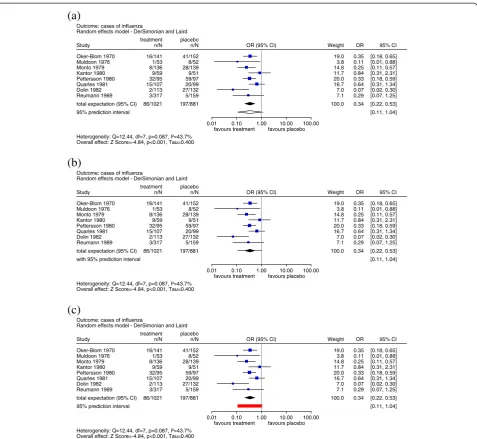
To date, the PI has not been part of the common lay-out of forest plots: However, some proposals to include PIs have been made. Figure 1a shows the proposal by Higginset al. [7], in which the PI is illustrated as a hol-low diamond. Riley et al. [8] suggest a different

presen-tation in which the confidence and PIs are ‘merged’

(3)

typical form of a diamond, and are then extended by lines on both sides representing the width of the PI. Bor-enstein et al. [9] displayed the PI in the same way and, for explanatory purposes, added a truncated bell-shaped curve based on the assumption of a normal distribution.

We propose an alternative graphical approach based on the original suggestion by Skipka [6], which can be considered a mixture of the approaches described. As

described previously, the row ‘total expectation (95%

CI)’represents the point and interval estimates for θ in

the form of a diamond. We have added a new row,‘95%

prediction interval’, to the forest plot, illustrating the

corresponding interval in an easily distinguishable way in the form of a rectangle (Figure 1c).

Results and discussion

The importance of the PI as a method to incorporate het-erogeneity in the presentation of RE meta-analyses has been discussed recently [16]. However, no transparent standard exists as to how to include PIs in forest plots. Higgins et al. [7] displayed the PI in the form of a dia-mond; that is, using the same symbol used to present the CI for the average effect. However, it could be misleading to use the same symbol for two different intervals. Riley

Oker-Blom 1970 16/141 41/152 19.0 0.35 [0.18, 0.65]

Muldoon 1976 1/53 8/52 3.8 0.11 [0.01, 0.88]

Monto 1979 8/136 28/139 14.8 0.25 [0.11, 0.57]

Kantor 1980 9/59 9/51 11.7 0.84 [0.31, 2.31]

Pettersson 1980 32/95 59/97 20.0 0.33 [0.18, 0.59]

Quarles 1981 15/107 20/99 16.7 0.64 [0.31, 1.34]

Dolin 1982 2/113 27/132 7.0 0.07 [0.02, 0.30]

Reumann 1989 3/317 5/159 7.1 0.29 [0.07, 1.25]

total expectation (95% CI) 86/1021 197/881 100.0 0.34 [0.22, 0.53]

95% prediction interval [0.11, 1.04]

0.01 0.10 1.00 10.00 100.00

Outcome: cases of influenza

Random effects model - DerSimonian and Laird

Heterogeneity: Q=12.44, df=7, p=0.087, I²=43.7% Overall effect: Z Score=-4.84, p<0.001, Tau=0.400

favours treatment favours placebo OR (95% CI)

Study n/N

treatment

n/N placebo

Weight OR 95% CI

Oker-Blom 1970 16/141 41/152 19.0 0.35 [0.18, 0.65]

Muldoon 1976 1/53 8/52 3.8 0.11 [0.01, 0.88]

Monto 1979 8/136 28/139 14.8 0.25 [0.11, 0.57]

Kantor 1980 9/59 9/51 11.7 0.84 [0.31, 2.31]

Pettersson 1980 32/95 59/97 20.0 0.33 [0.18, 0.59]

Quarles 1981 15/107 20/99 16.7 0.64 [0.31, 1.34]

Dolin 1982 2/113 27/132 7.0 0.07 [0.02, 0.30]

Reumann 1989 3/317 5/159 7.1 0.29 [0.07, 1.25]

with 95% prediction interval [0.11, 1.04]

0.01 0.10 1.00 10.00 100.00

Study n/N

treatment

n/N placebo

Weight OR 95% CI

Oker-Blom 1970 16/141 41/152 19.0 0.35 [0.18, 0.65]

Muldoon 1976 1/53 8/52 3.8 0.11 [0.01, 0.88]

Monto 1979 8/136 28/139 14.8 0.25 [0.11, 0.57]

Kantor 1980 9/59 9/51 11.7 0.84 [0.31, 2.31]

Pettersson 1980 32/95 59/97 20.0 0.33 [0.18, 0.59]

Quarles 1981 15/107 20/99 16.7 0.64 [0.31, 1.34]

Dolin 1982 2/113 27/132 7.0 0.07 [0.02, 0.30]

Reumann 1989 3/317 5/159 7.1 0.29 [0.07, 1.25]

95% prediction interval [0.11, 1.04]

0.01 0.10 1.00 10.00 100.00

Study n/N

treatment

n/N placebo

Weight OR 95% CI

(a)

(b)

(c)

Figure 1a) Implementation of the prediction interval in forest plots as suggested by Higgins_{et al}. [7]. b) Implementation of the

prediction interval in forest plots as suggested by Rileyet al.[8]. c) New implementation of the prediction interval in forest plots.

(4)

et al. [8] suggested plotting a combination of both inter-vals by adding extra lines to the left and right end of the diamond representing the average effect and its CI. This method of illustration makes it even more difficult to dis-tinguish between the CI and PI, and in addition, a line is already commonly used to present a CI.

To avoid such confusion, we recommend presenting the two intervals separately using different symbols. We sug-gest presenting the PI in an additional row of the forest plot in the form of a rectangle as originally proposed by Skipka [6]. The rationale for this is as follows: If we think of a set of infinitely large studies symbolized by squares in the corresponding forest plot, as already described, then because of the size of the studies, the horizontal lines representing the CIs converge towards zero. The disper-sion of the study effects becomes visible when the squares are merged, leading to the form of a rectangle. In contrast to the illustration by Borensteinet al. [9], this representa-tion of the PI can be used for any distriburepresenta-tional assump-tion whereas the bell-shaped curve can be applied only under the assumption of a normal distribution.

Note that Skipka [6] used the term ‘heterogeneity

interval’, rather than ‘PI’, because the interval describes the degree of heterogeneity between the studies. How-ever, because the interval provides the region in which, with high confidence, the true effect measure of a new study lies, the term‘prediction interval’may be more ap-propriate. Hunter and Schmidt [17] proposed a further term for what can be regarded as the predecessor of the PI; in the context of psychometric meta-analysis, they adopted the term‘credibility interval’, which‘contains the distribution of true effects and is roughly analogous to the prediction interval’[9].

We show the result of the same RE meta-analysis of eight studies investigating the effect of amantadine for the prevention of influenza [15], using the three approaches to present PIs described above (Figure 1). The estimated overall effect measured by the odds ratio for cases of influenza is 0.34, with a 95% CI ranging from 0.22 to 0.53. This interval is a measure of the pre-cision of the expected value of the distribution of true effects, and it depends heavily on the number of studies included in the meta-analysis. It would be incorrect to conclude that the effect in a newly conducted study will be within the interval of 0.22 and 0.53 with 95% confi-dence. On the other hand, the PI provides information about the distribution of effects. In this example, the results are heterogeneous, with τ∧¼0:4 (DerSimonian and Laird estimator [18]). The effect of a new study will be within an interval of 0.11 and 1.04 with 95% confi-dence. This is clearly shown in Figure 1c, thus avoiding misinterpretation, and represents our recommendation for the implementation of the PI in forest plots.

Conclusions

The investigation of potential heterogeneity is an im-portant task in meta-analysis. Various measures and stat-istical tests to assess heterogeneity have been suggested in the past [1,12,13]. Unfortunately, conventional forest plots fail to graphically present any measures related to heterogeneity. In addition, presenting the results of FE and RE models in the same way may convey the (incor-rect) impression that the two models estimate the same parameter. The inclusion of the PI in the graphical pres-entation of RE meta-analyses provides additional infor-mation about the variation of treatment effects. To graphically distinguish between the CI and PI in forest plots, it is important to choose a different form of illus-tration, for example, a rectangle instead of a diamond, as the latter symbol is commonly used to present the aver-age effect and its CI.

Competing interests

The authors declare that they have no competing interests.

Authors’contributions

GS wrote the initial draft of the manuscript, and CG, UG, and RB wrote the final manuscript. All authors read and approved the final version.

Acknowledgements

The authors thank the two referees for their helpful comments and suggestions. They also thank Natalie McGauran for editorial support.

Author details

1_{Department of Medical Biometry, Institute for Quality and Efficiency in}

Health Care (IQWiG), Im Mediapark 8, Cologne 50670, Germany.2Hannover Medical School, Hannover, Germany.3_{Faculty of Medicine, University of}

Cologne, Cologne, Germany.

Received: 28 March 2012 Accepted: 6 July 2012 Published: 28 July 2012

References

1. Higgins JPT, Thompson SG:Quantifying heterogeneity in a meta-analysis.

Stat Med2002,21:1539–1558.

2. Bourhis J, Overgaard J, Audry H, Ang KK, Saunders M, Bernier J, Horiot JC, Le Maitre A, Pajak TF, Poulsen MG,et al:Hyperfractionated or accelerated radiotherapy in head and neck cancer: a meta-analysis.Lancet2006,

368:843–854.

3. Hutton EK, Hassan ES:Late vs early clamping of the umbilical cord in full-term neonates: systematic review and meta-analysis of controlled trials.

JAMA2007,297:1241_–1252.

4. Nabi G, Cook J, N’Dow J, McClinton S:Outcomes of stenting after uncomplicated ureteroscopy: systematic review and meta-analysis.BMJ 2007,334:572.

5. The Cochrane Collaboration:Review Manager (RevMan): 5 for Windows edition. Oxford: The Cochrane Collaboration; 2008.

6. Skipka G:The inclusion of the estimated inter-study variation into forest plots for random effects meta-analysis - a suggestion for a graphical representation [abstract]. Dublin: XIV Cochrane Colloquium; 2006:23_–26. Program and Abstract Book; 2006:134.

7. Higgins JPT, Thompson SG, Spiegelhalter DJ:A re-evaluation of random-effects meta-analysis.J R Stat Soc A2009,172:137–159. 8. Riley RD, Higgins JPT, Deeks JJ:Interpretation of random effects

meta-analyses.BMJ2011,342:d549.

9. Borenstein M:Hedges LV, Higgins JPT, Rothstein HR: Introduction to meta-analysis. Chichester, UK: Wiley; 2009.

(5)

11. Knapp G, Biggerstaff BJ, Hartung J:Assessing the amount of heterogeneity in random-effects meta-analysis.Biom J2006,48:271–285.

12. Mittlböck M, Heinzl H:A simulation study comparing properties of heterogeneity measures in meta-analyses.Stat Med2006,25:4321–4333. 13. Biggerstaff BJ, Jackson D:The exact distribution of Cochran’s

heterogeneity statistic in one-way random effects meta-analysis.Stat Med2008,27:6093–6110.

14. Lee KJ, Thompson SG:Flexible parametric models for random-effects distributions.Stat Med2008,27:418–434.

15. Higgins JPT, Thompson SG, Deeks JJ, Altman DG:Measuring inconsistency in meta-analyses.BMJ2003,327:557–560.

16. Graham PL, Moran JL:Robust meta-analytic conclusions mandate the provision of prediction intervals in meta-analysis summaries.J Clin Epidemiol2012,65:503–510.

17. Hunter JE, Schmidt FL:Methods of Meta-Analysis: Correcting Error and Bias in Research Findings. 2nd edition. Thousand Oaks, CA: Sage Publications; 2004. 18. DerSimonian R, Laird NM:Meta-analysis in clinical trials.Control Clin Trials

1986,7:177–188.

doi:10.1186/2046-4053-1-34

Cite this article as:Guddatet al.:A note on the graphical presentation of prediction intervals in random-effects meta-analyses.Systematic Reviews20121:34.

Submit your next manuscript to BioMed Central and take full advantage of:

• Convenient online submission

• Thorough peer review

• No space constraints or color ﬁgure charges

• Immediate publication on acceptance

• Inclusion in PubMed, CAS, Scopus and Google Scholar

• Research which is freely available for redistribution