www.ann-geophys.net/25/1299/2007/ © European Geosciences Union 2007
Annales
Geophysicae
Recommendation for a set of solar EUV lines to be monitored for
aeronomy applications
J. Lilensten1, T. Dudok de Wit2, P.-O. Amblard3, J. Aboudarham4, F. Auch`ere5, and M. Kretzschmar6
1LPG, CNRS and Joseph Fourier University, Bˆatiment D de Physique, BP 53, 38041 Saint-Martin d’H`eres cedex 9, France 2LPCE, CNRS and University of Orl´eans, 3A Avenue de la Recherche Scientifique, 45071 Orl´eans cedex 2, France 3LIS, CNRS, 961 Rue de la Houille Blanche, BP 46, 38402 St. Martin d’H`eres cedex, France
4LESIA, Paris Observatory, 5 Place Jules Janssen, 92195 Meudon, France 5IAS, CNRS and Paris-Sud University, Bt. 121, 92405 Orsay cedex, France
6SIDC, Royal Observatory of Belgium, Avenue Circulaire 3, 1180 Brussels, Belgium
Received: 7 November 2006 – Revised: 15 April 2007 – Accepted: 7 May 2007 – Published: 29 June 2007
Abstract. In two recent studies, Dudok de Wit et al. (2005) and Kretzschmar et al. (2006) have shown that the solar Ultra-Violet spectrum between 25 and 195 nm can be recon-structed from the observation of a set of 6 to 10 carefully chosen spectral lines. The best set of lines, however, is appli-cation dependent. In this study, we demonstrate that a good candidate for aeronomy applications consists of the follow-ing 6 lines: H I at 102.572 nm, C III at 97.702 nm, O V at 62.973 nm, He I at 58.433 nm, Fe XV at 28.415 nm and He II at 30.378 nm. The TRANSCAR model is used to quantify the impact of each individual line on the density, temperature and velocity profiles. Using a multidimensional scaling tech-nique, we show how to select from this the best set of lines. Although this selection is motivated by the specification of the ionosphere, our set of lines is also found to be appro-priate for reconstructing the variability of the solar spectrum between 25 and 195 nm.
Keywords. Ionosphere (Modeling and forecasting; Solar ra-diation and cosmic ray effects) – Solar physics, astrophysics, and astronomy (Ultraviolet emissions)
1 Introduction
The continuous monitoring and the real-time estimation of the solar irradiance in the X-ray (XUV, from 1 to 10 nm) and Extreme Ultraviolet (EUV, from 10 to 121 nm) spectral bands is a crucial issue in space weather. The prime applica-tion is orbitography.The XUV/EUV flux is the main energy input for thermosphere/ionosphere system. Sudden increases
Correspondence to: J. Lilensten
in the flux heat the thermosphere, cause it to expand, which, in turn, increases the friction for low orbit spacecraft. The consequence is altitude loss and orbital acceleration. The specification of the thermosphere is also needed for the local-ization of space debris. A second important group of users is telecommunications and positioning, including ground-space and ground-space to ground-space communications. The ionosphere acts as a filter for electromagnetic waves, so that sudden changes in solar activity also result in a degradation of the positioning and perturbations (or even loss) of communica-tions.
The solar XUV/EUV flux is very variable and is primarily governed by solar magnetic activity.
– Short-term variations (on scales of minutes to hours) are related to solar eruptive phenomena.
– Intermediate term variations, modulated by the 27-day rotation period of the Sun, are related to the appearance and disappearance of active regions, plages, network and coronal holes on the solar disk.
– Long-term variability is related to the 22-year magnetic cycle of the Sun.
As of today, there has been no permanent monitoring of the solar XUV/EUV irradiance with sufficient radiometric accu-racy (<10%) and over more than one solar cycle. Most mis-sions have either provided high spectral resolution with little temporal coverage, or the converse. This has resulted in a large EUV hole (Woods et al., 2005) that has only ended in 2002.
1300 J. Lilensten et al.: Monitoring the solar EUV flux for aeronomy Since that time, however, there have only been a few
oc-casional solar XUV/EUV irradiance measurements, such as the San Marco 5 satellite (Schmidtke et al., 1992; Tobiska et al., 1993) and several sounding rockets. Moreover, for wavelengths short of 110 nm, no space-borne spectrograph has been calibrated in-flight. Continuous measurements have started again in the 1990s with the Solar EUV Monitor (SEM) on board SOHO (Judge et al., 1998), the Upper At-mosphere Research Satellite (UARS; Woods et al., 1996) and the Solar Radiation & Climate Experiment (SORCE; Rottman, 2005). Unfortunately, these measurements are of little use for aeronomy, as they are either broadband (SEM) or do not properly cover the EUV range (SEM and UARS).
Due to the lack of adequate irradiance data, most thermo-sphere/ionosphere models rely today on proxies for the solar irradiance, such as thef10.7index (radio flux at 10.7 cm) or the magnesium line Mg II K (Heath and Schlesinger, 1986). The solar radio emission at 10.7 cm is generated by a variety of physical processes that occur from the solar corona down to the photosphere. Although this parameter correlates rea-sonably well with the solar XUV/EUV flux, it clearly cannot replace it. Several other proxies have been developed, but none of them can be used as a substitute for the irradiance (Floyd et al., 2005).
Continuous and spectrally resolved measurements of the solar EUV irradiance resumed in February 2002 with the So-lar EUV Experiment (SEE) grating spectrograph on board the TIMED satellite (Woods et al., 2005). The prime science objective of the TIMED mission is to understand the energy transfer into and out of the Mesosphere and Lower Thermo-sphere/Ionosphere (MLTI) region of the Earth’s atmosphere, and the basic structures that result from the energy transfer into these regions. The SEE suite consists of a spectrograph and a series of photometers designed to measure solar ultra-violet radiation from 0.1 to 194 nm.
Using a statistical analysis of 2 years of SEE data, Dudok de Wit et al. (2005) have shown that it is possible to recon-struct the full XUV/EUV spectrum from a linear combination of 6 to 10 spectral lines only, with an accuracy better than 5%. It is interesting to note that the same small sets of lines had been identified earlier by using a different method. Kret-zschmar et al. (2004) used a broad set of optically thin lines measured by the SUMER (Solar Ultraviolet Measurements of Emitted Radiation) instrument on board SOHO to com-pute a mean Differential Emission Measure (DEM), which was then inverted. This resulted in a reference spectrum for the quiet Sun. Using this physical approach, Kretzschmar et al. (2006) were able to retrieve the whole irradiance spec-trum from the observation of 6 reference lines.
In both approaches, the choice of the most appropriate lines is application dependent. For aeronomy, the prime ob-jective is the specification of the thermosphere/ionosphere system, whereas in solar physics, the reconstruction of the spectrum matters more. Dudok de Wit et al. (2005) provide a methodology for selecting the best set of lines; here we use
the same approach to determine which set of lines is most appropriate for aeronomy purposes. Due to the lack of ob-servational data, we use the TRANSCAR ionospheric model (Diloy et al., 1996) to quantify the impact of each individ-ual spectral line on the plasma parameters. We only con-sider the EUV range, since this has the strongest impact on the thermosphere/ionosphere system. The solar irradiance in the XUV and UV is also of importance for space weather (Danilov, 2006), impacting, for example, the ozone concen-tration in the lower mesosphere and in the upper stratosphere (Rozanov et al., 2005). These effects, however, occur at al-titudes far below the ones we are interested in (typically be-tween 100 and 800 km), in which satellite drag is an impor-tant issue.
2 Description of the method
Particle populations in the ionosphere can be conveniently split into a large thermal Maxwellian population and a small non-thermal one. Each ion species, however, has its own distribution, which differs from that of the electrons. The processes which drive these populations are strongly time-dependent, as they are governed by chemical reactions, by collision frequencies, by the dynamics (neutral winds), etc; a time-dependant fluid description is required to properly de-scribe the behaviour of these populations.
The hottest population mainly consists of electrons with non-Maxwellian distributions, whose energy exceeds the mean thermal energy by orders of magnitude. Their energy source is located either in the magnetosphere (electron and proton precipitations) or in the atmosphere (photoionization). Each primary particle can cause many ionizations and exci-tations. Transport, however, is fast enough to be considered as instantaneous versus the characteristic time scale of the precipitation event or the solar event. This means that non-thermal particles can be adequately described by a steady-state kinetic description.
the heating rates, which, in turn, feed the fluid part of the model.
The fluid part of TRANSCAR is based on an eighth-moment approximation of Boltzmann’s equation (Schunk and Nagy, 2004). The resulting set of equations, projected along the direction of the magnetic field, allows one to deter-mine the density, velocity, temperature and heat flow for each ion species. Electron density and velocity profiles are esti-mated assuming charge neutrality and ambipolar flow, while taking into account the effect of the electric field. TRAN-SCAR describes the ionosphere from 100 up to 3000 km, solving the set of equations for molecular and for atomic ions. In this paper, we restrict our study to altitudes below 800 km, where most of the production by photoionization oc-curs.
To summarize, the main inputs we use here are the spec-trally resolved EUV flux and the neutral atmosphere, while the main outputs are the electron and ion production rates, concentrations, temperatures and velocity profiles between 100 and 800 km.
3 Description of the XUV/EUV flux
Most of the current EUV / XUV models rely on a few exper-iments made by the Atmospheric Explorer missions (Hin-teregger, 1981) and by rocket flights. Hinteregger (1981) and Hinteregger and Katsura (1981) gave a first represen-tation of solar XUV/EUV fluxes for aeronomical applica-tions. A first reference flux SC#21REF was assembled from measurements performed in July 1976 (f10.7=70), and given in 1659 wavelengths. Torr and Torr (1979) and Torr and Torr (1985) later proposed two reference fluxes for aeron-omy called F79050N (f10.7=243) and SC#21REF (f10.7=68). Their UV spectrum was divided into 39 bins, some of which correspond to intense spectral lines: He II and Si X at 25.63 nm, Fe XV at 28.415 nm, Si XI at 30.331 nm, He II at 30.378 nm, Mg IX at 36.807 nm, Ne VII at 46.522 nm, OVI at 55.437 nm, He I at 58.433 nm, Mg X at 60.976 nm, O V at 62.973 nm, O III at 70.331 nm, N IV at 76.515 nm, Ne VIII at 77.041 nm, O IV at 78.936 nm, C III at 97.702 nm, H I at 102.572 nm (Lymanα) and finally O VI at 103.191 nm. The Lyαline at 121.565 nm does not appear in this list be-cause it is not energetic enough to ionise the terrestrial ther-mosphere. For terrestrial aeronomy, O VI is not energetic enough either, which leaves us with 16 pertinent lines only. The remaining boxes represent the mixing of close lines and the continuum. This work turned out to be extremely use-ful, partly because the authors proposed the corresponding absorption and ionisation cross sections for the major ther-mospheric species. Most of the current aeronomic calcu-lations are still based on this set of 39 lines, whose wave-lengths (respectively energies) range from 2.37 nm (532 eV) to 103.191 nm (12.015 eV), thus covering the XUV and EUV parts of the solar spectrum.
The above-mentioned reference fluxes have proven to be sufficiently accurate for most applications and so existing models are very unlikely to be modified in a near future to take into account other lines. For that reason, we shall also restrict ourselves here to the 16 most intense lines of this set. One of the questions to be addressed below is whether this set of lines is sufficiently informative, i.e. whether the full XUV/EUV spectrum can be reconstructed from it.
Several authors have developed new models to take better advantage of the AE database. Tobiska (1991) and Tobiska and Eparvier (1998) developed a model called EUV, which takes data from satellites, rockets and ground-based facili-ties. The more recent SOLAR2000 model provides several indices that are tailored to specific needs, such as the S10.7 index for the specification of the neutral density (Tobiska and Nusinov, 2006). These quantities, however, may not be considered as indices, since they result from a computation and not from direct observations (Lathuill`ere and Menvielle, 2004). Another improved model is EUVAC (EUV for Aero-nomic Calculations) (Richards et al., 1994), which differs from the previous ones by the choice of the reference flux, and the interpolation formula.
For the present study, we use Torr and Torr’s model, as its dependence on solar activity is governed byf10.7only and not the date. To emphasize the effects of the lines, we use the reference flux F79050N, which corresponds to a very ac-tive Sun (f10.7=243). Wavelengths greater than 103.191 nm (and especially Lyαat 121.565 nm) are not considered here, since they cannot ionize from the ground. Such wavelengths are nevertheless important because they dissociate heat the thermosphere. The ion densities are affected by the Lyαline and the continuum above it because of the molecule destruc-tion. The temperature is affected because of heating. For all these effects, however, have been compared with our calcu-lations using various instruments. We compared ion/electron densities and temperatures (Diloy et al., 1996) and conduc-tivities (Lilensten et al., 1996) with the EISCAT incoherent scatter radar; emission rates were investigated with optical facilities (Witasse et al., 1999) and in different geomagnetic conditions (Blelly et al., 2005). All these comparisons, the impact falls within the instrumental error bars. Although this is not a reason to exclude longer wavelengths in the future, it justifies the choice of a reduced spectral range in the present study.
Let us also mention that the Lyαline at 102.5 nm can ion-ize NO and all the neutral mesospheric constituents, and that the wavelengths short of about 2 nm have an important im-pact on the D region. These effects should be taken into ac-count in the study of altitudes below 100 km.
4 Effect of the spectrum on the ionosphere
1302 J. Lilensten et al.: Monitoring the solar EUV flux for aeronomy
Fig. 1. State of the ionosphere under quiet conditions, as obtained from the TRANSCAR model with: the ion density profile (left panel, the
black curve refers to the total density), the ion velocity profile (middle panel) and the electron temperature profile (right panel).
Fig. 2. Electron production rate associated with the continuum (dashed line) and the set of 16 spectral lines used in XUV/EUV aeronomical models (thin full line). The total production is shown in a thick full line.
order to focus on the effect on the production rates and the densities. This choice does not have strong implications on our conclusions. The relative intensity of the lines does, of course, vary in time (Schwenn, 2006), as coronal emissions are more strongly modulated by the solar cycle than chromo-spheric emissions. The altitude, however, where the energy is deposited, does not change drastically, and the ratios between chromospheric and coronal solar lines do not vary enough to invert our conclusions.
We model the electron production rate at mid-latitude (45◦ geographic latitude), at local noon for day 180 (i.e. mid-June). The F region peaks at 280 km, with O+ being as usual the dominant ion in that region and NO+/O2+ the dominant ones in the lower F and E regions.
[image:4.595.58.277.379.526.2]The continuum accounts for approximately one half of the total production at low altitude (below 125 km) and slightly more above; neither the continuum nor the spectral lines may therefore be neglected.
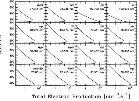
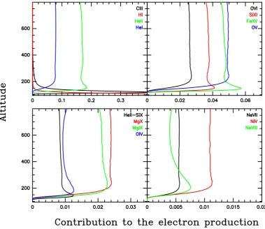
4.2 Effect of the different lines on the electron production To determine the electron production associated with each of the 16 spectral lines, we simply run the kinetic part of TRANSCAR with each single line turned on individually and the rest of the spectrum, including the continuum, turned off. In doing so, we can precisely determine where the energy is deposited. Figure 3 shows the electron production rate as-sociated with each line, while Fig. 4 displays the production ratio.
From Fig. 4, we can see that He II contributes to about 20% of the total electron production above about 150 km, while H I and C III produce, respectively, about 40% at 100 km and 20% at 120 km. These 3 lines are the most im-portant ones for monitoring the electron production. 4.3 Effect of the different lines on densities and
tempera-tures
While the electron production rate can easily be determined by turning on each spectral line individually, this procedure does not apply anymore for macroscopic parameters. Indeed, if we turn on a single line, a thin slab will be ionized and heated, creating large and totally unrealistic temperature and production gradients. The system then becomes discontin-uous and the differential fluid transport equations cannot be solved anymore. Therefore, to study the effect of a given wavelengthλon an ionospheric parameterX(density, tem-perature or velocity), we do the opposite and turn on all but one spectral line. Next we compute the relative contribution of that spectral line as a function of altitudeh
Rλ(h)=
Xfull(h)−Xλ(h) Xfull(h)
,
whereXfull(h)is the result obtained with the full Sun condi-tions (i.e. no lines turned off), andXλ(h)the result obtained with lineλturned off. This method supposes that the con-tributions of the lines are weak enough for the effects to be linear. To check this, we successively computed the relative contributionRλ(h)for two intense lines: He II (30.378 nm) and C III (97.702 nm). These lines were first turned on and then turned off simultaneously. The impact on the production rate is illustrated in Fig. 5, which shows the production rate. We indeed find that the production rate of the sum equals the sum of the production rates. The discrepancy is largest around 150 km, where it remains below 3%; the resolution of the plot does not allow one to see it. We can therefore safely assume that the production rate is linear in the param-eters versus the wavelengths. The same conclusion holds for the density and the temperature.
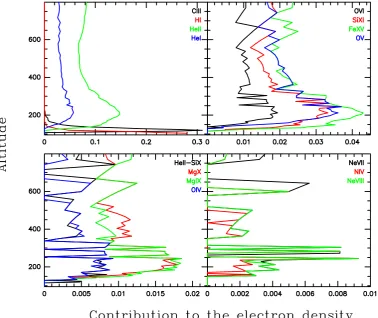
The relative contribution of each spectral line to the elec-tron density, the elecelec-tron temperature and the velocity are, respectively, displayed in Figs. 6 to 8. The H I lines produce about 30% of the electrons around 100 km but have very lit-tle impact on the temperature or on the dynamics, see Fig. 6. The C III line is the most important one around 110 km. H I, together with C III, are key lines for monitoring the E and lower F regions. He II is the main production line at 150 km, and is also a dominant source of energy for the electron den-sity at higher altitudes. O V is acting very efficiently above 200 km, as well as He I. Note, however, that several lines lead to similar profiles. The deposition profiles of Fe XV and Si XI, for example, are very similar in shape. The impacts of O V, Fe XV and Si XI on the density are much alike, as are the temperature responses to Fe XV and Si XI. In the next section, we shall provide a method for eliminating lines that have redundant signatures.
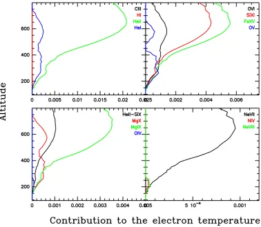
The lines that mostly impact the temperature (see Fig. 7) are again He II, but also Fe XV and Si XI. These are also the most intense amongst the energetic lines. Note that the sum of all the contributions is not equal to one. Several phe-nomena influence the temperature of the ionosphere through various energetic couplings: frictional heating of the atmo-sphere, thermalisation of the photoelectrons, energy transfer by thermalisation of the precipitating electrons, and energy input by a downward electron heat flow. Frictional electron heating is negligible because of the small electron mass. The main source of energy comes from suprathermal electrons. The energy transfer to thermal electrons (Swartz and Nis-bet, 1972) is particularly efficient at low energies, typically below 10 eV. To obtain these low energy electrons to heat the thermal bulk, it is necessary either to ionize the neutrals with energies close to the ionization threshold (typically be-low 22 eV or wavelengths above 55 nm), or to produce many energetic primary electrons. In the first case, the primary electrons have little energy, as they are created with the en-ergy of the incident photon minus the ionization threshold (about 13 eV). At these energies, however, the excitation is also very efficient; such photons can generate several elec-trons, thus producing some electron heating. In this aspect, the continuum heats the ionosphere more efficiently than the lines. In the second case (with high energy photons), ioniza-tion is much more efficient than excitaioniza-tion. Many primary electrons are generated, which can produce secondary elec-tons of any energy (including low ones) through collisions with neutrals. Secondary electrons with energies typically below 10 eV start heating the ambient thermal electrons. At higher energies, most of the solar irradiance is already con-tained in the continuum of the current models. This explains the results shown in Fig. 7.
1304 J. Lilensten et al.: Monitoring the solar EUV flux for aeronomy
Fig. 3. Electron production rate associated with each of the 16 spectral lines versus altitude in km.
and O2, or the atomic oxygen to the 1-D state, or the fine structure levels of O. These processes are detailed in the book by Schunk and Nagy (2004).
The effect of the solar XUV/EUV on the velocities is not shown here. The reason is as explained above: the regular XUV/EUV flux is not the main driver of the ionospheric ve-locities. Our calculation only shows that, as for the densities, C III is a good monitor for the F1 region while He II is better for the topside. In between, Fe XV constitutes a good link.
From these considerations, we conclude that the nonre-dundant set of lines that mostly impact the ionosphere at dif-ferent altitudes are H I at 102.572 nm, C III at 97.702 nm, O V at 62.973 nm, He I at 58.433 nm, Fe XV at 28.415 nm, Si XI at 30.331 nm, and He II at 30.378 nm. Since, how-ever, the impact of Fe XV and Si XI is very similar in terms of electron production and temperature profile, we eliminate the weakest of the two, which is Si XI. As shown in Fig. 2, these discrete lines account for about only half of the electron and ion production.
5 A different procedure for selecting the best lines
Our objective now is to find a procedure for selecting those lines that significantly impact the electron density, tempera-ture or productions profiles. This set of lines must be com-plete enough to allow for the reconstruction of the various profiles that can be generated by the full XUV/EUV spec-trum. When several lines give rise to the same profile, how-ever, only one (in general the strongest one or the one that is easiest to measure) should be retained. This is an opti-mization problem, for which insight can be gained from a so-called connectivity map. We use the technique that was introduced by Dudok de Wit et al. (2005) for reconstructing the solar XUV/EUV spectrum from a small set of lines. Let us consider, for example, the density profile. Two spectral lines are considered to be dissimilar if their impacts on the density profile differ; two profiles are on the contrary similar if the profile changes are the same.
Fig. 4. Relative contribution of each spectral line to the total electron production versus the altitude in km.
δ(λ1, λ2)= s
Z
Xλ1(h)−Xλ2(h)
2
dh,
whereXstands either for the relative change in density, tem-perature or production rate; each parameter is integrated from 100 up to 400 km. We now want to represent the dissimilar-ity between spectral lines as distances in a low-dimensional space (called connectivity map), in order to make the data accessible to visual inspection and exploration. To do so, we represent each spectral line by a single point in a multi-dimensional space, in such a way that the distance between each pair of lines equals the distanceδ(λ1, λ2)defined above. The closer two lines are, the more similar their impact on the profile of parameter X is. The dimensionality of this space, in principle, equals 15, i.e. the number of lines minus one. Since, however, many lines have similar signatures, a projec-tion onto a lower-dimensional space can easily be carried out, while preserving the distances. The appropriate technique for doing such a projection is multidimensional scaling (Borg and Groenen, 1997). In our particular case, the projections in different directions are closely connected to the principal axes of the data (Chatfield and Collins, 1995). Using the
Sin-Fig. 5. Linearity check of the impact of the He II and C III lines on
the electron production rate. The thick full lines represent the sum of the contributions of He II and C III, the thin line the contribution of He II and the dashed line the contribution of C III.
[image:7.595.316.540.443.587.2]1306 J. Lilensten et al.: Monitoring the solar EUV flux for aeronomy
Fig. 6. Relative contribution of the different XUV/EUV lines to the total electron density versus latitude in km. Notice that the scales of the
abscissa vary by more than one order of magnitude. Discretization effects show up at very low electron densities.
Xλ(h)= 16 X
k=1
Akfk(h)gk(λ) ,
with the orthonormality constraint
hfk(h)fl(h)i = hgk(λ)gl(λ)i =δkl,
whereh· · ·imeans ensemble averaging. The weights are tra-ditionally sorted in decreasing orderA1≥A2≥. . .≥A16≥0. The number of modes equals the number of spectral lines. Large weights correspond to modes that describe features shared by many lines. The proportion of variance accounted for by the firstimodes is
Vi = Pi
k=1A2k P16
k=1A2k .
In our case, two to three modes are enough to describe over 95% of the variance. This important result considerably eases the analysis, since it allows us to determine the salient features of the dissimilarity by using a three-dimensional projection. The coordinates of the spectral lines along the
i-th axis of the connectivity map are given byAigi(λ). Let
us stress that the axes of this connectivity do not convey here any clear physical meaning; what matters is the relative dis-tance only between spectral lines.
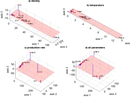
Figure 8 shows the location of the 16 lines in a three-dimensional space, for each of the physical parameters in-dividually, and for all three together. The origin corresponds to the full spectrum, with no lines turned off. Adding a fourth dimension to these plots does not add pertinent information and merely complicates the visualisation.
Fig. 7. Relative contribution of the different XUV/EUV lines to the electron temperature. The scales of the abscissa varies from one plot to
the other.
candidates for modelling density changes are the H I, C III and He II lines.
Figure 8b shows the impact on the temperature profile and reveals a different ordering of the spectral lines, with a preva-lence of energetic lines. H I and C III now have little impact, while He II is still as strong, followed by Fe XV, Si XI and Mg IX. Note also that the lines are essentially distributed in a two-dimensional space, as the third dimension conveys little information. There is indeed more redundancy in tempera-ture profile changes than in density or production rate pro-files.
The impact on the production rate (see Fig. 8c) again re-veals a different ordering, with four groups of lines. In this figure, we encounter again H I, C III and He II, each of which leads to a different profile. The remaining lines are clus-tered together and could be represented by Fe XV only. One can finally analyse all three parameters (density, temperature and production rate) together, which gives the plot shown in Fig. 8d. This figure is a weighted average of the previous ones, showing again the predominance of He II, C III, H I, followed by a bunch of other weaker lines such as Fe XV, He I, etc.
1308 J. Lilensten et al.: Monitoring the solar EUV flux for aeronomy
Fig. 8. Three-dimensional connectivity map of the spectral lines, in which the distance between each pair of lines reflects their degree of
dissimilarity. The maps correspond to the density profile (a), the temperature profile (b), the production rate (c), and all three parameters together (d). Vertical bars are there merely as a guide to locate the lines with respect to the plane with vertical coordinatez=0 (shown in translucent red). Only those lines are labeled, which sufficiently stand out of the clusters of points.
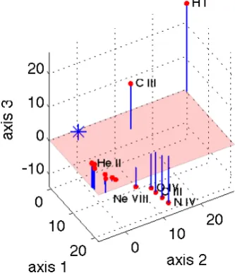
We conclude from Figs. 8 and 9 that the best set of lines for describing the variability of our ionospheric parameters are: H I (102.572 nm), C III (97.702 nm) and He II (30.378 nm), followed by series of less influential lines such as Fe XV (28.415 nm), He I (58.433 nm) and O V (62.973 nm). The first three lines are mandatory, while the choice of the latter three could be adapted, for example, to instrumental con-straints. We conclude that a dedicated instrument, which continuously measures the absolute irradiance of those 6 lines, would provide all the information that is needed to specify the ionospheric response to the full solar XUV/EUV spectrum. Other inputs have to be added to this list if one aims to model effects such as particle precipitation. Let us stress, however, that in terms of space weather applica-tions, the XUV/EUV spectrum is the prime quantity for iono-spheric specification.
Our results apply to stationary regimes. In the case of an eruptive event, the sudden enhancement of the flux results in a transitory regime for which our set of lines may not be
opti-mal anymore. Since, however, our set covers regions ranging from the chromosphere up to the hot corona, the spectrum of eruptive phenomena should still be properly covered by it.
6 Retrieving the full spectrum from these 6 selected lines
Fig. 9. Same plot as Fig. 8d, after normalizing each quantity to its
standard deviation.
each spectral bin between 27 and 194 nm can be expressed as a linear combination of our 6 spectral lines. The feasibility of such a reconstruction is indeed suggested by the high correla-tion between irradiances measured at different wavelengths, and has been confirmed by Dudok de Wit et al. (2005).
Here we use one year of TIMED spectra (i.e. the period spanning from February 2002 till February 2003) to estimate the coefficients needed for reconstructing the flux at all wave-lengths from our six lines, and use the remaining three years to compare the fitted flux against the true one. Since priority is given to the reconstruction of the spectrally resolved irra-diance rather than to the shape of the spectrum, our global error criterion is
X= q
P λ
P
t[X(t, λ)−Xfit(t, λ)]2 q
P λ
P
tX2(t, λ) ,
whereX(t, λ)is the flux at timetand wavelengthλ. From our calculation, the relative global errorXfor our set of lines is 6.8%, to be compared with the best combina-tion of 6 lines, which yieldsX=3.7%. It comes as a surprise that the best set of lines for aeronomy is so close to the best set of lines for reconstructing the XUV/EUV spectrum. The selection criteria are indeed totally different. One possible reason for this agreement is that both approaches lead to sets of lines that issue from different layers of the solar atmo-sphere. These lines, in addition, are quite evenly distributed in the EUV range of wavelengths, making them good candi-dates both for 1) representing the dynamics of the solar EUV spectrum at different wavelengths and 2) estimating the im-pact on the thermosphere/ionosphere system at different alti-tudes. A direct consequence of this result is the absence of a need for explicitly monitoring the (non-negligible)
contri-Table 1. The six lines that allow one to specify the ionospheric
density, temperature and electron production rate.
Mandatory lines H I 102.572 nm C III 97.702 nm He II 30.378 nm
Less influential lines Fe XV 28.415 nm He I 58.433 nm O V 62.973 nm
bution of the continuum, as it is already properly taken into account by the spectral lines.
7 Conclusion
The objective of this study was to determine whether an iono-spheric specification model could use as solar input a small set of spectral lines rather than using the full solar XUV/EUV spectrum. Using TRANSCAR to model the impact of var-ious XUV/EUV lines on three ionospheric parameters (the density profile, the temperature profile and the production rate profile), we find that six lines are sufficient to reproduce the variability of the XUV/EUV spectrum. The solution con-sists of a selection procedure based on a statistical technique called multidimensional scaling, which allows one to elim-inate lines that have a similar impact on the ionosphere in terms of amplitude and profile change.
A direct application of this study is the real-time speci-fication of the ionosphere/thermosphere system. For space weather purposes, it would indeed be much more convenient to have a small dedicated instrument that continuously mea-sures the absolute intensity of a few lines or a few spectral bands, rather than a full-fledged spectograph, which is more appropriate for fundamental science. The LYRA radiome-ter (Hochedez et al., 2006) on board the PROBA2 satellite, which is due for launch in 2008, will provide experimen-tal ground to our approach. LYRA will continuously mea-sure the EUV/UV spectrum in 4 bands: 1–20 nm, 17–70 nm, 115–125 nm and 200–220 nm. Although the choice of these spectral bands was technology-driven, LYRA will provide the first opportunity to test our spectral reconstruction ap-proach.
Acknowledgements. We thank the COST 724 action for financial and scientific support.
Topical Editor M. Pinnock thanks two anonymous referees for their help in evaluating this paper.
References
Blelly, P.-L., Lilensten, J., Robineau, A., Fontanari, J., and Alcayd´e, D.: Calibration of a numerical ionospheric model with EISCAT observations, Ann. Geophys., 14, 1375–1390, 1996,
[image:11.595.339.517.99.177.2]1310 J. Lilensten et al.: Monitoring the solar EUV flux for aeronomy
Blelly, P.-L., Lathuill`ere, C., Emery, B., Lilensten, J., Fontanari, J., and Alcayd´e, D.: An extended TRANSCAR model including ionospheric convection: simulation of EISCAT observations us-ing inputs from AMIE, Ann. Geophys., 23, 419–431, 2005, http://www.ann-geophys.net/23/419/2005/.
Borg, I. and Groenen, P.: Modern Multidimensional Scaling: The-ory and Applications, Springer Verlag, Berlin, 1997.
Chatfield, C. and Collins, A. J.: Introduction to Multivariate Anal-ysis, Chapman and Hall, 1995.
Danilov, A. D.: Simplified empirical model of the auroral D region for the international reference ionosphere, Adv. Space Res., 37, 1038–1044, doi:10.1016/j.asr.2005.01.067, 2006.
Diloy, P.-Y., Robineau, A., Lilensten, J., Blelly, P.-L., and Fonta-nari, J.: A numerical model of the ionosphere, including the E-region above EISCAT, Ann. Geophys., 14, 191–200, 1996, http://www.ann-geophys.net/14/191/1996/.
Dudok de Wit, T., Lilensten, J., Aboudarham, J., Amblard, P.-O., and Kretzschmar, M.: Retrieving the solar EUV spectrum from a reduced set of spectral lines, Ann. Geophys., 23, 3055–3069, 2005, http://www.ann-geophys.net/23/3055/2005/.
Floyd, L., Newmark, J., Cook, J., Herring, L., and McMullin, D.: Solar EUV and UV spectral irradiances and solar indices, J. At-mos. Terr. Phys., 67, 3–15, 2005.
Golub, G. H. and Van Loan, C. F.: Matrix Computations, Johns Hopkins Press, Baltimore, 2000.
Hinteregger, H. E.: Representation of Solar EUV Fluxes for Aero-nomical Applications, Adv. Space Res., 1, 39–52, 1981. Hinteregger, H. E. and Katsura, F.: Observational, Reference and
Model Data on Solar EUV, from Measurements on AE-E, Geo-phys. Res. Lett., 8, 1147–1150, 1981.
Hochedez, J.-F., Schmutz, W., Stockman, Y., et al.: LYRA, a solar UV radiometer on Proba2, Adv. Space Res., 37, 303–312, doi: 10.1016/j.asr.2005.10.041, 2006.
Judge, D. L., McMullin, D. R., Ogawa, H. S., Hovestadt, D., Klecker, B., Hilchenbach, M., Mobius, E., Canfield, L. R., Vest, R. E., Watts, R., Tarrio, C., Kuehne, M., and Wurz, P.: First so-lar EUV irradiances obtained from SOHO by the CELIAS/SEM, Solar Phys., 177, 161–173, 1998.
Kretzschmar, M., Lilensten, J., and Aboudarham, J.: Variabil-ity of the EUV quiet Sun emission and reference spectrum us-ing SUMER, Astronomy and Astrophysics, 419, 345–356, doi: 10.1051/0004-6361:20040068, 2004.
Kretzschmar, M., Lilensten, J., and Aboudarham, J.: Retrieving the solar EUV spectral irradiance from the observation of 6 lines, Adv. Space Res., 37, 341–346, doi:10.1016/j.asr.2005.02.029, 2006.
Lathuill`ere, C. and Menvielle, M.: WINDII thermosphere tempera-ture perturbation for magnetically active situations, J. Geophys. Res., 109, 11 304–+, doi:10.1029/2004JA010526, 2004. Lilensten, J. and Blelly, P.-L.: Du Soleil `a la Terre: a´eronomie et
m´et´erologie de l’espace, EDP Sciences, Paris, 2000.
Lilensten, J. and Bornarel, J.: Space Weather, Environment and So-cieties, Springer Verlag, Berlin, 2005.
Lilensten, J., Blelly, P. L., Kofman, W., and Alcayd´e, D.: Auro-ral ionospheric conductivities: a comparison between experiment and modeling, and theoretical f 10.7 -dependent model for EIS-CAT and ESR, Ann. Geophys., 14, 1297–1304, 1996,
http://www.ann-geophys.net/14/1297/1996/.
Lummerzheim, D. and Lilensten, J.: Electron transport and energy
degradation in the ionosphere: Evaluation of the numerical solu-tion, comparison with laboratory experiments and auroral obser-vations, Ann. Geophys., 12, 1039–1051, 1994,
http://www.ann-geophys.net/12/1039/1994/.
Picone, J. M., Hedin, A. E., Drob, D. P., and Aikin, A. C.: NRLMSISE-00 empirical model of the atmosphere: Statistical comparisons and scientific issues, J. Geophys. Res, 107, 15–1, doi:10.1029/2002JA009430, 2002.
Richards, P. G., Fennelly, J. A., and Torr, D. G.: EUVAC: A solar EUV flux model for aeronomic calculations, J. Geophys. Res., 99, 8981–8992, 1994.
Rottman, G.: The SORCE Mission, Solar Phys., 230, 7–25, doi: 10.1007/s11207-005-8112-6, 2005.
Rozanov, E., Schraner, M., Egorova, T., Ohmura, A., Wild, M., Schmutz, W., and Peter, T.: Solar signal in atmospheric ozone, temperature and dynamics simulated with CCM SOCOL in tran-sient mode, Memorie della Societa Astronomica Italiana, 76, 876–888, 2005.
Schmidtke, G., Woods, T. N., Worden, J., Rottman, G. J., Doll, H., Wita, C., and Solomon, S. C.: Solar EUV irradiance from the San Marco ASSI - A reference spectrum, Geophys. Res. Lett., 19, 2175–2178, 1992.
Schunk, R. W. and Nagy, A. F.: Ionospheres, Cambridge University Press, Cambridge, 2004.
Schwenn, R.: Space Weather: The Solar Perspective, Living Re-views in Solar Physics, 3, 2–31, 2006.
Swartz, W. E. and Nisbet, J. S.: Revised calculations of the F region ambient electron heating by photoelectrons, J. Geophys. Res, 77, 6259–6277, 1972.
Tobiska, W. and Nusinov, A.: ISO 21348 – Process for determining solar irradiances, in: 36th COSPAR Scientific Assembly, vol. 36 of COSPAR, Plenary Meeting, pp. 2621–2462, 2006.
Tobiska, W. K.: Revised solar extreme ultraviolet flux model, J. Atmos. Terr. Phys., 53, 1005–1018, 1991.
Tobiska, W. K. and Eparvier, F. G.: EUV97: Improvements to EUV irradiance modeling in the soft X-rays and FUV, Solar Phys., 177, 147–159, 1998.
Tobiska, W. K., Chakrabarti, S., Schmidtke, G., and Doll, H.: Com-parative solar EUV flux for the San Marco ASSI, Adv. Space Res., 13, 255–259, doi:10.1016/0273-1177(93)90022-4, 1993. Torr, M. R. and Torr, D. J.: Ionization frequencies for major
ther-mospheric constituents as a function of solar cycle 21, Geophys. Res. Lett., 6, 771–774, 1979.
Torr, M. R. and Torr, D. J.: Ionization frequencies for solar cycle 21: revised, J. Geophys. Res., 90, 6675–6678, 1985.
Witasse, O., Lilensten, J., Lathuill`ere, C., and Blelly, P.-L.: Mod-eling the OI 630.0 and 557.7 nm thermospheric dayglow during EISCAT-WINDII coordinated measurements, J. Geophys. Res., 104, 24 639–24 656, 1999.
Woods, T. N., Prinz, D. K., Rottman, G. J., et al.: Validation of the UARS solar ultraviolet irradiances: Comparison with the ATLAS 1 and 2 measurements, J. Geophys. Res., 101, 9541–9570, doi: 10.1029/96JD00225, 1996.