Maxima and Minima
6.1 The First Derivative
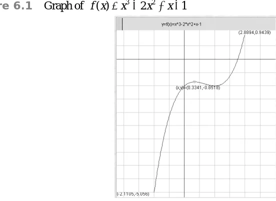
At this point we should be comfortable calculating the derivative of a given function which in turn tells us about the instantaneous rate of change of the given function. Now we want to reverse the process. That is, if we are given information about the first derivative of some function what can we find out about the original function? To investigate this, let’s look at the graph of f x( )=x3−2x2+ −x 1 shown in figure 6.1 below.
Figure 6.1 Graph of f x( )=x3−2x2+ −x 1
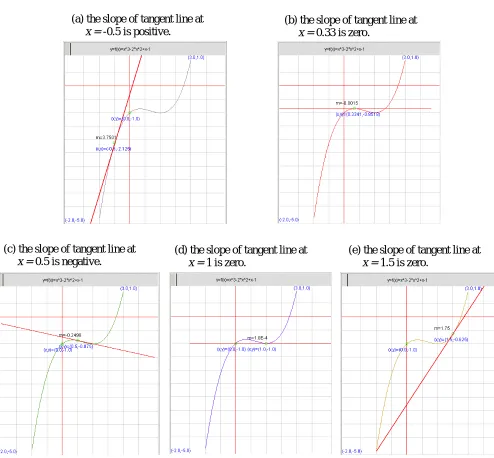
Figure 6.2 Graph of f x( )=x3−2x2+ −x 1 and tangent lines at various x values.
Notice that when the tangent line has a positive slope, the graph of f x( )=x3−2x2+ −x 1 is increasing as shown in figures (a) and (e) above. When the tangent line has a negative slope, the graph of
3 2
( ) 2 1
f x =x − x + −x is decreasing as shown in figure (c) above. Lastly, when the tangent line has a slope of zero, the graph of f x( )=x3−2x2+ −x 1 is neither increasing nor decreasing, we say the graph is constant, as shown in figures (b) and (d) above. Will this always be true? As it turns out this relationship between slopes of tangent lines and original functions will always be true. Consequently, we can conclude the following about a given function ( )f x and its first derivative f x'( ).
(a) the slope of tangent line at x = -0.5 is positive.
(b) the slope of tangent line at x = 0.33 is zero.
(c) the slope of tangent line at x = 0.5 is negative.
(d) the slope of tangent line at x = 1 is zero.
Increasing/Decreasing/Constant Intervals
Given a function, ( )f x , that is differentiable and continuous on an open interval ( , )a b 1) if f x'( )>0 for all x on ( , )a b , then ( )f x is increasing on ( , )a b .
2) if f x'( )<0 for all x on ( , )a b , then ( )f x is decreasing on ( , )a b . 3) if f x'( )=0 for all x on ( , )a b , then ( )f x is constant on ( , )a b .
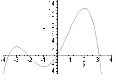
Example 6.1 Use the graph of ( )f x below to find the intervals where the function is increasing, decreasing, and constant.
When a function changes from increasing to decreasing at a critical value x = c, a relative (local)
maximum is formed. That is, at x = c, 𝑓𝑓(𝑥𝑥) <𝑓𝑓(𝑐𝑐) for all x in an open interval that contains c. When a function changes from decreasing to increasing at a critical value x = c, a relative (local) minimum is formed. That is, at x = c, 𝑓𝑓(𝑥𝑥) <𝑓𝑓(𝑐𝑐) for all x in an open interval that contains c. It is important to note here that the term relative (local) extrema is often used to refer to a relative (local) minimum, relative (local) maximum, or both. Figure 6.3 below shows an examples of relative (local) extrema at x = 3.
Figure 6.3
(a) a relative minimum exists at x = 3.
Relative minimum at x =3.
(b) a relative maximum exists at x = 3.
Once the critical value(s), also referred to as stationary points, have been found, we can then determine the intervals where the function increases and decreases. Critical values are found using the following definition.
Definition Critical Value (Stationary Points)
The value x = c is a critical value if the following two criteria are upheld. 1) f c'( )=0 or f c'( )does not exist and
2) x = c is in the domain of ( )f x
Example 6.2 Use the graph of ( )f x below and locate any the critical values.
Example 6.3 Find the critical values for f x( )=x3−2x2+ −x 1.
Example 6.4 Find the vertex of 𝑓𝑓(𝑥𝑥) =𝑥𝑥2−8𝑥𝑥+ 14.
Example 6.5 Find the stationary points of f and classify these points as a maximum or minimum for
𝑓𝑓
(𝑥𝑥
)= 2
𝑥𝑥
3+ 3
𝑥𝑥
2−
12
𝑥𝑥 −
4
.
2 2
Now that we know how to find critical values, we will further our analysis by finding the intervals where functions increase and decrease. To make this process as organized as possible, we will always construct a first derivative chart to help us perform the analysis. Suppose we want to find the intervals where
3 2
( ) 2 1
f x =x − x + −x increases and decreases. We found in example 6.3 that this function has critical values at 1
3
x= and x=1. To find the intervals where this function increases and decreases we first plot the critical values on a number line.
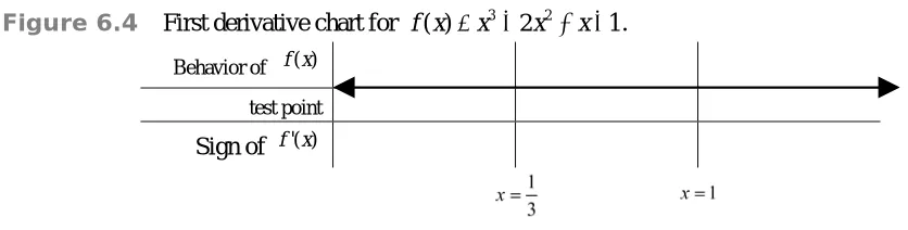
Figure 6.4 First derivative chart for f x( )=x3−2x2+ −x 1.
Behavior of f x( )
test point
Sign of f x'( )
To determine the behavior of f x( ) on these intervals, we need to determine the sign (whether it be positive or negative) of f x'( ) on these intervals. To do this, we must choose a test point for each interval, substitute this test point into 𝑓𝑓′(𝑥𝑥), and then record the sign of our answer. A test point is any number that lies on the interval.
Table 6.1 2
'( ) 3 4 1
f x = x − x+ evaluated at each chosen test point.
Test Point f'(test point) Sign of f'(test point)
Example 6.6 Find the intervals on which f x( )=x23 increases and decreases then find any relative extrema.
Example 6.9 A company has found that their revenue function, in thousands of dollars, is closely modeled by the function R x( )= −0.05x2+10x−350 for 0≤ ≤x 185 where x is the number of individual units sold. How many units must the company sell to maximize their revenue? What is the maximum revenue?
Example 6.10 The same company from example 6.9 has also determined that their cost function can be modeled by ( )C x =0.8x+20 where C x( ) is in thousands of dollars and x is the number of individual units sold. How many units must the company sell in order to maximize their profit? What is the company’s maximum profit?
6.2 The Second Derivative
Since the derivate of a function is a function itself it is possible to take its derivative. The derivative of the first derivative is called the second derivative and it is typically denote using a double prime, f''( )x . The second derivative of a function is a function itself and therefore has its own derivative. The derivative of the second derivative is called the third derivative and can be denoted with a triple prime,
'''( )
f x . We can continue this process and take numerous derivatives of functions; however, derivatives higher than the second do not serve any real purpose for our function analysis so we will stick to taking just the first and second derivative of a given function.
Example 6.11 Find the second derivative of f x( )= − +x3 4x2− −x 3.
Figure 6.11 The graph of f x( )= − +x3 4x2− −x 3 on 4 3
(−∞, ) and a table of values for f x'( ) is below.
If we look at the table of values we notice that the values of f x'( )are increasing as x approaches 1.3 from its left side and the graph of ( )f x is concave up.
Now let’s looks at the graph of f x( )= − +x3 4x2− −x 3 on 4 3
( , )∞ and some values for f x'( ) as shown in figure 6.12 below.
Figure 6.12 Graph of f x( )= − +x3 4x2− −x 3 on 4 3
( , )∞ and a table of values for f x'( ).
If we look at the table of values we notice that the values of f x'( ) are decreasing as x goes from 1.3 toward positive infinity and the graph of ( )f x is concave down. Thus, we see that
3 2
( ) 4 3
f x = − +x x − −x is concave up on 4 3
(−∞, )and concave down on 4 3
( , )∞ . Since the concavity changes and a tangent line exists at 4
3
x= , f x( ) has a point of inflection at
(
4 11) (
)
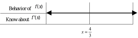
3, 27 ≈ 1.33, 0.41 . Figure 6.13 below organizes the information we acquired about f x( )= − +x3 4x2− −x 3 in the form of a chart.Figure 6.13 Chart displaying information about f x( )= − +x3 4x2− −x 3.
Behavior of ( )f x
Know about f x'( )
X -1.5 -1 -.5 0 .5 1 1.1 1.2 1.3
'( )
f x -19.75 -12 -5.75 -1 2.25 4 4.17 4.28 4.33
x 1.3 1.4 1.5 1.6 1.8 2 2.5 3 3.5
'( )
Recall that when a function is increasing the slopes of its tangent lines are all positive and when a function is decreasing the slopes of its tangent lines are all negative. Thus, when f x'( ) is increasing,
''( )
f x is positive and when f x'( ) is decreasing, f''( )x is negative. If we add this information to the chart from figure 6.13 we obtain a chart as shown in figure 6.14 below.
Figure 6.14 Chart displaying information about f x( )= − +x3 4x2− −x 3.
Behavior of f x( )
Know about f x'( )
Sign of f''( )x
We can see from the figure 6.14 that when the second derivative is positive ( f''( )x >0) the graph ( )f x is concave up and when the second derivative is negative (f''( )x <0) the graph of ( )f x is concave down. When the second derivative is zero ( f''( )x =0) the graph of ( )f x has a point of inflection. The
conclusions about the second derivative of a function are stated below.
Intervals of Concavity and Points of Inflection
Given a function ( )f x that is twice differentiable and continuous on an open interval ( , )a b
• if f''( )x >0 for all x on ( , )a b , then ( )f x is concave up on ( , )a b . • if f''( )x <0 for all x on ( , )a b , then ( )f x is concave down on ( , )a b .
• if f''( )x =0 or f''( )x does not exist, a point of infection exists at
(
x f x, ( ))
provided ( )f x changes concavity and a tangent line exists at(
x f x, ( ))
,Recall from the example above the value 4 3 x=
was the value at which concavity changed and thus
(
4 11) (
)
3, 27 ≈ 1.33, 0.41 was a point of inflection. Use the definition of point of inflection from above we can now show the calculation used to find the point of inflection.
2
'( ) 3 8 1
f x = − x + x− so f''( )x = − +6x 8
0 6 8
Example 6.12 Given ( )f x below, find the intervals where it is concave up and concave down then determine all points of inflection.
4 3 2
1 1
( )
12 6
f x = x + x −x
6.4 Function Analysis using Derivatives
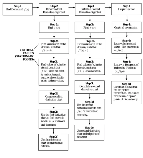
At this point you may be feeling a bit overwhelmed with all the information concerning function analysis using the first and second derivatives. Let’s try to ease your pain by organizing this information in the form of a flow chart as shown in the flow chart below in figure 6.4a
“FUN” Chart:
Figure 6.4a Flow chart for function analysis.
Step 1 Find Domain of
Step 2 Perform a First Derivative Sign Test
Step 3 Perform a Second Derivative Sign Test
Step 4 Graph Function
Step 2b Find values of x, in the domain, such that
.
Step 2c Find values of x, in the domain, such that
does not exist. A vertical tangent, cusp, or discontinuity exists at these values.
Step 2d Complete a first derivative chart
Step 2e Use the first derivative chart to find intervals where increases and decreases.
Step 2f Use first derivative chart to find relative extrema. CRITICAL VALUES (STATIONARY POINTS) Step 3b Find values of x, in the domain, such that
.
Step 3c Find values of x, in the domain, such that
does not exist.
Step 3c Complete a second
derivative chart
Step 3d Use the second derivative chart to find
’s intervals of concavity.
Step 3e Use second derivative chart to find points of inflection.
Step 4b Let x =c be a critical value. Plot extrema at
. Step 4a Graph all asymptotes.
Step 4d Construct a curve that fits the plotted information. Be sure to include any cusps or points of discontinuity.
Step 4c Let x = p be a point of inflection. Plot it at
. Step 2a
Find
Example 6.4b Given f x( )=x13 find the intervals where ( )f x increases and decreases, all relative extrema, the intervals where ( )f x is concave up and down, and all points of inflection. Then construct a graph of ( ).f x
Example 6.4c Given f x'( )=(x−2)3 and the domain of ( )f x is (−∞ ∞, ), find the intervals where ( )
f x increases and decreases, all relative extrema, intervals where ( )f x maybe concave up or down. Then sketch a possible graph of f(x).
Example 6.4d Sketch a graph of a function that fulfils the following criteria. • Domain (−∞, 4)and Range (−∞,3)
• f x'( )>0 on (−∞ − ∪, 2) (0, 2) and f x'( )<0 on ( 2, 0)− ∪(2, 4) • f x'( )=0 at x= −2 and x=2 and f x'( ) does not exist at x=0 • f''( )x <0 on (−∞, 0)∪(0, 4)
• ( 2)f − =3, f(0)=0, f(2)=2, f(4)= −1
Example 6.4e Given the graph of f x'( ) below, sketch a possible graph of ( )f x that is everywhere continuous and has a domain and range of (−∞ ∞, ).
2 4 6
2 4 6
–2 –2 –4