www.biogeosciences.net/bg/3/29/ SRef-ID: 1726-4189/bg/2006-3-29 European Geosciences Union
Biogeosciences
DMS cycle in the marine ocean-atmosphere system – a global model
study
S. Kloster, J. Feichter, E. Maier-Reimer, K. D. Six, P. Stier, and P. Wetzel
Max Planck Institute for Meteorology, Hamburg, Germany
Received: 22 July 2005 – Published in Biogeosciences Discussions: 22 August 2005 Revised: 11 November 2005 – Accepted: 9 December 2005 – Published: 11 January 2006
Abstract. A global coupled ocean-atmosphere modeling system is established to study the production of dimethyl-sulfide (DMS) in the ocean, the DMS flux to the sphere, and the resulting sulfur concentrations in the atmo-sphere. The DMS production and consumption processes in the ocean are simulated in the marine biogeochemistry model HAMOCC5, embedded in a ocean general circula-tion model (MPI-OM). The atmospheric model ECHAM5 is extended by the microphysical aerosol model HAM, treat-ing the sulfur chemistry in the atmosphere and the evolution of the microphysically interacting internally- and externally mixed aerosol populations.
We simulate a global annual mean DMS sea surface con-centration of 1.8 nmol l−1, a DMS emission of 28 Tg(S) yr−1, a DMS burden in the atmosphere of 0.077 Tg(S), and a DMS lifetime of 1.0 days. To quantify the role of DMS in the atmo-spheric sulfur cycle we simulate the relative contribution of DMS-derived SO2and SO24−to the total atmospheric sulfur concentrations. DMS contributes 25% to the global annually averaged SO2column burden. For SO24−the contribution is 27%.
The coupled model setup allows the evaluation of the sim-ulated DMS quantities with measurements taken in the ocean and in the atmosphere. The simulated global distribution of DMS sea surface concentrations compares reasonably well with measurements. The comparison to SO24− surface con-centration measurements in regions with a high DMS contri-bution to SO24−shows an overestimation by the model. This overestimation is most pronounced in the biologically active season with high DMS emissions and most likely caused by a too high simulated SO24−yield from DMS oxidation.
Correspondence to: S. Kloster
(kloster@dkrz.de)
1 Introduction
Major uncertainties remain in the quantitative assessment of the climate response to anthropogenic forcing. Biogeochem-ical feedbacks, which may reduce or amplify the net impact of the anthropogenic forcing, are extremely important to the understanding and prediction of climate change (Lovelock et al., 1972). One possible negative biogeochemical feed-back proposed by Charlson et al. (1987) involves the marine biosphere, the ocean and the atmosphere coupled through the marine biogenic sulfur compound dimethylsulfide (DMS).
DMS produced from phytoplankton is the most abundant form in which the ocean releases gaseous sulfur. In the at-mosphere, DMS is oxidized to sulfate particles that alter the amount of solar radiation reaching the Earth’s surface both by directly scattering solar energy and indirectly by acting as cloud condensation nuclei (CCN), thereby affecting the cloud albedo. The change in cloud albedo results in global temperature perturbations potentially affecting the produc-tivity of the marine biosphere and hence the concentration of oceanic DMS. The oceanic and atmospheric processes in-volved in this multistep feedback mechanism are complex. Fundamental gaps remain in our understanding of key is-sues in this feedback process, in particular with regard to the processes that regulate the DMS seawater concentration (Andreae and Crutzen, 1997; Liss et al., 1997; Gabric et al., 2001; V´ezina, 2004). Traditionally, the DMS cycle in the atmosphere and in the ocean have been assessed indepen-dently. As a consequence, it has not been possible to assess the strength of the proposed feedback or even to anticipate if global warming will result in an increase or a decrease of DMS emissions. However, significant progress has been made to understand many of the included mechanisms.
and especially of its degradation to DMS, is still not clear. It has been suggested that the physiological function of DMSP is related to maintaining intercellular osmotic pres-sure (Vairavamurthy et al., 1985). Other suggested physio-logical functions of DMSP in marine algae are that it may act as a cryoprotectant (Kirst et al., 1991; Stefels, 2000) and serve as an antioxidant system (Suda et al., 2002).
DMSP is widespread among taxa but seems to be par-ticularly abundant in specific groups, including coccol-ithophorids like Emiliania huxleyi. Other groups, like di-atoms, are generally poor producers of DMSP (Keller et al., 1989). Among other factors, DMSP release into the water is assumed to be controlled by phytoplankton senescence (Nguyen et al., 1990; Kwint and Kramer, 1995), viral lysis of phytoplankton cells (Malin et al., 1998) and zooplankton grazing (Dacey and Wakeham, 1986). Dissolved DMSP is degraded to DMS via enzymatic cleavage carried out by al-gal or bacterial DMSP lyase (Steinke et al., 2002; Yoch et al., 1997). A large fraction of DMSP is utilized by bacteria and does not lead to the production of DMS (Kiene, 1996). Kiene et al. (2000) hypothesized that the sulfur-demand of bacte-ria determines the proportion on which DMSP is processed through this demethylation pathway, rather than being con-verted by enzymatic degradation to DMS.
Consumption by bacteria is the major sink for DMS in sea-water (Kiene and Bates, 1990; Dacey and Wakeham, 1986). Chemical oxidation of DMS to dimethyl sulfoxide (DMSO) in seawater and ventilation to the atmosphere contribute only a minor part to the total DMS removal in seawater (e.g. Shooter and Brimblecombe, 1989; Kieber et al., 1996; Bates et al., 1994; Gabric et al., 1993).
DMS sea-air fluxes may vary by orders of magnitude in space and time. Although there are no direct means of mea-suring DMS sea-air flux, it can be estimated from the DMS sea surface concentration combined with an empirically de-termined exchange rate. Parameterization of DMS sea-air exchange rates have been investigated in several studies (e.g. Wanninkhof, 1992; Wanninkhof and McGillis, 1999; Liss and Merlivat, 1986; Nightingale et al., 2000; McGillis et al., 2000; Zemmelink et al., 2002). According to Nightingale et al. (2000), the uncertainties associated with the exchange rate are approximately 50%.
Many aspects of the DMS oxidation in the atmosphere are poorly understood (e.g. Campolongo et al., 1999; Andreae and Crutzen, 1997). It is well-established that OH reacts with DMS and that SO2 and methane sulfonic acid (MSA) are among the major reaction products (e.g. Capaldo and Pandis, 1997). It is also known that NO3and halogen oxide radicals (e.g. BrO, IO, ClO) react with DMS in the atmosphere, but the importance of these reactions is even less well-known (Sayin and McKee, 2004).
A key link in the proposed feedback between DMS and climate is the nucleation of DMS-derived sulfuric acid into new particles and eventually the formation of new cloud-forming particles (Charlson et al., 1987). The nucleation
ability of DMS-derived sulfuric acid in the marine boundary layer is still under debate (Yoon and Brimblecombe, 2002). Measurements over the South Atlantic, at Cape Grim, and at Amsterdam Island show a strong correlation between DMS emission and the concentration of total aerosol particles and CCN (Putaud et al., 1993; Andreae et al., 1995, 1999; Ayers and Gillett, 2000). However, such findings are by no means generally applicable. Several investigators found no or only sporadic correlation between DMS and non-sea-salt sulfate, CN or CCN (Bates et al., 1992; Berresheim et al., 1993).
DMS and its oxidation products in the atmosphere are short-lived species. Therefore, it is necessary to resolve the temporal and spatial distribution of the DMS sea surface con-centration on a global scale to investigate its impact on the climate system. Several studies attempted to build clima-tologies of the global distribution of DMS in the sea sur-face water. Belviso et al. (2004a) recently compared seven global DMS monthly climatologies (Kettle et al., 1999; Ket-tle and Andreae, 2000; Anderson et al., 2001; Aumont et al., 2002; Sim´o and Dachs, 2002; Chu et al., 2003; Belviso et al., 2004b). For the zonal and annual mean they found differ-ences ranging from 50% in the tropics to 100% in high lat-itudes. The studies of Kettle et al. (1999); Kettle and An-dreae (2000); Anderson et al. (2001); Sim´o and Dachs (2002) all rely on the Kettle et al. (1999) database which consists of almost 16 000 DMS sea surface measurements. Kettle et al. (1999) and Kettle and Andreae (2000) derived monthly mean maps by a compilation of the measurements included in the database. Anderson et al. (2001) and Sim´o and Dachs (2002) used only the data points from the Kettle et al. (1999) database with concurrent chlorophyllα and DMS sea sur-face measurements and extended the resulting database by climatological information about incoming light and nutri-ent abundance or by information about the mixed layer depth (MLD), respectively. From the extended database they de-rived nonlinear relationships to predict DMS sea surface con-centrations. Aumont et al. (2002) and Belviso et al. (2004b) used a prognostic nonlinear parameterization to compute DMS sea surface concentrations from chlorophyllα concen-trations together with an index of community structure of marine phytoplankton derived from measurements taken at several DMS surveys. Only the approach of Chu et al. (2003) uses a prognostic biogeochemical formulation for DMS pro-duction and DMS removal in the ocean based on the regional work of Gabric et al. (1993).
rate which varies with wind speed and temperature. Pen-ner et al. (2001) showed a small increase in simulated DMS emissions between 2000 and 2100 (from 26.0 Tg(S)yr−1to 27.7 Tg(S)yr−1) using a constant DMS sea surface concen-tration field (Kettle et al., 1999) combined with a constant monthly climatological ice cover. The gas exchange rates were calculated interactively in the simulation based on wind speed and sea surface temperature. However, DMS sea sur-face concentrations are controlled by marine biology which is affected by climate variables such as solar radiation, tem-perature and ocean physics. These variables are likely to change under changing climate conditions.
Changes in climate will lead to changes in the emission of other components that are linked to the DMS cycle, e.g. sea salt aerosols (Gong and Barrie, 2003), emissions associated with organic aerosols (O’Dowd et al., 1999) and dust emis-sions (Tegen et al., 2004). Stier et al. (2004) showed in a global microphysical aerosol modeling study that specific emission changes cause changes in aerosol cycles of other components confirming a microphysical coupling between the different aerosol cycles. To account for these effects, the DMS-climate feedback has to be studied as a part of the com-plex global aerosol system.
To assess the role of DMS in the climate system, it is essential to treat the DMS cycle interactively in the ocean-atmosphere system, as the proposed DMS-climate feedback is a multi-compartment feedback. This requires a coupled ocean-atmosphere model with prognostic treatment of the marine DMS and the atmospheric sulfur cycle. This study introduces such a comprehensive model, describes the simu-lated multi-compartment sulfur cycle and provides an evalu-ation with available measurements. Additionally, simulated DMS sea surface concentrations are compared to DMS con-centrations derived with the recently developed Sim´o and Dachs (2002) algorithm. Particular attention is given to the implementation of a formulation of DMS production and degradation in the ocean in order to simulate dynamically consistent maps of DMS sea surface concentrations, which provides the basis for an assessment of interactions between marine DMS and the atmosphere.
2 Model description
The model used in the experiment is a coupled atmosphere-ocean general circulation model (AOGCM). The AOGCM consists of sub-models which correspond to the atmosphere (ECHAM5) and the ocean (MPI-OM). The atmospheric model includes a microphysical aerosol model (HAM) which simulates the evolution of an ensemble of microphysically interacting internally- and externally mixed aerosol popu-lations as well as their size-distribution and composition. Embedded in the ocean model is a marine biogeochemistry model (HAMOCC5) which has been extended by a
formula-tion of the DMS cycle in the ocean. The single model com-ponents are briefly described in the following sections. 2.1 The MPI-OM general circulation model
The ocean component is the Max-Planck-Institute ocean model (MPI-OM) (Marsland et al., 2003). MPI-OM is a z-coordinate global general circulation model based on the primitive equations for a Boussinesq-fluid on a rotating sphere. The transport is computed with a total variation di-minishing (TVD) scheme (Sweby, 1984). It includes param-eterizations of sub grid scale mixing processes like isopyc-nal diffusion of the thermohaline fields, eddy induced tracer transport following Gent et al. (1995), and a bottom bound-ary slope convection scheme. The model treats a free sur-face and a state of the art sea ice model with viscous-plastic rheology and snow (Hibler, 1979). The model works on a curvilinear orthogonal C-grid. In this study, we use a nom-inal resolution of 1.5◦at the equator with one pole located
over Greenland and the other over Antarctica. In the verti-cal, the model has 40 levels with level thickness increasing with depth. 8 layers are located within the upper 90 m and 20 layers within the upper 600 m.
2.2 The marine biogeochemistry model HAMOCC5 The marine biogeochemistry component is the Hamburg Oceanic Carbon Cycle Model (HAMOCC5) (Maier-Reimer et al., 2005; Six and Maier-Reimer, 1996; Maier-Reimer, 1993). HAMOCC5 simulates the biogeochemical tracers in the oceanic water column and the sediment. The model is coupled online to the circulation and diffusion of the MPI-OM ocean model and runs with the same time step and resolution. The eco-system model is based on nutri-ents, phytoplankton, zooplankton and detritus (NPZD-type) as described in Six and Maier-Reimer (1996). In addition, new elements like nitrogen, dissolved iron and dust are ac-counted for and new processes like denitrification, nitrogen fixation, dissolved iron uptake and release by biogenic par-ticles, and dust deposition and sinking are implemented as described in detail in Wetzel (2004). The dust deposition to the ocean surface is calculated online in the ECHAM5-HAM submodel and passed to the marine biogeochemistry model HAMOCC5 once per day. Bioavailable iron is released in the surface layer immediately from the freshly deposited dust. 2.2.1 DMS formulation in the marine biogeochemistry
module HAMOCC5
The DMS formulation in HAMOCC5 is derived from the for-mulation originally developed for a former version of the ma-rine biogeochemistry module (HAMOCC3.1, Six and Maier-Reimer, 1996; Six and Maier-Maier-Reimer, 20061).
Bio-Table 1. Parameters for DMS formulation in HAMOCC5. The
pa-rameters are derived from an optimization procedure of HAMOCC5 using DMS sea surface concentration measurements from the Kettle and Andreae (2000) database.
Symbol constant Process
DMS Production
kpsi 0.0136 (S(DMS)/(Si)) silicate kpcc 0.1345 (S(DMS)/(C)) calcium
carbonate
kpt 10.01 (◦C) temperature
dependence
DMS Decay
kluv 0.0011 (m2(W d)−1) photolysis klb 0.1728 (d−1◦C−1) bacteria
The formulation for DMS production in the ocean assumes that DMS is produced (DMSprod) when phytoplankton cells are destroyed due to senescence or grazing processes. The DMS decay occurs via consumption by bacteria (DMSbac), chemical oxidation to DMSO (DMSUV) and ventilation to the atmosphere (DMSflux).
d[DMS]
dt =DMSprod−DMSbac−DMSUV−DMSflux (1) Here only dissolved DMS is considered. DMSP as the pre-cursor of DMS in the ocean is not taken into account explic-itly because very little is known about the actual processes that lead to the reduction of DMSP to DMS (Kiene et al., 2000). Moreover, only few measurements of DMSP concen-trations in the ocean are available which makes an evaluation not feasible.
HAMOCC5 was developed to simulate the carbon chem-istry in the ocean. To simulate the vertical alkalinity distribu-tion it separates between the export of particulate silicate and calcium carbonate (exportsilandexportCaCO3, respectively).
The resulting vertical alkalinity distribution compares well with available measurements (Wetzel et al., 2005; Wetzel, 2004). By separating the export into the export of cal-cium carbonate and the export of silicate, HAMOCC5 distin-guishes indirectly between the two phytoplankton groups the diatoms which form opal frustels, and the coccolithophorids which build skeletons made of calcium carbonate. It is as-sumed that fast growing diatoms consume nutrients as long as silicate is available. Therefore, the export of organic car-bon is linked to silicate until silicate is depleted in the ocean. After depletion of silicate the phytoplankton growth is car-ried out by coccolithophorids, resulting in the export of cal-cium carbonate. The simulated ratio of calcal-cium carbonate geochem. Cycles, submitted, 2006.
to organic carbon export is tuned to be 0.06 on global av-erage in order to simulate a realistic alkalinity distribution (Wetzel, 2004; Sarmiento et al., 2002). This distinction be-tween diatoms and coccolithophorids is important, as they are known to differ markedly in terms of their cellular DMSP content, and hence their ability for producing DMS (Keller et al., 1989). We utilize the distinction between silicate and calcium carbonate export to simulate the DMS production as follows:
DMSprod=f (T )×(kpsi×exportsil+kpcc×exportCaCO3)(2)
kpsiandkpccare the respective scaling factors defined in
Ta-ble 1. The function f (T )accounts for the observed tem-perature dependence of intercellular DMSP concentrations. Under low temperature conditions, e.g. in polar regions, the DMSP content in phytoplankton cells is higher than under temperate conditions (Baumann et al., 1994). This effect is parameterized as follows:
f (T )=
1+ 1
(T +kpt)2
(3) withT in◦C,kpt scales the temperature dependency
(Ta-ble 1).
The DMS destruction processes are formulated as follows: The destruction of DMS by photo-oxidation to DMSO de-pends on the solar radiation at the surface (Shooter and Brim-blecombe, 1989; Brimblecombe and Shooter, 1986; Kieber et al., 1996). The incident solar radiation I0 is attenuated in HAMOCC5 by water and phytoplankton as a function of depth (z) according to the equation:
Iz=I0×e−(kw+kchl)×z (4)
The attenuation coefficient for pure water is chosen to be kw=0.04 m−1. Light attenuation by phytoplankton is
as-sumed to be a linear function of the chlorophyll concentra-tionkchl=0.03[CHL]m−1, with the chlorophyll concentra-tion[CHL]given in mg l−1. The chlorophyll concentration is computed from the modeled phytoplankton concentration with a fixed chlorophyll to carbon ratio of 1:60. The incident surface radiation(W m−2)is calculated interactively, includ-ing the effects of clouds and aerosols, in the ECHAM5-HAM model. The decay of DMS by photo-oxidation is then formu-lated as follows:
DMSUV=kluv×Iz× [DMS] (5)
kluvis the respective scaling factor defined in Table 1. DMS destruction due to consumption by bacteria is assumed to be temperature dependent:
DMSbac=klb×(T +3.)× [DMS] ×f ([DMS]) (6)
withT in◦C.klbdenotes the scaling factor for the
[image:4.595.45.296.132.266.2]DMS concentrations (Kiene and Bates, 1990). We parame-terize this variation with a saturation function:
f ([DMS])=
[DMS]
kcb+ [DMS]
(7) kcbis set to 10 nmol l−1which ensures an almost linear
be-havior for low DMS concentrations. For the atmosphere, the most important DMS loss mechanism in seawater is the loss due to sea-air exchange. For the sea-air exchange calculation we neglect the DMS concentration in the atmosphere, as it is small compared to the DMS sea surface concentration, and formulate the DMS sea-air exchange as:
DMSflux=ksea−air× [DMS] (8)
ksea−air denotes the sea-air exchange rate. We choose the formulation after Wanninkhof (1992):
ksea−air=0.31×w210 m×
SC
660
−12
(9) wherew10is the 10 m wind speed andSCthe Schmidt num-ber for DMS which is calculated analogous to Saltzman et al. (1993).
The undetermined parameters are derived from a fit of the simulated DMS sea surface concentrations to observed DMS sea surface concentrations. Kettle and Andreae (2000) com-piled a database of almost 16 000 DMS sea surface concen-tration measurements. Thereby, the original database (Kettle et al., 1999) was updated by new measurements. We utilized the updated database for an optimization of the parameters in the proposed DMS formulation. Therefore, the data points are distributed onto the ocean grid cells on a monthly mean basis. The DMS grid value is taken to be the average of the individual monthly mean measurements within the grid cell. Since the data coverage is very sparse and the partitioning into monthly means is rather arbitrary, we extrapolated the resulting DMS sea surface concentration for a single grid box to the adjacent grid boxes and also took values from the adjacent months into account for the monthly splitting. Due to computational constraints it is not feasible to conduct the optimization process within the full coupled AOGCM. To derive the DMS scaling parameters, we use an offline version of the ocean model (MPI-OM/HAMOCC5) forced by NCEP/NCAR reanalysis data (Kalnay et al., 1996). The model setup is described in detail in Wetzel et al. (2005). From this simulation we arbitrarily choose the year 1995 for the optimization process of the DMS scaling parameters. Pe-riodically repeating the simulation with NCEP/NCAR forc-ing fields for the year 1995, we calculate global value devi-ation fields of the modeled DMS sea surface concentrdevi-ation and the DMS sea surface map, generated from the Kettle and Andreae (2000) database. Thereby, we take only ocean grid boxes into account with an ocean depth greater than 300 m. Regions with a shallower depth, like the North Sea, are not well captured by the model. In these regions the Kettle
and Andreae (2000) database includes a disproportional high number of measurements. To avoid a bias in the optimiza-tion process towards these measurements, these grid boxes are excluded. We define a cost function as the global an-nual sum of the deviation fields. In a series of two year runs, starting with the same initial conditions, this cost function is minimized by changing the five free parameters (kpsi,kpcc,
kpt,kluv,klb) of the DMS formulation sequentially by plus or
minus 5%. The cost function is then calculated during every second model year. The parameters are changed along the gradient leading to a minimum of the cost function. The task of this global optimization process is to find the global min-imum of the cost function. However, we cannot exclude that this optimization process leads to a local minimum, which is a general problem in optimization procedures. The resulting parameters of the optimization parameters are compiled in Table 1.
2.3 The ECHAM5 general circulation model
The atmospheric component is the ECHAM5 model (Roeck-ner et al., 2003) with the current standard resolution of 31 vertical levels on a hybrid sigma-pressure coordinate sys-tem up to a pressure level of 10 hPa. Prognostic variables are vorticity, divergence, surface pressure, temperature, wa-ter vapor, cloud wawa-ter and cloud ice. Except for the wawa-ter and chemical components, the prognostic variables are rep-resented by spherical harmonics with triangular truncation at wavenumber 63 (T63). Physical processes and nonlinear terms are calculated on a Gaussian grid with a nominal res-olution of 1.8◦in longitude and latitude. For the advection
of water vapor, cloud liquid water, cloud ice and tracer com-ponents, a flux form semi-Lagrangian transport scheme (Lin and Rood, 1996) is applied. Cumulus convection is based on the mass flux scheme after Tiedtke (1989) with modifica-tions according to Nordeng (1994). The cloud microphysi-cal scheme (Lohmann and Roeckner, 1996) consists of prog-nostic equations for cloud liquid water and cloud ice. The cloud cover is predicted with a statistical scheme including prognostic equations for the distribution moments (Tomp-kins, 2002). The transfer of solar radiation is parameterized after Fouquart and Bonnel (1980) and the transfer of long-wave radiation after Morcrette et al. (1998).
2.4 The HAM aerosol model
Table 2. Aerosol and aerosol precursor emissions used in the HAM model. Global annual mean in Tg yr−1and Tg(S)yr−1for sulfuric species.
Species Source Reference Tg yr−1
DMS Terrestial Biosphere Pham et al. (1995) 0.3
Marine Biosphere HAMOCC5 27.6
SO2 Volcanoes Andres and Kasgnoc (1998) 14.6 Halmer et al. (2002)
Vegetation Fires van der Werf et al. (2003) 2.1 Industry, Fossil-Fuel, Cofala et al. (2005) 54.2 Bio-Fuels
Total sulfur 99.0
BC Vegetation Fires van der Werf et al. (2003) 3.0 Fossil-Fuel and Bond et al. (2004) 4.7 Bio-Fuels
Total BC 7.7
POM Vegetation Fires van der Werf et al. (2003) 34.7 Biogenic Guenther et al. (1995) 19.1 Fossil-Fuel and Bond et al. (2004) 12.5 Bio-Fuels
Total POM 66.3
SSA Wind driven Schulz et al. (2004) 5868.6
DU Wind driven Tegen et al. (2002) 1060.6
compounds, four of the modes contain at least one soluble compound. Aerosol compounds considered are sulfate (SU), black carbon (BC), particulate organic mass (POM), sea salt (SSA), and mineral dust (DU). HAM consists of a micro-physical core M7, an emission module, a sulfur chemistry scheme, a deposition module, and a radiation module defin-ing the aerosol radiative properties.
The microphysical core M7 (Vignati et al., 2004) treats the aerosol dynamics and thermodynamics. Processes con-sidered are coagulation among the modes, condensation of gas-phase sulfuric acid on the aerosol surface, the binary nu-cleation of sulfate, and water uptake.
The emission of mineral dust and sea salt is calculated in-teractively according to the scheme of Tegen et al. (2002) and Schulz et al. (2004), respectively. DMS emissions are calculated online in the marine biosphere submodel HAMOCC5. For the other aerosol compounds, emission strengths, emission size distribution and emission height are based on the AEROCOM (Aerosol Model Inter-Comparison, http://nansen.ipsl.jussieu.fr/AEROCOM) emission inventory for the year 2000 (Dentener et al., 20062). The emission 2Dentener, F., Kinne, S., Bond, T., Boucher, O., Cofala, J., Gen-eroso, S., Ginoux, P., Gong, S., Hoelzemann, J. J., Ito, A., Marelli, L., Penner, J., Putaud, J.-P., Textor, C., Schulz, M., van der Werf, G., and Wilson, J.: Emissions of primary aerosol and aerosol
pre-strength for all aerosol compounds is summarized in Table 2. The sulfur chemistry module (Feichter et al., 1996) treats DMS, SO2 and SO24− as prognostic variables. In the gas phase, SO2 and DMS are oxidized by hydroxyl (OH) dur-ing the day. Additionally, DMS reacts with nitrate radicals (NO3) at night. Reaction products are SO2and SO24−. Dis-solution of SO2 within cloud water is calculated according to Henry’s law. In the aqueous phase, the oxidation of SO2 by hydrogen peroxide (H2O2) and ozone (O3) are consid-ered. The oxidant concentrations are prescribed as three dimensional monthly mean fields from calculations of the MOZART chemical transport model (Horowitz et al., 2003). Gas phase produced sulfate is allowed to condensate onto pre-existing particles or to nucleate to new particles, calcu-lated by the aerosol microphysical module M7. In-cloud pro-duced sulfate is distributed to the available pre-existing ac-cumulation mode and coarse mode aerosol particles accord-ing to their respective number concentration. The deposition processes, i.e. wet deposition, dry deposition, and sedimenta-tion, are calculated online in dependence of aerosol size and composition.
sition and mixing state which are then passed to the radiation scheme of ECHAM5. Only the effects of the aerosols on the solar part of the spectrum are considered.
For this study the ECHAM5-HAM model has been ex-tended by a technique to mark SO2 and SO24− attributable to DMS. This allows to isolate the fraction of DMS-derived SO2 and SO24−. Such a quantification facilitates to assess the importance of aerosols of DMS origin. Additionally, the knowledge of the contribution of DMS to SO24−enables us to use SO24− concentration measurements at sites with a relatively high contribution of DMS to SO24−for an evalua-tion of the atmospheric DMS cycle in the model.
2.5 Model setup
The ocean and the atmosphere models are coupled with the OASIS coupler (Valcke et al., 2003) with a coupling time step of one day. The ocean model MPI-OM passes the sea surface temperature and sea ice variables to the atmosphere through OASIS. The atmosphere model ECHAM5-HAM uses these boundary conditions for one coupling timestep and transfers the surface forcing fields through OASIS back to the ocean model. Required surface forcing fields are heat, freshwa-ter and momentum fluxes, downward solar radiation and the 10 m wind speed. Additionally the DMS flux to the atmo-sphere calculated in HAMOCC5 is passed to the atmoatmo-sphere model and the dust deposition calculated in the HAM model is passed to HAMOCC5 through OASIS. The model does not employ flux adjustments.
In order to initialize the coupled atmosphere-ocean AOGCM, the uncoupled ocean model was integrated over thousand years to reach quasi-equilibrium state. From there on the coupled AOGCM was integrated with fixed external forcing to reach quasi-equilibrium state. From these ini-tial conditions the simulation is started and integrated for 15 years. The results presented here are averaged over the last 10 years.
3 Results
3.1 Ocean
A detailed description of the simulated ocean and biochem-ical mean state of MPI-OM/HAMOCC5 is given in Wetzel (2004). On average, the simulated global net primary pro-duction is 24 GtC yr−1. The export production, defined as the part of the net primary production that is transported out of the euphotic zone, amounts to 5 GtC yr−1, which is on the low end of model and observational estimates (Oschlies, 2002). The global annual averaged export of calcium car-bonate is 0.27 GtC yr−1, which leads to a rain ratio (the ratio of calcium carbonate to organic carbon in export production) of 0.06 on average. This ratio lies within current estimates
(Sarmiento et al., 2002) and leads to a realistic alkalinity dis-tribution.
Wetzel (2004) shows that the model is able to reproduce chlorophyll distribution from the SeaWIFS satellite, except for the coastal regions, where shelf processes and riverine in-put of nutrients are not captured by the global model. Ad-ditionally, the model tends to simulate higher chlorophyll concentrations in the Southern Ocean and in the subtropi-cal gyres than derived from satellite observations. Wetzel (2004) concludes that this might be predominantly a result of the modeled ocean dynamic with too strong vertical mix-ing in the Southern Ocean and a too weak downwellmix-ing in the subtropical gyres.
A novel feature of the coupled model used in this study, is that dust deposition fields are calculated interactively in the atmospheric model and passed once per day to the ocean, instead of prescribing the dust deposition from cli-matological mean fields. This provides the means to ap-ply this model for longterm climate change simulations including the effects of varying dust depositions, caused by climate change, on the marine biogeochemistry and on the DMS sea surface concentration. Assuming an iron content in dust of 3.5% we simulated an annual global mean iron deposition flux of 666 Gmol(Fe)yr−1, whereby 204 Gmol(Fe)yr−1are deposited to the ocean surface. The iron deposition onto the ocean surface lies within the range used in other global marine biogeochemistry studies (Fung et al., 2000: 118 Gmol(Fe)yr−1, Aumont et al., 2003: 149.7 Gmol(Fe)yr−1, Archer and Johnson, 2000: 131.7– 487.4 Gmol(Fe)yr−1). The wide range given in the global iron deposition rates highlights the uncertainties in the iron content of dust particles, as in the magnitude and the size variation of the dust emission and deposition in the atmo-sphere.
In the following section we will focus on the simulated DMS sea surface concentrations and compare our results to measurements as well as to a recently developed DMS algo-rithm by Sim´o and Dachs (2002).
3.1.1 DMS in the ocean
HAMOCC5 simulates a global total DMS production of 351 Tg(S)yr−1. The loss of DMS in the ocean proceeds mainly via the consumption by bacteria (294 Tg(S)yr−1). The DMS flux into the atmosphere (28 Tg(S)yr−1) accounts for 8% of the global DMS removal in the ocean, the photo-oxidation (31 Tg(S)yr−1) for 9%.
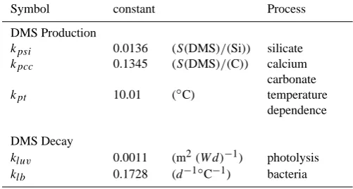
(a) (b)
[image:8.595.55.540.55.389.2](c) (d)
Fig. 1. Modeled seasonal mean DMS sea surface concentration. (a) Mean for December, January, February; (b) Mean for March, April,
May; (c) Mean for June, July, August; (d) Mean for September, November, December. Overlayed grid boxes are ocean data points given in the Kettle and Andreae (2000) database (data points where the ocean depth is below 300 m are excluded) gridded onto the model grid. Units are nmol l−1.
Tropical Pacific where measurements show a 3 to 430 times faster removal of DMS by biological consumption than by the DMS flux into the atmosphere (Kiene and Bates, 1990) and for the North East Pacific where biological consumption accounted for 67% of the total DMS consumption and the DMS flux accounted for only a small fraction (1%) of the DMS loss (Bates et al., 1994). The simulated annual mean decay rates are in accordance with these findings. However, for an evaluation of the simulated production and decay pro-cesses more measurements are needed.
The simulated seasonal mean sea surface concentrations of DMS are shown in Fig. 1. The predicted DMS con-centrations show moderate values, generally exceeding 1– 2 nmol l−1, in the biological active upwelling zones like the equatorial Pacific Ocean, or in the upwellings off Peru and Angola throughout the year. The subtropical gyres in both hemispheres show low DMS sea surface concentrations. The polar oceans (North Pacific, North Atlantic and Southern Ocean) feature high DMS concentrations with values up to 20 nmol l−1in the Southern Ocean in the respective summer seasons.
The predicted annual global mean DMS sea surface con-centration lies with 1.8 nmol l−1within the range of annual mean concentrations from DMS climatologies (Kettle et al., 1999: 2.1 nmol l−1, Kettle and Andreae, 2000: 2.0 nmol l−1, Anderson et al., 2001: 2.6 nmol l−1, Aumont et al., 2002: 1.7 nmol l−1, Sim´o and Dachs, 2002: 2.3 nmol l−1, Chu et al., 2003: 1.5 nmol l−1, Belviso et al., 2004b: 1.6 nmol l−1; global numbers taken from Belviso et al., 2004a).
a b
Fig. 2. Percentage frequency distribution of simulated and measured DMS sea surface concentrations. (a) Measurements from the Kettle and
Andreae (2000) database. (b) Measurements obtained from http://saga.pmel.noaa.gov/dms/, excluding the measurements of the Kettle and Andreae (2000) database. The Measurements are gridded onto the model grid. The simulated distribution is shown in black, the measured distribution in red. Data points with an ocean depth greater than 300 m and DMS sea surface concentrations greater than 20 nmol l−1are excluded.
The percentage frequency distributions show highest val-ues for low DMS sea surface concentrations, whereby the observations show a maximum for 1.0 to 1.5 nmol l−1 and the simulation for 1.5 to 2.0 nmol l−1. Moderate DMS sea surface concentrations (2.5 to 5.5 nmol l−1) are less frequent in the simulation than in the observations. For higher DMS sea surface concentrations (10 nmol l−1and higher) both the model and the observations show a very low frequency with less than 1%. Overall the model tends to underestimate DMS sea surface concentrations in the moderate DMS regimes, but it captures the high frequency of low DMS sea surface con-centrations and the low frequency of the high DMS sea sur-face concentrations.
Since the Kettle and Andreae (2000) database was used for the optimization of the model parameters the compar-ison might be misleading. For an independent evaluation we compare the simulation with the updated version of the Kettle and Andreae (2000) database (Global Surface Sea-water Dimethylsulfide (DMS) Database, available at http: //saga.pmel.noaa.gov/dms/) which has been extended by ad-ditional 12 866 DMS sea surface measurements by 10 dif-ferent measurement campaigns. Compared to the Kettle and Andreae (2000) database the data coverage of the ad-ditional measurements is sparse. By gridding the measure-ment data points onto the model grid, only 572 grid boxes are assigned to an annual mean DMS sea surface concen-tration value, whereby the Kettle and Andreae (2000) data points cover 2301 grid boxes. The percentage frequency dis-tribution is displayed in Fig. 2b. Similar to the Kettle and Andreae (2000) database the observations show the highest frequency for 1.0 to 1.5 nmol l−1and the simulation for 1.5 to 2.0 nmol l−1. The agreement for moderate DMS sea sur-face concentrations (2.5 to 5.5 nmol l−1) is reasonably well,
whereby higher DMS sea surface concentrations are less fre-quent in the simulation.
Monthly latitudinal profiles of the model results, the Kettle and Andreae (2000) database data and the DMS sea surface climatology from Kettle and Andreae (2000) are compared in Fig. 3. Only data points where the ocean depth is above 300 m are used. As DMS is a product of marine biological activity, the DMS sea surface concentration has large sea-sonal variations. This is especially pronounced in the high latitudes where DMS concentrations peak in the Southern Hemisphere in December and in the Northern Hemisphere in June. The amplitude of the seasonal variation is lower in the model than in the Kettle and Andreae (2000) climatology. However, the climatology is based only on a few data points in this region. Around the equator the modeled DMS sea sur-face concentrations stay almost constant with 2–3 nmol l−1 throughout the year. This value is confirmed by measure-ments in these latitudes and present as well in the Kettle and Andreae (2000) climatology. Overall the model simulates the observed DMS sea surface concentrations reasonably well. 3.1.2 DMS concentration predicted from mixed layer depth
and chlorophyllα
0 5 10 15 20 25 30
DMS [nanomol/l]
January February March
0 5 10 15 20 25 30
DMS [nanomol/l]
April June June
0 5 10 15 20 25 30
DMS [nanomol/l]
July August September
-90 -60 -30 0 30 60 90 latitude
0 5 10 15 20 25 30
DMS [nanomol/l]
October
-90 -60 -30 0 30 60 90 latitude
November
-90 -60 -30 0 30 60 90 latitude
[image:10.595.61.534.54.505.2]December
Fig. 3. Zonally averaged profiles of DMS sea surface concentrations for all months. The black line represents the zonal average of the
modeled DMS sea surface concentration, the green line the zonal average of the Kettle and Andreae (2000) DMS sea surface climatology. The red symbols represent the zonally averaged ocean data points given in the Kettle and Andreae (2000) database (data points where the ocean depth is below 300 m are excluded) gridded onto the model grid. Where more than one ocean grid box is present, the standard deviation is given by the red vertical line. Units are nmol l−1.
algorithm is formulated by Sim´o and Dachs (2002) as fol-lows:
DMS= −ln(MLD)+5.7, CHL/MLD<0.02 (10) DMS=55.8(CHL/MLD)+0.6, CHL/MLD≥0.02 (11) The units of MLD are m, of CHL are mg m−3, and of DMS sea surface concentrations are nmol l−1. The algorithm is based on the assumption of Sim´o and Pedr´os-Ali´o (1999) that vertical mixing plays a major role in controlling the pro-duction of DMS in the sea surface layers. They found that
Atlas, available at http://dss.ucar.edu/datasets/ds279.0/) and chlorophyll α concentration from SeaWiFS averaged over the period September 1997 to November 2000. The MLD is equally defined by the density criterion as in our simula-tion (depth where1σt= 0.125 relative to the surface). We ap-plied the proposed relationship using the simulated MLD and chlorophyllαconcentration. In about 80% of the total ocean surface, the ratio CHL/MLD is<0.02 and Eq. (10) applies. If the MLD exceeds 298 m, Eq. (10) results in a prediction of negative DMS values. This is the case for 9% of the total ocean surface. We excluded these values. A monthly mean MLD deeper than 298 m is simulated in the winter months in the North Atlantic and in the Southern Ocean. This is con-sistent with observations and also present in the Samuel and Cox MLD climatology, whereby here only 2% of the ocean surface shows a monthly mean MLD deeper than 298 m. Fig-ure 4 shows the resulting zonal annual mean DMS sea sur-face concentrations compared to the concentration obtained from our simulation, the concentration from Sim´o and Dachs (2002) using climatological input fields and the concentra-tion from the Kettle and Andreae (2000) climatology.
The DMS sea surface concentration derived from the Sim´o and Dachs (2002) algorithm with simulated MLD and chlorophyllαconcentration is comparable to the one derived by Sim´o and Dachs (2002) using a MLD climatology and chlorophyllαconcentrations from SeaWiFS. Discrepancies occur in the high latitudes where during the summer months high chlorophyllαconcentrations persist and predominantly Eq. (11) applies. The DMS sea surface concentration result-ing from the simulated MLD and chlorophyllαconcentration is higher in the southern high latitudes and slightly lower in the northern high latitudes. The lower values in the northern high latitudes are caused by a simulated deeper mixed layer depth compared to the Samuel and Cox climatology. For the southern high latitudes high simulated chlorophyllα concen-trations lead to high DMS sea surface concenconcen-trations. The simulated chlorophyll α concentrations are slightly higher than the satellite estimates and probably overestimated by the model (Wetzel, 2004). However, particularly in the high latitudes the climatological fields comprise large uncertain-ties which are caused by a sparse data coverage for the MLD and by frequent cloud contamination for the satellite derived chlorophyllαconcentration.
The simulated DMS sea surface concentration using the DMS formulation introduced in the marine biogeochemistry model HAMOCC5 results in distinct different zonal annual mean concentration variations compared to DMS sea surface concentration derived with the Sim´o and Dachs (2002) algo-rithm. Particularly in the Northern Hemisphere our simula-tion results in significantly lower DMS sea surface concen-trations which are in agreement with the measurements given in the Kettle and Andreae (2000) database and present as well in the DMS sea surface climatology from Kettle and Andreae (2000). Both show a minimum in the DMS sea surface con-centration around 30◦N which is not captured with the Sim´o
-90 -60 -30 0 30 60 90
latitude 0
2 4 6 8 10 12
DMS [nanomol/l]
Fig. 4. Zonal annual means of sea surface DMS for the Sim´o
and Dachs (2002) algorithm using the simulated MLD and chloro-phyll α concentration (dashed blue line), resulting concentra-tions from the simulation using the marine biogeochemistry model HAMOCC5 (black line), annual mean DMS sea surface concentra-tion averaged over 10◦latitudinal bands given in Sim´o and Dachs (2002) using climatological MLD and chlorophyllαconcentration from SeaWiFS (red stars) and for the Kettle and Andreae (2000) climatology (dotted green line). Units are nmol l−1.
and Dachs (2002) algorithm. Discrepancies are highest in the northern high latitudes. In the late summer, with mod-erate chlorophyllαconcentrations in the northern high lati-tudes, the Sim´o and Dachs (2002) algorithm predominately relies on the MLD only. This results in a broadening of the summer maximum leading to high annual mean DMS sea surface concentration in this region. The Kettle and Andreae (2000) climatology shows as the Sim´o and Dachs (2002) al-gorithm high DMS sea surface concentrations in the northern high latitudes. The high values in the climatology are proba-bly caused by the inclusion of DMS measurements from the North Sea region. We excluded these datapoints for the opti-mization of our DMS formulation. The remaining measure-ments mainly show DMS sea surface concentrations around 1–2 nmol l−1(see Fig. 3) which is consistent with our simu-lation.
3.2 DMS sea-air exchange
[image:11.595.309.547.62.237.2]Table 3. Sulfur budget: global, Northern Hemisphere and Southern
Hemisphere. The lifetime is calculated as the ratio of the column burden to the sum of all sources.
SH NH Global
DMS
Source ( Tg(S)yr−1):
total: 17.8 9.8 27.6
Sinks (Tg(S)yr−1):
oxidation with OH 15.8 7.5 23.3
oxidation with NO3 1.8 2.4 4.2
burden (Tg(S)): 0.056 0.021 0.077
lifetime (d) : 1.15 0.78 1.02
SO2
Source (Tg(S)yr−1):
total (Emission + DMS oxidation) 25.9 69.3 94.2 Sinks (Tg(S)yr−1):
oxidation 21.6 51.7 73.3
dry deposition 2.9 14.3 17.3
wet deposition 1.4 2.2 3.6
burden (Tg(S)): 0.19 0.41 0.60
lifetime (d) : 2.7 2.2 2.4
SO24 gas−
Source (Tg(S)yr−1):
total ( SO2gas oxidation ) 8.7 18.3 27.0 Sinks (Tg(S)yr−1]:
condensation 8.7 18.2 26.8
nucleation 0.05 0.06 0.11
wet deposition 0.02 0.02 0.04
dry deposition 0.002 0.004 0.006
burden (Tg(S)): 0.0003 0.0004 0.0007
lifetime (d) : 0.014 0.008 0.010
SO24−
Source (Tg(S)yr−1):
total (Emission + SO2in cloud oxidation +
condensation + nucleation) 24.4 53.9 78.4 Sinks (Tg(S)yr−1):
dry deposition 0.6 1.8 2.5
wet deposition 23.3 50.8 74.1
sedimentation 0.56 1.29 1.85
burden (Tg(S)): 0.24 0.49 0.73
lifetime (d) : 3.64 3.32 3.42
a review). Kettle and Andreae (2000) calculated a global DMS flux between 27 and 32 Tg(S)yr−1with their DMS sea surface climatology applying the same sea-air exchange pa-rameterization (Wanninkhof, 1992) and four different com-binations of data sets for the wind speed and sea surface temperature. Our simulated global annual mean DMS flux is in agreement with their findings. Figure 5 displays the global distribution of the annual mean DMS flux into the at-mosphere. The distribution of the DMS flux is closely related to the DMS sea surface distribution (c.f. Fig. 1). High DMS fluxes persist in regions with high DMS sea surface concen-trations, such as the equatorial Pacific and Atlantic Ocean and in high wind speed regions, e.g. the broad band with
[image:12.595.49.285.124.522.2]el-0 20 40 60 80 100 120 140 160 180 200
Fig. 5. Annual mean DMS flux into the atmosphere. Units are
mg(S)m−2yr−1.
0 0.08 0.16 0.24 0.32 0.40 0.48 0.56 0.64 0.72 0.8
Fig. 6. Annual mean DMS column burden. Units are )
.
52
Fig. 6. Annual mean DMS column burden. Units are mg(S)m−2.
evated DMS emissions in the Southern Ocean between 40◦
and 60◦S.
3.3 The atmospheric sulfur cycle 3.3.1 Global budgets
[image:12.595.308.544.306.488.2](a) DecJan FebMar AprMayJun Jul AugSep Oct NovDecJanmonth 0
200 400 600 800 1000 1200
DMS concentration atmosphere [pptv]
(b) DecJan FebMar AprMayJun Jul AugSep Oct NovDecJanmonth 0
20 40 60 80 100
SO2 concentration atmosphere [pptv]
Fig. 7. (a) Atmospheric DMS at Amsterdam Island, measurements and standard deviation after (Sciare et al., 2000). (b) Atmospheric SO2 at Amsterdam Island, the measurements are reported by Putaud et al. (1992). The line represents the measurements, stars the model results. The grey shading indicates the monthly mean simulated standard deviation. Units are pptv.
the total sulfur source (14% in the Northern Hemisphere and 67% in the Southern Hemisphere). Globally, 84% of the DMS is removed via oxidation by OH radicals. This ratio is close to the one reported in other studies using sim-ilar DMS reaction mechanisms (Berglen et al., 2004: 73%, Chin et al., 2000: 88%, Pham et al., 1995: 86%). Oxida-tion by NO3is more important in the Northern Hemisphere (8.7%) than in the Southern Hemisphere (6.5%). The annual global mean DMS burden is with 0.08 Tg(S) in agreement with other studies (Chin et al., 2000: 0.07 Tg(S), Koch et al., 1999: 0.06 Tg(S), Pham et al., 1995: 0.05 Tg(S)) as is the lifetime with 1.0 days (Chin et al., 2000: 2.0 days, Koch et al., 1999: 1.9 days, Pham et al., 1995: 0.9 days). The chemical conversion is the major sink for SO2 (78%). The dry deposition accounts for only 18% of the total removal. This is low compared to other studies, as already pointed out by Stier et al. (2005). The serial resistance dry deposition scheme used here results in significantly lower SO2dry de-position fluxes compared to other studies (Ganzeveld et al., 1998). The low dry deposition sink results in a high yield of SO24−from the chemical conversion of SO2into SO24−. SO24− is mainly wet deposited (95%). Dry deposition accounts for 3% and sedimentation for 2% of the total SO24−removal. 3.3.2 DMS in the atmosphere
The annual global distribution of the DMS burden is dis-played in Fig. 6. Highest burdens persist in the Southern Hemisphere, in particular around 60◦S. This agrees with the
high DMS flux simulated in this region. Additionally, DMS experiences a longer lifetime in the Southern Hemisphere compared to the Northern Hemisphere (1.15 days compared to 0.78 days, respectively). In the industrialized Northern Hemisphere, high NO3 levels ensure a steady oxidation of DMS even during nighttime when OH concentrations are zero. About 88% of DMS emitted in the Southern Hemi-sphere is oxidized by OH and 12% by NO3. In the Northern
Hemisphere, 77% is oxidized by OH and 23% by NO3. In the Southern Hemisphere, the limited removal of DMS via NO3due to the low NO3concentrations leads to an accumu-lation of DMS and a higher atmospheric DMS burden com-pared to the Northern Hemisphere (0.056 Tg(S) comcom-pared to 0.021 Tg(S), respectively).
In Fig. 7a simulated and observed seasonal variations of atmospheric DMS concentrations are compared at Amster-dam Island in the Southern Ocean (Sciare et al., 2000). At-mospheric DMS mixing ratios were measured on a daily ba-sis from August 1990 to December 1999. Shown are monthly mean values. The simulated seasonal variation is in agree-ment with the observations. However, the summer max-imum is overestimated and shifted by two months in the model. Highest concentrations are simulated in November (822 pptv), whereas the observations show a maximum in January (557 pptv).
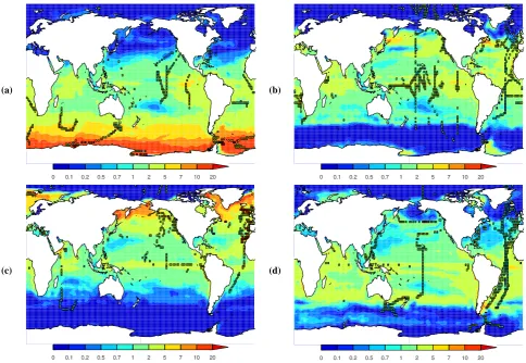
[image:13.595.75.530.56.209.2]total DMS-derived DMS-derived (%)
DJF
JJA
annual
[image:14.595.55.541.57.384.2]0 0.1 0.2 0.5 1 2 5 10 20 50 100 0 0.01 0.02 0.05 0.1 0.2 0.5 1 2 5 10 0 10 20 30 40 50 60 70 80 90 100
Fig. 8. Mean column burdens of SO2averaged for December, January and February (DJF) and June, July and August (JJA) and annual mean values resulting from all sources (total), resulting solely from DMS (DMS-derived) and percentage of SO2attributable to DMS (DMS-derived (%)), respectively. Units are mg(S)m−2and %, respectively.
Table 4. Annual mean column burdens of DMS, SO2, SO24−resulting from all sulfur sources (total) in (Tg(S)) and resulting only from DMS in (%).
annual mean December/January/ June/July/August
February
global NH SH global NH SH global NH SH
DMS (Tg(S)) 0.077 0.021 0.056 0.151 0.013 0.137 0.048 0.032 0.016
SO2total (Tg(S)) 0.604 0.414 0.190 0.642 0.440 0.202 0.592 0.400 0.192
% of SO2from DMS 24.7 15.7 44.2 28.8 15.0 58.9 21.0 15.8 31.25
SO24−total (Tg(S)) 0.733 0.493 0.240 0.674 0.363 0.311 0.813 0.617 0.195
% of SO24−from DMS 26.7 17.8 45.0 37.2 20.7 56.6 21.3 17.5 33.3
3.3.3 DMS contribution to SO2and SO24−column burdens
In order to quantify the importance of DMS-derived SO2and SO24−, we simulated the contribution of DMS-derived SO2 and SO24− to the total SO2 and SO24− concentration in the atmosphere. Additionally, this allows to utilize SO24− con-centration measurements in regions with a high DMS contri-bution for an evaluation of the DMS cycle.
SO2column burden
[image:14.595.112.486.482.580.2]total DMS-derived DMS-derived (%)
DJF
JJA
annual
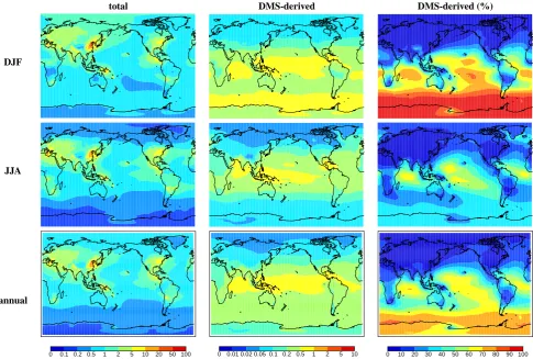
[image:15.595.55.543.58.384.2]0 0.1 0.2 0.5 1 2 5 10 20 50 100 0 0.01 0.02 0.05 0.1 0.2 0.5 1 2 5 10 0 10 20 30 40 50 60 70 80 90 100
Fig. 9. Mean column burdens of SO24−averaged for December, January and February (DJF) and June, July and August (JJA) and annual mean values resulting from all sources (total), resulting solely from DMS (DMS-derived) and percentage of SO24−attributable to DMS (DMS-derived (%)), respectively. Units are mg(S)m−2and %, respectively.
SO24−column burden in Fig. 9. The respective global mean column burdens are summarized in Table 4.
The global distribution of SO2column burdens resulting from all sources reflects the dominant anthropogenic sulfur sources in the Northern Hemisphere, most pronounced over the industrialized areas of Europe, North America and China. The SO2column burden resulting from DMS emission alone highlights the strong seasonal variation of DMS in the atmo-sphere. The highest column burdens persist in the Southern Hemisphere for December, January and February with val-ues up to 1 mg(S)m−2in high latitudes. The maximum in the Northern Hemisphere for June, July and August is less pronounced. In the equatorial regions, the SO2column bur-den attributable to DMS stays almost constant throughout the year. The simulated high DMS sea surface concentra-tion here causes a steady emission of DMS into the atmo-sphere and therefore a high load of SO2derived from DMS integrated over the atmospheric column. The relative contri-bution of DMS-derived SO2to the total SO2 shows clearly the overwhelming role of DMS in the Southern Hemisphere during the biological active season. In December, January and February the contribution is up to 90%.
The simulated global annual burden of SO2is 0.60 Tg(S), 25% of which can be attributed to DMS. Compared to the DMS contribution to the total sulfur emissions source, which is globally 30 %, the contribution of DMS to the SO2 col-umn burden is reduced. The contribution is greatest in the Southern Hemisphere (44%). The anthropogenic sources are dominant in the Northern Hemisphere. DMS accounts for 16% of the total SO2column burden on the annual mean in the Northern Hemisphere. Even in the summer months (June, July and August), when maximum DMS sea surface concen-trations are simulated in the Northern Hemisphere, the con-tribution of DMS to the total SO2column burden is greatest in the Southern Hemisphere (32% compared to 17% in the Northern Hemisphere).
SO24−column burden
-120 -60
0 60 120 180
[image:16.595.131.467.66.298.2]-90 -60 -30 0 30 60 90
Fig. 10. Location of the measurement sites included in the University of Miami network. Red points indicate stations with a simulated annual
mean DMS contribution to SO24−at the surface higher than 50%.
Pacific and the North Atlantic, occurs throughout the year. The SO24− column burden resulting from DMS emissions alone shows almost the same distribution as the SO2column burden resulting from DMS. A high burden persists in the Southern Hemisphere in the summer season. The export of SO24− into low emission regions causes a slight southward shift of the areas significantly influenced by DMS emissions. While for the SO2 burden a contribution of DMS of 60 to 70% for December, January and February is simulated in the equatorial regions of the Pacific and Atlantic, the contribu-tion for SO24−lies only between 40 to 50%.
The global annually averaged column burden of SO24− is 0.73 Tg(S) with a DMS contribution of 27% globally. The greatest contribution occurs in December, January and February with up to 37% globally and 57% in the South-ern Hemisphere. The DMS contribution to the SO24−burden lies within the same range as the DMS contribution to the SO2column burden. This is caused by the simulated strong chemical conversion rate of SO2to SO24−.
3.3.4 DMS-derived SO24−in the atmosphere
The global distribution of the fraction of the SO24−burden at-tributable to DMS shows the dominant role of DMS as SO24− precursor in the Southern Hemisphere, in particular at high latitudes (Fig. 9). A comparison of the simulated SO24− con-centrations with measurements in these remote regions there-fore gives an indication of the representation of the DMS cycle in the model simulation. Several measurement net-works include SO24− surface concentration measurements.
We choose the multi-annual measurements from the Univer-sity of Miami network (D. Savoie, personal communication), as this network includes mainly measurements from remote sites. These measurements have been conducted mainly on islands or at coastal stations. The number of measurement years varies with site. The measurement locations are dis-played in Fig. 10. Red points indicate stations with a simu-lated annual contribution of DMS to SO24−of more than 50% within the lowest model layer. These stations are mainly lo-cated in the Southern Hemisphere.
monthly annual
0.01 0.10 1.00 10.00 100.00
model SO4 [µg m-3]
0.01 0.10 1.00 10.00 100.00
measurement SO4 [
µ
g m
-3]
0.01 0.10 1.00 10.00 100.00
model SO4 [µg m-3]
0.01 0.10 1.00 10.00 100.00
measurement SO4 [
µ
g m
-3]
DJF JJA
0.01 0.10 1.00 10.00 100.00
model SO4 [µg m-3]
0.01 0.10 1.00 10.00 100.00
measurement SO4 [
µ
g m
-3]
0.01 0.10 1.00 10.00 100.00
model SO4 [µg m-3
] 0.01
0.10 1.00 10.00 100.00
measurement SO4 [
µ
g m
[image:17.595.122.473.61.382.2]-3]
Fig. 11. Scatter plot of measured and simulated surface aerosol mass concentration of SO24−. Measurements are from the University of Miami network. (a) Monthly mean, (b) annual mean, (c) mean for December, January and February, (d) mean for June, July and August. Red symbols indicate a contribution of DMS to SO24−higher than 50%. The solid line indicates the 1:1 ratio, the dashed lines the 1:2 and 2:1 ratios. Units areµg(S)m−3.
emission are high. DMS contributions higher than 50% ap-pear in 17 stations. For 12 stations with a contribution higher than 50%, the simulated values are a factor of 2 higher than the measured values. During the winter months (mean over June, July and August) DMS contributions higher than 50% exist for only 5 locations, 2 of which show higher simu-lated than measured values. In summary, for remote mea-surement stations the simulated SO24−surface concentrations are in agreement with the reported measurement values. Dis-crepancies from the observed values are highest for locations with a high DMS contribution, in particular in the summer season of the Southern Hemisphere. Here the model over-predicts the averaged observed concentrations by a factor of 2.3.
This overestimation may be caused by too high DMS emissions in these regions which are either due to too high DMS sea surface concentrations or too high sea-air exchange rates. The simulated DMS sea surface concentrations in summer in the Southern High Latitudes are very high com-pared to other regions of the ocean. Measurements reported from these regions confirm these high concentrations in the
Table 5. List of measurements sites from the University of Miami Network used in Fig. 11.
Location Longitude Latitude Model Measurements DMS contribution annual mean annual mean annual mean (µg m−3) (µg m−3) (%)
Chatham Island – New Zealand −176.5 −43.9 0.52 0.27 59
Cape Point – South Africa 18.5 −34.3 1.08 0.60 37
Cape Grim – Tasmania 144.7 −40.7 0.89 0.30 51
Iinverargill – New Zealand 168.4 −46.4 0.49 0.44 60
Marsh – King George Island −58.3 −62.2 0.38 0.27 52
Marion Island 37.8 −46.9 0.44 0.08 61
Mawson – Antarctica 62.5 −67.6 0.08 0.11 73
Palmer Station – Antarctica −64.1 −64.8 0.24 0.09 63
Reunion Island 55.8 −21.2 0.40 0.35 54
Wellingtin – New Zealand 174.9 −41.3 0.75 0.43 52
Yate – New Caledonia 167.0 −22.1 0.59 0.43 45
Funafuti – Tuvalu −179.2 −8.5 0.58 0.17 60
Nauru 166.9 −0.5 1.22 0.15 58
Norfolk Island 168.0 −29.1 0.51 0.27 55
Rarotonga – Cook Islands −159.8 −21.2 0.19 0.11 65
American Samoa −170.6 −14.2 0.25 0.34 64
Midway Island −177.4 28.2 0.46 0.52 33
Oahu Hawaii −157.7 21.3 0.73 0.51 33
Cheju – Korea 126.5 33.5 6.14 7.21 6
Hedo Okinawa – Japan 128.2 26.9 3.55 4.28 15
Fanning Island −159.3 3.9 1.17 0.64 48
Enewetak Atoll 162.3 11.3 0.37 0.08 55
Barbados −59.4 13.2 0.75 0.67 38
Izana Tenerife −16.5 29.3 2.40 0.96 22
Bermuda −64.9 32.3 1.03 2.09 22
Heimaey Iceland −20.3 63.4 0.47 0.69 26
Mace Head – Ireland −9.9 53.3 1.70 1.27 22
Miami −80.2 25.8 1.82 2.17 18
methyl sulfinic acid (MSIA) and methyl sulfonic acid (MSA) (Yin et al., 1990). A 1-D model study for marine boundary layer conditions (von Glasow and Crutzen, 2004) shows that the inclusion of halogen chemistry increases the DMS de-struction by about 25% in summer and 100% in winter time. The SO2yield from the oxidation of DMS is simulated lower when halogen chemistry is included. However, the lack of BrO measurements in the atmosphere makes a global assess-ment of the importance of the BrO oxidation difficult.
4 Summary and conclusions
The production of marine dimethylsulfide (DMS) and its fate in the atmosphere are simulated in a global coupled atmosphere-ocean circulation model. The processes for ma-rine DMS production and decay are included in the repre-sentation of plankton dynamics in the marine biogeochem-istry model HAMOCC5 embedded in a global ocean gen-eral circulation model (MPI-OM). The atmospheric model
ECHAM5 is extended by the microphysical aerosol model HAM.
The simulated DMS sea surface concentrations generally match the observed concentrations. The seasonal variation with its high DMS sea surface concentration in the high lat-itudes in the summer hemispheres is captured by the model. The global annual mean DMS sea surface concentration of 1.8 nmol l−1lies within the range of DMS sea surface clima-tologies (e.g. Belviso et al., 2004a).
with simulated values lower than the ones predicted from the Sim´o and Dachs (2002) algorithm.
The treatment of DMS in a coupled atmosphere-ocean model including a microphysical aerosol scheme and an atmospheric sulfur model allows to gain additional insight into the DMS representation in the model by a comparison with atmospheric DMS related measurements. The simu-lated DMS flux into the atmosphere is 28 Tg(S)yr−1which is in the range of current estimates (e.g. Kettle and Andreae, 2000). The resulting column integrated burden of DMS in the atmosphere is 0.08 Tg(S) and the lifetime is 1.0 days. DMS contributes 30% to the total sulfur source considered in the model (sulfur emissions from fossil- and bio- fuel use, wildfires and volcanoes and sulfur from DMS oxidation). The contribution of SO2derived from oxidation of DMS by OH and NO3to the total SO2column burden is 25%. SO2is oxidized by OH in the gas phase and by H2O2and O3in the aqueous phase to form SO24−. 27% of the produced SO24−can be attributed to DMS oxidation. The contribution is high-est in the biologically active season in remote regions of the Southern Ocean with values up to 90%.
The comparison of SO24− measurements and simulated SO24−concentrations at remote sites where the contribution of DMS to SO24−is generally high shows an overestimation of the SO24−surface concentrations by the model, most pro-nounced in the biologically active season. Possible explana-tions are an overestimation of the DMS sea surface concen-tration, a too high sea-air exchange rate or a missing reaction mechanism of DMS in the atmosphere. The simulated DMS sea surface concentrations are generally in agreement with the observations. A direct validation of the DMS flux is not possible because it cannot yet be measured directly. A miss-ing reaction of DMS in the atmosphere model is the reaction with BrO. It has been shown by several investigators that this reaction is important in remote regions (e.g. von Glasow and Crutzen, 2004; Boucher et al., 2003). However, the concen-tration of BrO in the atmosphere is not well known which makes a global assessment not feasible.
Future work will be to include the next step of the pro-posed DMS-climate feedback, i.e. the connection between aerosols and the cloud microphysics. The prognostic treat-ment of aerosol size distribution, composition and mixing state in the ECHAM5-HAM model provides the basis for such a microphysical coupling of the aerosol and the cloud scheme with an explicit simulation of cloud droplet and ice crystal number concentrations. For an assessment of the DMS-cloud link, it is important to consider sea salt and its role as CCN. Sea-salt emissions are high in regions with high DMS emissions and are also influenced by climate change.
The generally good agreement between model and mea-surements indicates that the DMS cycle in the model repre-sents the processes governing DMS sea surface tions, DMS emissions and resulting atmospheric concentra-tions reasonably well. However, the lack of measurements
of the consumption and production processes of DMS in the ocean hampers the full evaluation of the DMS formulation as a predictive tool for DMS. Nevertheless, the DMS for-mulation applied in a coupled ocean-atmosphere model is a step forwards in providing a model system to assess marine biosphere-climate feedbacks.
Acknowledgements. We wish to thank J. Prospero and D. Savoie (University of Miami) for providing the compilation of the multi-annual surface observations and J. Kettle for the maps of biogeochemical provinces. Many thanks to S. Legutke for the help with the OASIS coupler. We would also like to acknowledge the support of the German DEKLIM project funded by the German Ministry for Education and Research (BMBF) and the support of the International Max Planck Research School for Earth System Modelling. The simulations were done on the HLRE the High Performance Computing System for Earth System Research at the German Climate Computing Center (DKRZ).
Edited by: T. W. Lyons
References
Anderson, T. R., Spall, S. A., Yool, A., Cipollini, P., Challenor, P. G., and Fasham, M. J. R.: Global fields of sea surface Dimethylsulfide predicted from chlorophyll, nutrients and light, J. Mar. Systems, 30, 1–20, 2001.
Andreae, M. O. and Crutzen, P. J.: Atmospheric aerosols: Bio-geochemical sources and role in atmospheric chemistry, Science, 276, 1052–1058, 1997.
Andreae, M. O., Elbert, W., and Demora, S. J.: Biogenic sulfur emissions and aerosols over the tropical South-Atlantic. 3: At-mospheric Dimethylsulfide, aerosols and cloud condensation nu-clei, J. Geophys. Res., 100, 11 335–11 356, 1995.
Andreae, M. O., Elbert, W., Cai, Y., Andreae, T. W., and Gras, J.: Non-sea-salt sulfate, methanesulfonate, and nitrate aerosol concentrations and size distributions at Cape Grim, Tasmania, J. Geophys. Res., 104, 21 695–21 706, 1999.
Andres, R. J. and Kasgnoc, A. D.: A time-averaged inventory of subaerial volcanic sulfur emissions, J. Geophys. Res., 103, 25 251–25 261, 1998.
Archer, D. E. and Johnson, K.: A model of the iron cycle in the ocean, Global Biogeochem. Cycles, 14, 269–279, 2000. Archer, S. D., Smith, G. C., Nightingale, P. D., Widdicombe, C. E.,
Tarran, G. A., Rees, A. P., and Burkill, P. H.: Dynamics of par-ticulate Dimethylsulphoniopropionate during a lagrangian exper-iment in the northern North Sea, Deep-Sea Res., 49, 2979–2999, 2002.
Aumont, O., Belviso, S., and Monfray, P.: Dimethylsulfoniopro-pionate (DMSP) and Dimethylsulfide (DMS) sea surface distri-butions simulated from a global three-dimensional ocean carbon cycle model, J. Geophys. Res., 107, doi:10.1029/1999JC000111, 2002.