Trajectories Using Graph Databases
Rajesh Tamilmani
a,*, Emmanuel Stefanakis
ba Geodesy and Geomatics Engineering, University of New Brunswick, [email protected]
b Department of Geomatics Engineering, University of Calgary, [email protected]
* Corresponding author
Abstract: Geospatial databases are utilized in modelling the huge volume of spatial-temporal data generated by tracking moving objects equipped with positioning devices. This data can be used in performing trajectory analysis such as optimum path finding or identification of collision risk. At the same time, this massive data becomes difficult to handle using traditional databases as raw trajectories contain a lot of unnecessary data points. Thus, trajectory simplification techniques are applied to reduce the number of vertices representing a trajectory. However, elimination of intermediate points by simplification process leads to a loss of semantics associated with the trajectories. These semantics are dependent on the application domain. For example, a trajectory of a moving vessel can convey information about time, distances travelled, bearing, or velocity. This research proposes a graph data model that enriches the simplified geometry of trajectories with the semantics lost in the simplification process. Raw trajectories, initially modelled and stored in a PostgreSQL/PostGIS database, are simplified according to both their spatial and temporal characteristics using the Synchronized Euclidean Distance (SED), while the Semantically Enriched Line simpliFication (SELF) data structure is adopted to preserve the semantics of the vertices eliminated in the simplification process. Then, enriched simplified trajectories are transferred to a Neo4j database and modelled in terms of nodes and edges using graphs. Trajectories can then be further processed using Cypher query language and Neo4j spatial procedures. A visualization tool has been developed on top of Neo4j graph database to support the semantic retrieval and visualization of trajectories.
Keywords: trajectories, graph database, semantic, line simplification, modelling
1. Introduction
Positioning devices mounted on moving objects generate streams of geo-location data which describe the path travelled by each object during a period of time; this path is called trajectory. The advent of satellite technologies has enabled the wide usage of these devices on moving objects. Common application domains using trajectory data include city planning, transportation management systems, and other location-aware applications (Buchin et al. 2008). In the era of big data, graph databases address the major challenges in management and analysis of voluminous data. The concept of storing and representing data in terms of nodes, edges and properties makes graph databases different from relational databases and well suited for trajectory data management systems (Stefanakis 2017). Spatial analysis capabilities have already been added to graph database systems. For instance, Neo4j, one of the most prevalent graph database systems, provides a spatial plugin called Neo4j Spatial to facilitate spatial operations on geospatial data modelled using graphs (Neo4j Spatial Plugin 2017).
Over the last decade, researchers have focused on modelling and analysing raw trajectory data points using graph databases. Data reduction has always been
simplification process. The Semantically Enriched Line simpliFication (SELF) data structure has recently been proposed to retain the semantic attributes associated with individual locations of original trajectories (Stefanakis 2015).
The combination of the SELF data structure with the SED criterion has been implement-ed and tested in PostgreSQL/PostGIS using PL/pgSQL (Tamilmani and Stefanakis 2017). It has shown that semantics associated with the original trajectories are well retained in their simplified versions. The advent of graph databases (Neo4j 2017) has introduced an alternative and usually the more efficient way of modelling and analysing transportation data, including trajectory data, than traditional databases such as relational or object relational ones (Stefanakis 2017). This paper investigates the advantages of adopting a graph database to model and analyse the semantically enriched simplified trajectories generated by the combination of the SELF data structure with the SED criterion (Tamilmani and Stefanakis 2017). The enriched simplified trajectories are extracted from PostgreSQL/PostGIS databases and modelled into a Neo4j graph database. The nodes in the graph database are attributed with the semantic attributes (speed, heading, time, distances travelled, latitude and longitude) of the trajectories. The relationship(edges) between the nodes contain the intermediate accumulated simplified and original distances between consecutive vertices in the trajectory. These attributes are utilized in performing trajectory data analysis.
The contributions of this study are twofold. First, to propose a graph model for transfer-ring enriched simplified trajectories from PostgreSQL to Neo4j and further analysing them as graphs using Cypher query language (Neo4j 2017) and spatial procedures. The latter has been done by utilizing the Neo4j-spatial plugin that provides the geospatial analysis capabilities to Neo4j graph database (Neo4j Spatial Plugin 2017). Second, to support the semantic retrieval and visualization of modelled graph data in Neo4j. For this reason, a visualization tool has been developed on top of Neo4j for semantic interpolation at different levels of trajectory simplification.
2. Literature Review
2.1 Graph databases in trajectory data analysis Trajectories are formed by connecting series of raw mobility data points. These individual data points include temporal dimension apart from latitude and longitude. Over the years, tabular structured relational databases have been utilized in accommodating connected points forming trajectories. The relational data model and an extended Structured Query Language (SQL) was proposed for supporting the modelling and querying of real-world transportation networks. The comprehensive framework was built on top of Open Geospatial Consortium complaint (OGC-complaint) data models to support an algebraic-based network model. The proposed model has not addressed trajectories with millions of
points though (Hadi et al., 2014). In addition, relational databases lack in dealing with relationships because connectedness leads to increase in the number of joins between the tables, which in fact affects the performance of the database (Przemysław et al., 2016).
Graph databases help in leveraging the complex structure and dynamic relationships in connected trajectory data. The simple collection of nodes (vertices) and relationships (edges) facilitates the modelling of all varieties of data, from biological structures to the transportation data. Year by year the focus on utilizing graph databases in managing, processing and analysing spatial-temporal data has increased as the graph’s internal structure is in the form of a net-work (Gurfraind et al., 2016). Similar to SQL in relational databases, graph databases are also equipped with a multifaceted and robust query language for retrieving information. On the flip-side, visualizing all the nodes and edges would pose additional challenges as the graph layout is limited to display only certain number of nodes. Partl et al. (2016) presented a technique called “Pathfinder” for visualizing and analysing large graphs. The authors have followed a query-based approach for allowing the users to refine the data based on specific starting and ending nodes. However, the criteria for choosing these starting and ending nodes are not properly defined. With the graph databases, all the trajectory points are utilized in performing spatial analysis (Simplified trajectories are not utilized). Also, visualizing the million nodes and links makes it relatively hard for the user to understand the graphical layouts. It arises the issue of readability as the human visual capabilities are limited (Herman et al., 2000, Cui et al., 2007). This study is focused on analysing raw data points representing simplified trajectories us-ing the graph database. It is often required to reduce the tremendous amount of data points rep-resenting each trajectory. This process is also known as trajectory simplification. Also, the visualization tool has been developed on top of Neo4j graph database to support the semantic retrieval and visualization of trajectories. 2.2 Trajectory Simplification
The concept of reducing the number of points in a trajectory dataset is called trajectory reduction or simplification. The idea of trajectory reduction has evolved from cartographic generalization. Line simplification, the common cartographic generalization process, has been a key research area for cartographers over the years (Cromley 1991, Weibel 1997, Robinson et al. 2005, Wu et al., 2003).
The pre-processing step to add semantic information to the stops and moves is a time-consuming operation though the implemented model enables significant compression of trajectories. The semantic enrichment platform SeMiTri based on Hidden Markov Model (HMM) technique was developed with the provision of handling both fast and slow-moving objects (heterogenous trajectories). However, the multi-tiered approach has not considered scalability aspect of trajectories (Yan et al., 2011). Richter et al., (2012) proposed a system to enable users to determine the reference point and all possible movement change descriptions from that point. The authors extended network-constrained indexing to combine human movement with the individual positions on the trajectory. The pro-posed algorithm is only applicable to urban transportation networks.
The Douglas-Peucker (DP) algorithm has been criticized by many researchers. The problem of topological inconsistency between original and simplified geometry produced by DP algorithm was addressed by avoiding self-intersections on the simplified geometry (Wu et al., 2003). Even though most of the simplification algorithms consider only the perpendicular distance between data points and the proposed generalized version during simplification, these algorithms become inappropriate to be applied on trajectory datasets. This is mainly because they ignore the temporal characteristics of original trajectories. To remedy this, Meratnia and de By introduced the notion of Synchronous Euclidean Distance (SED) based simplification while reducing the number of vertices in the trajectory (2004).
The DP algorithm has been extended to resolve the problem of spatial relations violation while simplifying the trajectories. The extended algorithm retains the topological, direction and distance relations between the original and generalized trajectories (Stefanakis 2012, Tienaah et al., 2015).
2.3 Semantically Enriched Line Simplification (SELF)
SELF data structure has been introduced by Stefanakis (2015) to enrich the simplified line to convey semantics associated with the original version while achieving efficient generalization of trajectories by SED based simplification algorithm. The author has defined two variants in SELF structure based on how detailed the semantics to be attached with the simplified geometry. The basic variant of SELF attaches the original line length (e.g., kilometric travel distance) to the simplified line. In this variant, a line with end points 1 (start) and n (end), and total length (dn) will be represented by a
simplified line defined in Eqn. 1 (Stefanakis 2015). [x1, y1, xn, yn, dn] (SELF variant: basic) (1)
An advanced variant for function lines will also tag the accumulated length per vertex along the line. Hence, each vertex K of the original line will orthogonally be projected on the simplified line and the footprint point K’ will be assigned the accumulated length dk from point 1 (start) to vertex K along the original line. If dk’ is the
Euclidean distance of point K′ from end point 1, the simplified line will be represented in Eqn. 2 (Stefanakis 2015).
[x1, y1, xn, yn, dn, ARRAY {(dk’, dk); k=2, …, n-1}] (2)
In the attempt of enriching the content of the linear geometries while reducing the number of points, SELF data structure is implemented to preserve the length attributes associated with individual points on actual linear features (Tamilmani and Stefanakis 2017). The authors have implemented the advanced variant of SELF and tested the efficiency of the SELF structure with regard to geometric property preservation at various levels of simplification. The data structure has been implemented in PostgreSQL 9.4 using PL/pgSQL. The existing function in spatial ex-tension PostGIS 2.3 has been extended in implementing the SELF structure. For supporting the trajectory data enrichment, the advanced variant of the SELF structure has been extended to tag trajectory semantics: speed, heading, time and distance travelled. DP-SED algorithm works well for trajectory simplification as it retains the spatiotemporal characteristics of the trajectory. Each point on the original trajectory is projected on the generalized version based on SED. The footprint of each point will be assigned with speed, heading, time and distance travelled at that point (Eqn. 3).
[x1, y1, xn, yn, dn, ARRAY {(dk’, speed, heading,
time, dk); k=1, …, n}] (3)
3. Graph data model and analysis
Trajectories are formed by connecting series of raw mobility data points. Over the years graph databases have been used in analysing massive amounts of data generated by GPS devices mounted on mobility vehicles. For example, a trip duration of 60 minutes, with the location being recorded every 1 second, results in a total of 3,600 points. In a day trip, the dataset would contain 86,400 points. The number of nodes in the graph model is directly proportional to the number of points in the trajectory. Hence, it is necessary to reduce the volume of the dataset by applying trajectory simplification techniques.
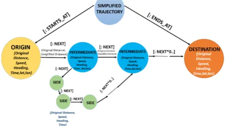
Figure 1: Proposed graph model for storing a simplified trajectory along with semantics using self-structure
has an origin and a destination. The starting and ending points of the original trajectory are converted into origin and destination nodes. The “INTERMEDIATE” nodes are attributed with original distance, speed, heading, time, latitude and longitude. In fact, these are the nodes which have been retained during the simplification process. The “SIDE” nodes have the following properties: original distance, speed, heading and time. These nodes represent the vertices which were eliminated during the simplification process. So, these nodes do not carry the latitude and longitude as properties. The main idea of keeping “SIDE” is to support trajectory reconstruction. The edges connecting two intermediate nodes are weighted with both the original and simplified distance between the corresponding points on the trajectory. The relationship between two nodes is labelled as “NEXT”. This study examines the modelling and analysis of enriched trajectories in a graph data-base. The approach involves three phases which are implemented in three system components.
Component 1: Transferring the simplified geometry of a trajectory and SELF structure from PostgreSQL/PostGIS to Neo4j graph database using JDBC
Component 2: Performing spatial and attribute analysis on the modelled data using Cypher query language and Neo4j spatial procedures.
Component 3: Visualizing the simplified trajectory in the web browser for semantic interpolation at different levels of trajectory simplification.
3.1 PostgreSQL/PostGIS to Neo4j bridging
The purpose of the first component in the overall system is to combine the simplified geometry of a trajectory with SELF structure and convert the simplified geometry into nodes and edges with the semantics stored as properties. The simplified geometry data from PostgreSQL/PostGIS is mapped into Neo4j graph database using Java Database Connectivity (JDBC). This component is implemented in the following three steps.
3.1.1 Simplifying the trajectory based on Synchronous Euclidean Distance
SELF structure for dynamic lines stores the semantics associated with individual points on the original trajectory along the simplified version. As shown in the Fig.2, each point on the original trajectory is projected based on the SED to the simplified version. The sample trajectory shown in Fig.2 has 10 points in the original version, while the simplified version retains 7 points.
Figure 2: Example original and simplified trajectories
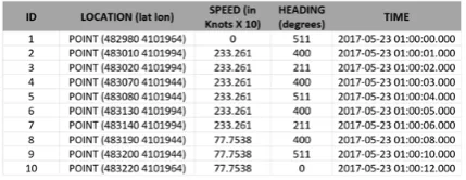
For each vertex on the original trajectory, the corresponding SED point is tagged with the semantics given in Table. 1 (Tamilmani and Stefanakis 2017).
Table 1. Attribute table for the trajectory points shown in Figure 2 The entire SELF structure is represented as follows
3.1.2 Generating nodes and edges from simplified geometry
Once the trajectory is simplified each point on the simplified geometry is compared with the points on the original trajectory to decide the node type. The points which were eliminated dur-ing the simplification are labelled as “SIDE” nodes and the retained points are labelled as “INTERMEDIATE” nodes, while the starting and ending points of the trajectory are labelled as “ORIGIN” and “DESTINATION” nodes. The “SIDE” nodes do not contain latitude and longitude, whereas all other nodes contain the spatial coordinates as these nodes represent the points which have been retained by the simplification algorithm (Fig. 3). In our example, the points 2, 7 and 9 were eliminated during the simplification process (Fig. 2). So, these nodes are labelled as “SIDE”. The remaining nodes representing points 3, 4, 5, 6 and 8 are labelled as “INTERMEDIATE”. The first and last nodes are labelled as “ORIGIN” and “DESTINATION”.
Figure 3: Labelling the nodes based on the corresponding retained or eliminated points
3.1.3 Associating the nodes and edges with semantics from SELF structure
Once the nodes have been labelled, the SELF structure has to be parsed along with the simplified geometry to add the associated semantics as properties to the nodes. Algorithm 1 associates the nodes and edges with semantics from the SELF structure. The developed algorithm takes the simplified geometry and the SELF structure as input to add the properties to the nodes. The accumulated length at every point on the simplified trajectory is calculated and stored in an array. Each simplified distance in the SELF structure is searched through the accumulated length array. If a match is found,
[ SPOINT (482980 4101964), EPOINT (483220 4101964), 322.843,
{(0.000,0,511,0.00, 2017-05-23 01:00:00.000), (30.594,233.261,400,42.426, 2017-05-23 01:00:01.000), (61.188,233.261,211,52.426, 2017-05-23 01:00:02.000), (91.782,233.261,400,123.137, 2017-05-23 01:00:03.000),
(122.376,233.261,511,133.137, 2017-05-23 01:00:04.000), (152.971,233.261,400,203.848, 2017-05-23
then that node is labelled as “INTERMEDIATE” and attributed with the corresponding latitude, longitude, speed, heading, time and distance travelled as extracted from SELF structure. If the accumulated length does not match with simplified distance in the SELF structure, then that node is labelled as “SIDE” and attributed with the corresponding speed, heading, time and distance travelled from the SELF structure.
Two separate CSV (Comma-Separated Values) files have been generated for uploading the trajectory data into Neo4j. One of them (all_nodes.csv) is for loading the nodes, and the other (all_edges.csv) is for connecting these nodes with edges. Any two consecutive intermediate nodes are connected by an edge which is weighted with the original and simplified distance between those nodes.
The generated nodes are then uploaded to Neo4j graph along with the properties using the Cypher query. Nodes are connected by edges after uploading edges CSV file to Neo4j graph using the Cypher query.
The generated graph represents the enriched simplified trajectories using nodes and edges. Fig. 4 shows a sample trajectory graph in Neo4j.
INTERMEDIATE nodes are labelled with the order of the corresponding point in the simplified geometry. The SIDE nodes are identified by an ID which follows the naming convention:
(INTERMEDIATE_NODE_ID)_(NEXT_INTERMEDIATE_NODE_ID)_(COUNT). For
instance, the SIDE node with ID “5_6_1” denotes that is the first node lost during simplification between the intermediate nodes 5 and 6.
Figure 4. Generated graph data showing the nodes and edges
3.2 Spatial analysis using Cypher
The uploaded trajectory data into Neo4j can be analysed using Cypher query language and Neo4j spatial procedures. Here is a list of example queries that Neo4j can support:
1. Finding the shortest and longest trajectory based on: •Number of nodes
•The original distance between origin and destination •The time difference between origin and destination 2. Identifying the overall collision region between trajectories:
•Identifying the collision region at a time interval
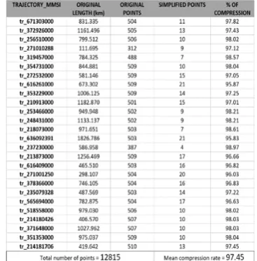
The SED based simplification was carried out over a dataset of vessel trajectories for August 2013 in the Aegean Sea as collected by the MarineTraffic Automatic Identification System (AIS) (MarineTraffic 2017) and the number of points retained after simplifying (with a threshold = 10km) is shown in Table 2. Simplification threshold has been chosen as 10 km based on the length of individual trajectories. The average length of all the trajectories is around 1000.0 km, so to achieve a higher simplification the small threshold value (10 km) has been chosen. Individual trajectories are identified by “MMSI” which is unique for the moving vessel. From Table 2, it is evident that the simplification step has reduced the number of points in the original trajectories.
Each simplified trajectory was associated with the SELF structure, modelled into the graph database, and used for further analysis to prove that not all the raw points in a trajectory are necessary to perform trajectory analysis. Trajectories with a variable number of mobility data points have been chosen so that the representative set of features with a wide range of spatial-temporal characteristics is analysed.
Table 2. Number of points in the original and simplified trajectory
3.2.1 Finding shortest and longest trajectory
The path in the graph is defined as the sequence of nodes which are connected by weighted or non-weighted edges. In this model, edges are weighted with both the original and simplified distance between consecutive simplified points.
3.2.2 Compression ratio based on the number of nodes connected between origin and destination
The sequence of nodes which are connected between the origin and destination is count-ed to determine the length of the trajectory. This connectivity measurement is carried out on all the individual trajectories in the modelled data.
Then the trajectory with the highest number of nodes between origin and destination is chosen as the longest and vice versa.
trajectory with the highest number of nodes between origin and destination is chosen as the longest and vice versa.
FOREACH (simplified_trajectory IN graph)
MATCH (origin: simplified_trajectory)-[c]->(destination: simplified_trajectory)
WHERE origin.id = destination.id RETURN origin.name, COUNT(c) ORDER BY COUNT(c) ASC/DESC;
By finding the ratio between the total number of nodes (including “SIDE” nodes) be-tween origin and destination against the count of “INTERMEDIATE” nodes, this will be an interesting parameter to know how much the trajectory has been simplified.
FOREACH (simplified_trajectory IN graph)
MATCH (origin: simplified_trajectory)- [c]->(destination: simplified_trajectory) , (orig: simplified_trajectory{nodeType: ‘SIDE’})- [d]->(dest: simplified_trajectory{nodeType: ‘SIDE’}) WHERE origin.id = destination.id AND orig.id = dest.id RETURN origin.name, COUNT(c)/COUNT(d)
ORDER BY COUNT(c) ASC/DESC;
3.2.1.2 Shortest/longest trajectory based on original distance between origin and destination
The accumulated distance between the sequence of nodes which are connected between the origin and destination determines the length of the trajectory. This geometry measurement is done on all the individual trajectories in the modelled data. Then, the trajectory with the longest distance is chosen as the longest and vice versa. The below query sums up the original distance weight in all the edges for each trajectory to determine the original length of the trajectory. Then, it finds three shortest/longest trajectories by ordering the calculated distance in ascending/descending order. Also, the length of the simplified trajectory can be easily calculated by reading origDist attribute in the edge connecting to the DESTINATION node. The results are shown in Table 3 and 4 matches with the shortest/largest trajectories identified using QGIS (Fig. 5 & 6).
FOREACH (simplified_trajectory IN graph)
MATCH(origin:simplified_trajectory)-[c:NEXT]->(destination: simplified_trajectory)
WHERE origin.id=destination.id AND origin.type = ‘intermediate’
RETURN origin.name, sum(toFloat(c.origDistWeight)) ORDER BY sum(toFloat(c.origDistWeight)) ASC/DESC LIMIT 3;
Table 3. Results of shortest trajectories based on the length
Table 4. Results of longest trajectories based on the length
Figure 5: Shortest trajectories identified in QGIS based on length matches the results of cypher query in table 3.
Figure 6: Longest trajectories identified in QGIS based on length matches the results of cypher query in table 4.
3.2.1.3 Shortest/longest trajectory based on original distance between origin and destination
The time difference between the sequence of nodes which are connected between the origin and destination determines the total time duration of the trip. This temporal measurement is done on all the individual trajectories in the modelled data. Then, the trajectory with the higher time difference is chosen as the longest and vice versa.
The below query calculates the time difference between origin and destination for each trajectory to determine the total travel time of a trajectory. The time difference is then sorted in ascending/descending order to find the three shortest/longest trajectories.
FOREACH (simplified_trajectory IN graph) MATCH (origin: simplified_trajectory)-[c:NEXT]->(destination: simplified_trajectory)
WHERE origin.id = destination.id
RETURN origin.name, (destination.time – origin.time) ORDER BY (destination.time – origin.time) ASC/DESC LIMIT 3;
3.2.3 Identifying the collision region
SPATIAL.CLOSEST finds all geometry nodes in the graph within the distance to the given coordinate (Neo4j Spatial Plugin 2017). The following Cypher query finds the corresponding number of nodes within particular distance for each node and identifies the point with the maximum number of neighbours.
MATCH (tr:TrajectoryNodes) WITH tr
CALL SPATIAL.CLOSEST(‘spatial_graph’',{latitude: tr.latitude, longitude: tr.longitude},10000)
YIELD node WHERE node.trid <> tr.trid
RETURN tr, COUNT(node) ORDER BY COUNT(node) DESC LIMIT BY 1;
The results from Cypher query have been compared against the buffer operator in QGIS. The number of points falling within the buffer region (34) is same as the number of neighbors identified by Neo4j.
By enforcing the temporal constraint, the above query can be extended to find the collision region for a given time period of a day. The following sample will identify the collision point between 4 pm and 8 pm.
MATCH (tr: TrajectoryNodes) WITH tr
CALL SPATIAL.CLOSEST(‘spatial_graph’',{latitude: tr.latitude, longitude: tr.longitude},10000)
YIELD node WHERE node.trid <> tr.trid and node.day = tr.day and hour>16 and hour<20
RETURN tr, COUNT(node) ORDER BY COUNT(node) DESC LIMIT BY 1;
3.3 Visualization tool for semantic interpolation A web-based graph data visualization system has been developed for visualizing the simplified trajectory and retrieving semantics using the proposed model. The dynamic system allows the user to choose the trajectory on which the semantic retrieval will be performed. The graph visualization capabilities have been added using the JavaScript framework “alchemy.js”. Alchemy is a graph visualization tool for developing web applications. It is easily customizable and includes the capabilities like clustering, filtering and embedding graphs (Alchemy 2017).
An HTML powered web application allows the user to select single trajectory from a collection of trajectories. The browser then sends the corresponding HTTPS request to a RESTful Webservice through an Angular-based web page (Angular 2017). The request is then parsed by Apache server before it hits Neo4j database for retrieving the corresponding graph as an object. Java-Neo4j-API lets the Java program communicate with Neo4j database. The response is a JSON (JavaScript Object Notation) object that is then parsed by Alchemy to display the graph data on the browser. The following snapshots summarize the functionality of the developed system. The user can choose a single trajectory from the dropdown list of trajectories.
The visualization architecture is shown in Fig.7. After a trajectory is selected by the user, the corresponding graph data can be visualized on the browser screen. Once the database responds with proper data, the object received by Apache server is sent to alchemy.js as a JSON object.
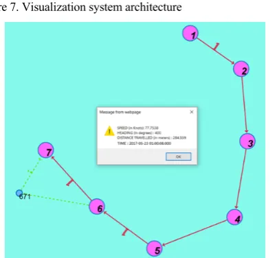
Alchemy framework enables the browser to parse the JSON object. Numeric value on the edges denotes the number of points eliminated during the simplification between those edge nodes.
In this example between node 6 and 7, there was one point which is lost during the simplification of the trajectory. If the user clicks on that number, the corresponding node (“SIDE”) which has been lost will also be displayed.
The nodes in pink circles connected by red coloured edges represent “INTERMEDIATE” points, while the nodes in green connected by dotted green edges represent “SIDE” points. The user can click on any node to retrieve its corresponding semantics, such as speed, heading, distance travelled and time of crossing (Fig.8).
Figure 7. Visualization system architecture
Figure 8. Alert box with the semantics for the clicked point
4. Conclusions
Visualization of massive trajectory datasets becomes difficult to handle as the large amount of raw data points makes the processing complex. The proposed graph model for combining the simplified geometry of trajectories and SELF data structure has facilitated the trajectory data analysis using Cypher query language and Neo4j Spatial procedures. The visualization tool developed on top of Neo4j provides useful functionality that can be extended to support different application domains.
More emphasis on evaluating the time complexity of the implemented algorithms with various compression levels being applied to the SELF structure will make the running time optimal. Both the graph model and developed visualization framework can be applied to various application domains such as bus transit and metro systems. The visualization tool can be extended to display the trajectories on geographic base maps.
5. References
Alvares, L.O., et al., (2007). A model for enriching trajectories with semantic geographical information. In: The Proceedings of the 15th annual ACM international symposium on advances in geographic information systems, 7–9 November, Seattle, WA. Article No. 22.
Buchin, K., Buchin, M., and Gudmundsson, J., (2008). Detecting single file movement. In GIS '08: Proceedings of the 16thACM SIGSPATIAL international conference on Advances in geographic information systems, pages 1-10, New York, NY, USA.
Cromley, R.G., (1991). Hierarchical methods of line simplification. Cartography and Geo-graphic Information Science, 18 (2), 125–131. doi:10.1559/152304091783805563 Cui, W and Qu, H, A survey on graph visualization, PhD
Qualifying Exam (PQE) Report, (2007). Computer Science Department, Hong Kong University of Science and Technology, Kowloon, Hong Kong, 2007.
Gurfraind, A., and Genkin, M., (2016). A graph database framework for covert network analysis: An application to the Islamic State network in Europe. World Development, Pages1-11doi: 10.1016/j.socnet.2016.10.004
Hadi, H., and Farshad, H., (2014). A Spatial Data Model For Moving Object Databases, International Journal of Database Management Systems (IJDMS ) Vol.6, No.1, February 2014,doi:: 10.5121/ijdms.2013.6101 1
Herman. I, Melancon. G, and Marshall M.S, Graph visualization and navigation in information visualization: A survey, (2000)," Visualization and Computer Graphics, IEEE Transactions on, vol. 6, no. 1, pp. 24-43, 2000.
Keates, J.S., (1989). Cartographic design and production. 2nd ed. Essex: Longman.
MarineTraffic, (2017). Live-ships map: AIS [online]. Available from: http://www.marinetraffic.com/ais/ [Last visited, June 27, 2017]
Meratnia, N., and de By, R.A., (2004). Spatiotemporal compression techniques for moving point objects. In: Proceedings of the international conference on extending database technology (EDBT). Berlin: Springer, 765–782. LNCS 2992.
Neo4j Spatial Plugin, http://neo4j-contrib.github.io/spatial/0.24-neo4j-3.1/index.html, Ac-cessed on: 17th August 2017
Neo4j Graph Database, https://neo4j.com/, Accessed on: 1st August 2017
Parent, C. et al., (2013). Semantic Trajectories Modeling and Analysis. ACM Computing Surveys, Vol. 45, No.4, Article 42. doi: http://dx.doi.org/10.1145/2501654.2501656
Partl, C., Gratzl, S., Streit, M., Wassermann, A.M., Pfister, H., Schmalstieg, D., and Lex, A., (2016). Pathfinder: Visual Analysis of Paths in Graphs Eurographics Conference on Visualization (EuroVis) 2016 Volume 35 (2016), Number 3 Przemysław, I., et al. (2016). Visualization of Relational
Database Structure by Graph Database CMST 22(4) 217-224 doi:10.12921/cmst.2016.0000014
QiuLei Guo and Hassan A. Karimi, (2016). A Topology-Inferred Graph-Based Heuristic Algorithm for Map Simplification. In: Transactions in GIS, doi:10.1111/tgis.12188
Richter, K.F., Schmid, F., and Laube, P., (2012). Semantic trajectory compression: repre-senting urban movement in a nutshell. Journal of Spatial Information Science, (4), 3–30. Robinson, A.H., Joel L. Morrison, Phillip C. Muehrcke, A. Jon
Kimerling, Stephen C. Guptill. (1995). Elements of Cartography, 6th Edition ISBN: 978-0-471-55579-7
Shahriari, N., and V. Tao. (2002). Minimizing Positional Errors in Line Simplification Using Adaptive Tolerance Values. In: Symposium on Geospatial Theory, Processing and Application, 4(3), 213-223.
Spaccapietra, S., et al., (2008). A conceptual view on
trajectories. Data & Knowledge Engineering, 65 (1), 126–146. Stefanakis, E., (2017). Graph Databases – Recent development in Neo4j may help accommodate the Geospatial Community. GoGeomatics. Magazine of GoGeomatics Canada. January 2017.
Stefanakis, E., (2012). Trajectory generalization under space constraints. In: The proceedings of the 7th international conference on geographic information science (GIScience 2012), 18–21 September, Columbus, OH.
Stefanakis, E., (2015). SELF: Semantically enriched Line simpliFication. In: International Journal of Geographical Information Science, Vol. 29, Iss. 10, 2015, Pages 1826-1844 doi: 10.1080/13658816.2015.1053092
Tamilmani, R., Stefanakis, E., (2017). Enriched geometric simplification of linear features. Geomatica Vol. 71, No.1, 2017, pp. 3 to 19. doi: dx.doi.org/10.5623/cig2017-101 Tienaah, T., Stefanakis, E., and Coleman, D., (2015).S
Contextual Douglas-Peucker simplification. Geomatica Journal, 69 (3), 327-338, https://doi.org/10.5623/cig2015-306 Weibel, R., (1996). A typology of constraints to line
simplification. In: Proceedings of 7th international symposium on spatial data handling, 12–16 August, Delft. IGU, 533–546. Weibel, R., (1997). Generalization of spatial data: principles
and selected algorithms. In: M. Kreveld, et al., eds. Algorithmic foundations of geographic information systems. Berlin: Springer, 99–152.
Wu, et alShil – Ting and Mercedes Rocio Gonzales Marquez (2003). Proceedings of the XVI Brazilian Symposium on Computer Graphics and Image Processing (SIBGRAPI’03) 1530-1834/03 doi :10.1109/SIBGRA.2003.1240992