Design and analysis of computer experiments using polynomial regression and Latin hypercube sampling in optimal design of PID controller

(1)

1. Introduction

Nowadays, simulation-optimization methods based on DACE have been commonly interested in displaying the performance of the complex system [1]. The essential benefit of DACE method is its ability to cover complex processes in order to avoid intensive computational complexity which might squander time and resource for estimating model's parameters. There are different ways for designing of systems optimally via a mathematical model, simulation model, or meta-model. Two difficulties which arise from existing methods are computational complexity to find an optimal design and

_{Corresponding author}

E-mail address: [email protected]

DOI: 10.22105/jarie.2018.141898.1051

Design and Analysis of Computer Experiments Using Polynomial

Regression and Latin Hypercube Sampling in Optimal Design of

PID Controller

Amir Parnianifard, Siti Azfanizam Ahmad, Mohd Khairol Anuar Ariffin, Mohd Idris Shah Ismail

Department of Mechanical and Manufacturing Engineering, Faculty of Engineering, Putra MalaysiaUniversity, 43400 UPM Serdang, Selangor, Malaysia.

A B S T R A C T P A P E R I N F O

Computational complexity and time-consuming iteration of simulation for tuning of Proportional-Integral-Derivative (PID) controller is a common drawback in many types of existing methods. This paper aims to propose a new method for achieving an optimal design for PID gains parameters with the least number of simulation runs. To achieve this purpose, we combine polynomial regression and Latin Hypercube Sampling (LHS) in order to Design and Analyze of Computer Experiments (DACE). In this method, the LHS is performed three times to design the associated sample points for different usage that includes training sample points to fit polynomial regression as a common surrogate model; validating sample points to scale standardized residuals; grid search sample points for investigating optimal point over whole design space. To show the flexibility and applicability of the proposed method, we serve a numerical case in the tuning of PID controller for linear speed control of Direct Current (DC) motor. Four different polynomial regression fit input/output (I/O) data over separately four model’s performances that includes Square-Error (ISE), Absolute-Error (IAE), Integral-Time-Square-Error (ITSE), and Integral-Time-Absolute-Error (ITAE). Comparison of the result with two existing approaches such as traditional Zeigler-Nichols method and Taguchi-Gray Relational Analysis (Taguchi-GRA) confirms the reliability and superiority of the proposed method.

Chronicle:

Received: 23 April 2018 Accepted:11 August 2018

Keywords:

Polynomial Regression. PID Controller. DC Motor.

Simulation Optimization. Computer Experiments. Latin Hypercube Sampling.

Journal of Applied Research on Industrial

Engineering

(2)

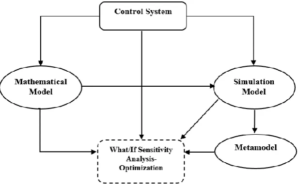
consuming due to a large number of model’s iterations [2]. Notably, choosing the best way depends on the amount of complexity in the system; see Fig. 1.

Fig. 1. Different ways for optimizing a control system based on mathematical, simulation, or metamodel.

However, different methods have been proposed in literature for designing of PID controllers optimally (e.g. evolutionary methods and heuristics algorithms); see [3]. Yet, investigating less computationally expensive methods less computationally for tuning of PID controller has been a main challenging issue in the world of control systems [4]. If the complex system not costly worth, it to be derived physically for tuning of PID controller; computer experiments through simulation model can be performed to extract approximation model instead of the real model. In such a case, metamodels (also called surrogate models) can appropriately be used to reduce the computational complexity in designing of PID controller [5]. There are several metamodels in literature applied in engineering optimization that are polynomial regression, Kriging, and Radial Basis Function (RBF) commonly [6, 7]. Undoubtedly, the most common and easy use of metamodel in simulation-optimization is polynomial regression (also called response rurface methodology) that can successfully be applied in various types engineering problems [8]. However, the tuning of PID controller applying polynomial regression has been attended in some studies; see [9-12].

Computer experiments are conducted as main supplementary of meta

_-

model based robust simulation optimization. The strength of metamodel like polynomial regression strongly depends on appropriate designing of relevant sample points which used to fit model [13]. Among different approaches for designing computer experiments, LHS has become most well-known than others [14]. LHS can cover whole design space that leads to space filling experimental design.

(3)

generally for tuning of PID controllers in most types of control systems. This paper focuses on the optimal designing of PID controller for linear speed control of DC motor. DC motors have been widely employed as actuating sources in industrial application. DC motor systems with their electromechanical components are widely employed in various industrial applications due to their advantages such as easy speed control, position control, and wide adjustability interval. The new method is compared to some other types of approaches in tuning of PID controller such as metaheuristic methods [16], genetic algorithms [17], particle swarm optimization [18], fuzzy technique [19], and Taguchi method [20]. The application of metamodels (e.g. polynomial regression) has been less attended in case of complex simulations particularly using DACE.

The remainder of this paper is organized as follows: A basis of Metamodel-Based Simulation Optimization (MBSO) including polynomial regression and LHS is briefly explained in Section 2. Section 3 contains a description of PID controller for speed control of DC motor. In Section 4, the proposed MBSO algorithm to perform optimization model sketched out parallel to numerical case study in optimal design of PID controller for speed control of DC motor. Note that, the proposed polynomial regression-based optimization model consists of designing the computer experiments with LHS method, fitting polynomial regression metamodel, validating metamodel, and applying the grid search over whole design space. Finally, Section 5 is the conclusion section of this paper.

2. Metamodel Based Simulation Optimization (MBSO)

The system behavior is evaluated by running a simulation model for a fixed period of time which called computer experiments (also called simulation experiments). Metamodel can be fitted over I/O data which resulted in simulation experiments. Here, we use polynomial regression as the most common metamodel to approximate simulation and fit I/O data. The most advantages of polynomial regression are compared with other metamodels like Kriging and RBF [8]:

 The application of polynomial regression has been confirmed by large number of case studies in different engineering problems.

 Polynomial is supported by appropriate commercial software.

 Gives more information about model’s parameters such as main effect of input variables and interaction between variables.

 Handlling sensitivity analysis of model’s parameters is easy.  Supports stochastic simulation in uncertain and noisy environment.

However, in order to guarantee the validity of metamodel, the design of training sample points needs to be done over whole design space appropriately. The traditional design of experiment method for polynomial regression (e.g. Central Composite Design (CCD), Box-Behnken, and so on) [21] is not suitable for deterministic simulation, because with the same input combination by any number of re-running the model, the fixed output is gained. Moreover, here LHS as the modern method for designing of simulation experiments is used instead of the traditional methods.

2.1. Latin Hypercube Sampling (LHS)

(4)

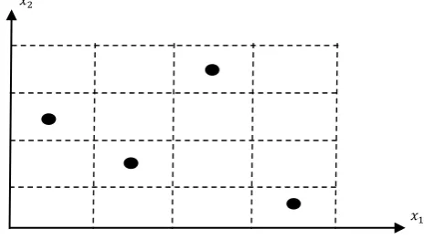
(with equal probability). For the particular instance, the LHS design for 𝑚 = 4, 𝑛 = 2 is shown in Fig. 2.

Fig. 2. An example for LHS design with two input factors and four intervals.

The LHS strategy proceeds as follows:

 In LHS, each input range divided into 𝑚 subranges (integer) with equal probability magnitudes and numbered from 1 to 𝑚. In general, the number of 𝑚 is larger than total sample points in CCD.

 In the second step, LHS permutes all 𝑚 intervals by random value between lower and upper bounds relevant to each interval, since each integers 1,2, … , 𝑚 appears exactly once in each row and each column of the design space. Note that, within each cell of design, the exact input value can be sampled by any distribution, e.g. uniform, Gaussian, etc.

In this context for our proposed method, the LHS is performed three times to produce the needed sample points [15] by different usage that includes training sample points; validating sample points; search sample points. Training sample points are run by the original simulation model and obtained data are used for fitting metamodel. Validating sample points are run with both original simulation model and metamodel, and the extracted data employed for metamodel validating. Search sample points are run just by metamodel and the extracted data are applied in the global search to find optimal point.

2.2. Polynomial Regression

Polynomial regression is a collection of statistical and mathematical techniques useful for developing, improving, and optimizing the process. The functional applicability of polynomial regression in literature can approximate the relationship between design (dependent) variables and single or multi-response (independent variables), investigate and determine the best operating condition for the process by finding the best levels of design region which can satisfy operating limits, and implement robustness in the response(s) of the process by designing the process robust against uncertainty. Commonly, the main motivation of polynomial approximation for true response function is based on Taylor series expansion around a set of design points [21]. The general overview of the first-order response surface model is shown as:

where 𝑘 is the number of design variables. Most times, the curvature of response surface is stronger than the first model that can approximate it even with the interaction terms. So, a second-order (quadratic) model can be employed:

𝑦 = 𝑓(𝑋) = 𝛽̂0+ ∑ 𝛽̂𝑖 𝑘

𝑖=1

𝑥𝑖+ 𝜀 (1)

𝑥2

(5)

𝑦 = 𝑓(𝑋) = 𝛽̂0+ ∑ 𝛽̂𝑖 𝑘

𝑖=1

𝑥𝑖+ ∑ 𝛽̂𝑖𝑖 𝑘

𝑖=1

𝑥𝑖2+ ∑ ∑ 𝛽̂𝑖𝑖′

𝑘

𝑖<𝑖′₌₂

𝑘

𝑖=1

𝑥𝑖𝑥𝑖′+ 𝜀 (2)

where 𝛽̂0, 𝛽̂𝑖, 𝛽̂𝑖𝑖 and 𝛽̂𝑖𝑖′ are unknown regression coefficients and the term 𝜀 is the usual random error (noise) component; see [21].

3. PID Controller for Linear Speed Control of DC Motor

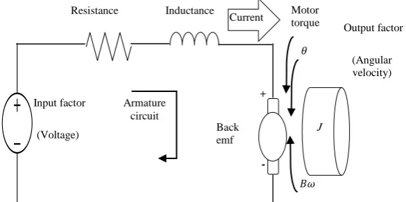
A DC motor is constructed with two sub-systems. The first sub-system is electrical part and consists of armature inductance, armature resistance, and the magnetic flux of the stator. The mechanical motor is the second sub-system that consists of the inertia of the motor and a load. Changing in the motor speed is due to electromagnetic moment made by the amplifier current, load, and the friction of the motor. Fig. 3 shows the simplified electrical circuit of DC motor and the mechanical model of a rotor.

Fig. 3. An electrical and mechanical components of DC motor.

The dynamic behavior of DC motor based on the mathematical model is expressed by:

𝐽𝑑𝜔(𝑡)

𝑑𝑡 + 𝐵𝜔(𝑡) = 𝑇𝑚(𝑡) (3)

𝐿𝑑𝑖𝑎(𝑡)

𝑑𝑡 + 𝑅𝑖𝑎(𝑡) = 𝑣𝑎(𝑡) − 𝑣𝑏(𝑡) (4)

𝑣𝑏 = 𝐾𝑒𝜔(𝑡) (5)

𝑇𝑚(𝑡) = 𝐾𝑡𝑖𝑎(𝑡). (6)

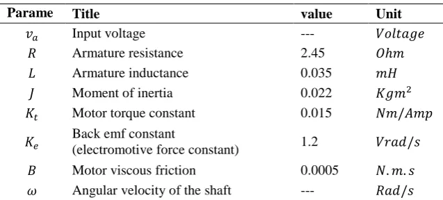
We modeled DC motor in MATLAB®_{Simulink toolbox by load parameters which are depicted in Table}

1.

- Armature

circuit

Inductance

+

Back emf Resistance

Input factor

(Voltage) J

Current Motor _torque

𝜃

𝐵𝜔

Output factor

(6)

Table 1. Load parameters in DC motor system.

Here, we use the same example with [20] to show the analytical comparison between our proposed method, classical tuning by Ziegler-Nichols method, and the method proposed by [20] which combined Taguchi approach and gray relational analysis (Taguchi-GRA). The PID controller employs three terms of proportional, integral and derivative to reduce an error signal (𝑒) to be more close to zero. The output of a PID controller, equal to the control input to the plant, in the time-domain is as follows:

𝑢(𝑡) = 𝐾𝑝𝑒(𝑡) + 𝐾𝑖∫ 𝑒(𝑡)𝑑𝑡 + 𝐾𝑑

𝑑𝑒 𝑑𝑡

𝑡

0

(7)

The appropriate function of PID strongly depends on allocated magnitude to each gain of 𝐾𝑝, 𝐾𝑖, and

𝐾𝑑. In order to evaluate the performance of PID controller, four common creations are used. Note that all creations are associated with all time-response parameters included rise time, steady state error, settling time, and overshoot [23]. The mathematically features of performance creations in time domain are defined as below:

𝑀𝑖𝑛 𝐼𝑆𝐸 = ∫ 𝑒(𝑡)2_𝑑𝑡 ∞

0

(8)

𝑀𝑖𝑛 𝐼𝐴𝐸 = ∫ |𝑒(𝑡)|𝑑𝑡

∞

0

(9)

𝑀𝑖𝑛 𝐼𝑇𝑆𝐸 = ∫ 𝑡. 𝑒(𝑡)2_𝑑𝑡 ∞

0

(10)

𝑀𝑖𝑛 𝐼𝑇𝐴𝐸 = ∫ 𝑡. |𝑒(𝑡)|𝑑𝑡

∞

0

(11)

In above equations, 𝑒(𝑡) = (𝑦(𝑡) − 𝑆𝑝), where 𝑦(𝑡) is response (output) in time 𝑡 and 𝑆𝑝 is desired set point for response of model (i.e. here the rotational speed is defined as an output in the DC motor system).

4. MBSO Algorithm

Inspired by [1, 24], the MBSO algorithm is sketched out in some steps as follows. Here, we extend this approach for the tuning of PID controller for linear speed control of DC motor (i.e. the magnitudes of load’s parameters are stated in Table 1).

Parame ter

Title value Unit

𝑣𝑎 Input voltage --- 𝑉𝑜𝑙𝑡𝑎𝑔𝑒 𝑅 Armature resistance 2.45 𝑂ℎ𝑚 𝐿 Armature inductance 0.035 𝑚𝐻

𝐽 Moment of inertia 0.022 𝐾𝑔𝑚2 𝐾𝑡 Motor torque constant 0.015 𝑁𝑚/𝐴𝑚𝑝 𝐾𝑒

Back emf constant

(electromotive force constant) 1.2 𝑉𝑟𝑎𝑑/𝑠

(7)

Step 1. Constructing simulation experiments with LSH method

If 𝑘 is number of input variables, in order to construct metamodel, the size of training sample points

(𝑛𝑡) needs to be at least 𝑛𝑡 = 10𝑘. We employ MATLAB®/DACE toolbox to design training samples points with LHS method. Here the input variables are 𝐾𝑝, 𝐾𝑖, and 𝐾𝑑, so 𝑘 = 3; we need to design 30 simulation experiments (𝑛𝑡 = 30). In order to define design space for input variables, we use the traditional Ziegler-Nichols method that gives the PID gain parameters as 𝐾𝑝= 1.5865, 𝐾𝑖= 1.0018, 𝐾𝑑∈ 0.62811 (i.e. traditional Ziegler-Nichols tuning is done by MATLAB®/SISI design tool ). So, according to magnitude for each gain parameters, design ranges for 𝐾𝑝, 𝐾𝑖, and 𝐾𝑑 are assumed as bellows:

𝐾𝑝∈ [1, 2] , 𝐾𝑖∈ [0.8, 1.2] , 𝐾𝑑 ∈ [0.2, 1]

Fig. 4 illustrates the schematic overview of designed sample points for each two crossed input variables.

Fig. 4. Schematic overview of designed simulation experiments obtained by LHS method.

Step 2. Running simulation and collect I/O data

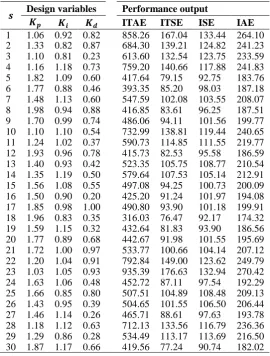
For each input computation, we run the simulation model and compute the relevant output. Total running of simulation is 𝑛𝑡 that in our case is 30 runs. Regarding Eqs.(8) to (11), four different outputs (responses) are defined for the model. In order to compare all performance creations in the same time domain, we evaluate the performance of PID controller with all creations ISE, IAE, ITSE, and ITAE in

0 ≤ 𝑡 ≤ 30 second. Table 2 represents I/O data according to each performance criteria.

Step 3. Constructing polynomial regression

(8)

Table 2. I/O data based on training sample points and each model’s performance.

Step 4. Validating metamodels with scaled residuals method

There are different approaches for validating metamodels [1]. Here, we check validation of metamodels by scaled residuals error, due to the fact that scaled residuals often give more information than other ordinary least square residuals. For this purpose, first, design 𝑛𝑣 simulation experiments (validation sample points) via LHS, then run simulation and calculate relevant outputs (𝑦𝑠) for each points (𝑠 =

1,2, … , 𝑛𝑣). So, for each input combination, compute standardized residuals as below:

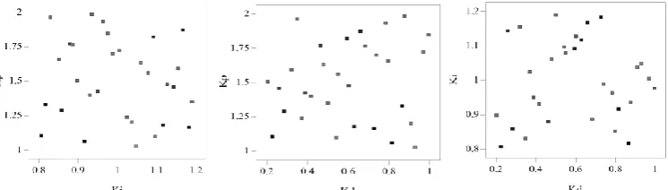
where 𝑦̂𝑠 is predicted output for 𝑠 − 𝑡ℎ input combination by metamodel that fits over training sample points. While most of the standardized residuals should be in the interval −3 ≤ 𝐷𝑠≤ 3 and any observation outside of this interval (outlier) is potentially unacceptable with respect to its observed simulation output. In the current instance, we produce 20 validate sample points. As can be seen from the scatterplots for results of validation in Fig. 6, we can accept all four metamodels because all the standardized results in each metamodel are being in [−3, +3].

𝒔 Design variables Performance output

𝑲𝒑 𝑲𝒊 𝑲𝒅 ITAE ITSE ISE IAE

1 1.06 0.92 0.82 858.26 167.04 133.44 264.10 2 1.33 0.82 0.87 684.30 139.21 124.82 241.23 3 1.10 0.81 0.23 613.60 132.54 123.75 233.59 4 1.16 1.18 0.73 759.20 140.66 117.88 241.83 5 1.82 1.09 0.60 417.64 79.15 92.75 183.76 6 1.77 0.88 0.46 393.35 85.20 98.03 187.18 7 1.48 1.13 0.60 547.59 102.08 103.55 208.07 8 1.98 0.94 0.88 416.85 83.61 96.25 187.51 9 1.70 0.99 0.74 486.06 94.11 101.56 199.77 10 1.10 1.10 0.54 732.99 138.81 119.44 240.65 11 1.24 1.02 0.37 590.73 114.85 111.55 219.77 12 1.93 0.96 0.78 415.73 82.53 95.58 186.59 13 1.40 0.93 0.42 523.35 105.75 108.77 210.54 14 1.35 1.19 0.50 579.64 107.53 105.14 212.91 15 1.56 1.08 0.55 497.08 94.25 100.73 200.09 16 1.50 0.90 0.20 425.20 91.24 101.97 194.08 17 1.85 0.98 1.00 490.80 93.90 101.18 199.91 18 1.96 0.83 0.35 316.03 76.47 92.17 174.32 19 1.59 1.15 0.32 432.64 81.83 93.90 186.56 20 1.77 0.89 0.68 442.67 91.98 101.55 195.69 21 1.72 1.00 0.97 533.77 100.66 104.14 207.12 22 1.20 1.04 0.91 792.84 149.00 123.62 249.79 23 1.03 1.05 0.93 935.39 176.63 132.94 270.42 24 1.63 1.06 0.48 452.72 87.11 97.54 192.29 25 1.66 0.85 0.80 507.51 104.89 108.48 209.13 26 1.43 0.95 0.39 504.65 101.55 106.50 206.44 27 1.46 1.14 0.26 465.71 88.61 97.63 193.78 28 1.18 1.12 0.63 712.13 133.56 116.79 236.36 29 1.29 0.86 0.28 534.49 113.17 113.69 216.50 30 1.87 1.17 0.66 419.56 77.24 90.74 182.02

𝐷𝑠=

𝑦𝑠− 𝑦̂𝑠

√1

𝑙∑𝑙𝑠=1(𝑦𝑠− 𝑦̂𝑠)2

(9)

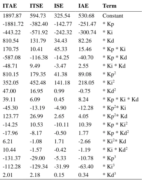
Table 3. Cubic equations of polynomial regression for all four performance creations.

Step 5. Investigate optimal solution

Search methods with less computational complexity is one of the main advantages of employing metamodels instead of an expensive original model. In such using metamodel, the common approach to searching optimal solution is the “grid search” method. In this approach, the whole design space is studied through evaluating of model components over equally spaced grid points [15, 25]. The grid points can be replaced by random points, which spread over whole design space (Monte Carlo random search) or some common space filling methods (e.g. LHS method). Here, the LHS method is used to produce search sample points. In this searching method, there is a chance to find the global optimum solution because the searching is not bounded to local “valley”. For the current case, we produce 10,000 sample points over whole design space by LHS method. Among all sample points, the optimum point is investigated when according to each metamodel, the objective is the minimization of ITAE, ITSE, ISE, and IAE. Here, the grid search method has computed the same optimum point for ITSE, ISE, and IAE. Table 4 represents the system performance, which compares two optimum points obtained by metamodels over ITAE and over ITSE, ISE, and IAE (give the same result), and by Taguchi-GRA result and tradition Ziegler-Nichols method.

ITAE ITSE ISE IAE Term

1897.87 594.73 325.54 530.68 Constant -1881.72 -382.40 -142.77 -251.47 * Kp -443.22 -571.92 -242.32 -300.74 * Ki 810.54 131.79 34.43 82.26 * Kd 170.75 10.41 45.33 15.46 * Kp * Ki -587.08 -116.38 -14.25 -40.70 * Kp * Kd -48.71 9.49 -3.47 2.55 * Ki * Kd 810.15 179.35 41.38 89.08 * Kp2 352.05 452.48 141.18 218.05 * Ki2 47.00 16.95 0.99 -0.75 * Kd2

(10)

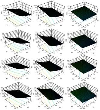
Fig. 5. Surface plots of all four metamodels over PID gain parameters (input variables).

Fig. 6. Scatterplots over standardized residuals for all four metamodels.

Design-Expert® Software Factor Coding: Actual ITAE

935.388

316.032 X1 = A: Kp X2 = B: Ki Actual Factor C: Kd = 0.6

0.8 0.9 1 1.1 1.2 1 1.2 1.4 1.6 1.8 2 200 400 600 800 1000 IT A E Kp Ki Design-Expert® Software Factor Coding: Actual ITAE

935.388

316.032 X1 = A: Kp X2 = C: Kd Actual Factor B: Ki = 1

0.2 0.4 0.6 0.8 1 1 1.2 1.4 1.6 1.8 2 200 400 600 800 1000 IT A E Kp Kd Design-Expert® Software Factor Coding: Actual ITAE

935.388

316.032 X1 = B: Ki X2 = C: Kd Actual Factor A: Kp = 1.5

0.2 0.4 0.6 0.8 1 0.8 0.9 1 1.1 1.2 200 400 600 800 1000 IT A E Ki Kd

Design-Exp ert® Software Factor Coding: Actual ITSE

176.629

0.8 0.9 1 1.1 1.2 1 1.2 1.4 1.6 1.8 2 60 80 100 120 140 160 180 200 IT SE Kp Ki

176.629

0.2 0.4 0.6 0.8 1 1 1.2 1.4 1.6 1.8 2 60 80 100 120 140 160 180 200 IT S E Kp Kd

176.629

0.2 0.4 0.6 0.8 1 0.8 0.9 1 1.1 1.2 60 80 100 120 140 160 180 200 IT SE Ki Kd

Design-Exp ert® Software Factor Coding: Actual ISE

133.436

0.8 0.9 1 1.1 1.2 1 1.2 1.4 1.6 1.8 2 80 90 100 110 120 130 140 IS E Kp Ki

133.436

0.2 0.4 0.6 0.8 1 1 1.2 1.4 1.6 1.8 2 80 90 100 110 120 130 140 IS E Kp Kd

133.436

0.2 0.4 0.6 0.8 1 0.8 0.9 1 1.1 1.2 80 90 100 110 120 130 140 IS E Ki Kd

Design-Exp ert® Software Factor Coding: Actual IAE

270.417

0.8 0.9 1 1.1 1.2 1 1.2 1.4 1.6 1.8 2 160 180 200 220 240 260 280 IA E Kp Ki

270.417

0.2 0.4 0.6 0.8 1 1 1.2 1.4 1.6 1.8 2 160 180 200 220 240 260 280 IA E Kp Kd

270.417

(11)

Table 4. Optimal points derived through different tuning methods.

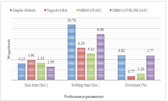
Results have confirmed the superiority of MBSO with combining polynomial regression and LHS method has compared with traditional Ziegler-Nichols method and Taguchi-GRA method. In order to reduce the computational cost, the MBSO method tries to approximate and analyze the model with a minimum number of simulation running that for the current model is equal to 30 simulation runs for training and 20 runs for validating metamodel. In the current example, the optimization model is constructed by minimizing performance criterion as a single-objective of the model (minimization of ITAE, ITSE, ISE, or IAE, separately). Results confirms that for each criterion in the presented optimal point, the single objective of the model is satisfied. The performance parameters, including rise time, settling time, and percent overshoot for all methods are shown in Fig. 7.

.

Fig. 7. Performance parameters based on MBSO method and two classic methods (Ziegler-Nichols and Taguchi-GRA).

Tuning method

Gain parameters Performance

𝑲𝒑 𝑲𝒊 𝑲𝒅 ITAE ITSE ISE IAE Rise _time (Sec.)

Settling time (Sec.)

Overshoot (%)

Ziegler-Nichols 1.59 1.00 0.63 501 97 103 203 3.21 10.70 4.82 Taguchi-GRA 2.00 0.80 0.60 349 83 96 182 3.90 6.24 0.77 MBSO (ITAE) 1.99 0.87 0.21 288 69 88 166 3.35 5.10 1.26 MBSO

(12)

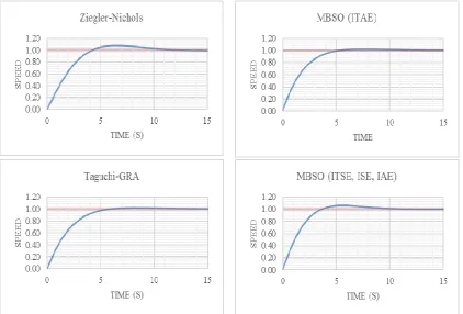
We gain the step responses of DC motor speed with PID gain parameters that respectively have obtained from traditional Ziegler-Nichols method, Taguchi-GRA, MBSO (ITAE), and MBSO (ITSE, ISE, IAE) method; see Fig. 8.

Fig. 8. Step responses with four different PID gain parameters obtain with Ziegler-Nichols, Taguchi-GRA, and MBSO.

5. Conclusion

In the current paper, the MBSO algorithm was applied for optimal design of PID controller by using hybrid polynomial regression as a metamodel and LHS method for designing of simulation experiments. Three types of sample points were produced by LHS including training points, validating points, and grid search points. The applicability and superiority of proposed method compared with two traditional Ziegler-Nichols method and Taguchi-GRA method were shown by employing practical case in PID tuning for linear speed control of DC motor. Adapting proposed method by other metamodels such as Kriging and RBF can be considered for future researches.

References

[1] Kleijnen, J. P. (2015, September). Design and analysis of simulation experiments

_:

International workshop on simulation

.

Statistics and Simulation (pp. 3-22). Springer, Cham.

[2] Huang, H. P., Jeng, J. C., Chiang, C. H., & Pan, W. (2003). A direct method for multi-loop PI/PID controller design. Journal of process control, 13(8), 769-786.

[3] Bansal, H. O., Sharma, R., & Shreeraman, P. R. (2012). PID controller tuning techniques: a review. Journal

of control engineering and technology, 2(4), 168-176.

(13)

[5] Wang, G. G., & Shan, S. (2007). Review of metamodeling techniques in support of engineering design optimization. Journal of mechanical design, 129(4), 370-380.

[6] Parnianifard, A., Azfanizam, A., Ariffin, M. K. A. M., Ismail, M. I. S., & Ale Ebrahim, N. (2018). Recent developments in metamodel based robust black-box simulation optimization: An overview. Decision science

letters, 8, (1), 17–44.

[7] Parnianifard, A., Azfanizam, A. S., Ariffin, M. K. A., & Ismail, M. I. S. (2018). Kriging-Assisted robust black-box simulation optimization in direct speed control of DC motor under uncertainty. IEEE transactions

on magnetics, 54(7), 1-10.

[8] Barton, R. R. (2009, December). Simulation optimization using metamodels. Proceedings of the 2009

wintersimulation conference (WSC) (pp. 230-238). Austin, TX, USA: IEEE.

[9] Sahraian, M., & Kodiyalam, S. (2000). Tuning PID controllers using error-integral criteria and response surfaces based optimization. Engineering optimization, 33(2), 135-152.

[10]Jiang, A., & Jutan, A. (2000). Response surface tuning methods in dynamic matrix control of a pressure tank system. Industrial & engineering chemistry research, 39(10), 3835-3843.

[11]Nakano, E., & Jutan, A. (1994). Application of response surface methodology in controller fine-tuning. ISA

transactions, 33(4), 353-366.

[12]Faucher, J. D., & Maussion, P. (2006, July). Response surface methodology for the tuning of fuzzy controller dedicated to boost rectifier with power factor correction. 2006 IEEE international symposium onindustrial

electronics (pp. 199-204). Montreal, Que., Canada

_:

IEEE.

[13]Viana, F. A. (2016). A tutorial on Latin hypercube design of experiments. Quality and reliability engineering

international, 32(5), 1975-1985.

[14]Thomas, N., & Poongodi, D. P. (2009, July). Position control of DC motor using genetic algorithm based PID controller. Proceedings of the world congress on engineering (pp. 1-3). London, UK: Newswood Limited.

[15]Li, Y. F., Ng, S. H., Xie, M., & Goh, T. N. (2010). A systematic comparison of metamodeling techniques for simulation optimization in decision support systems. Applied soft computing, 10(4), 1257-1273.

[16]Sabir, M. M., & Khan, J. A. (2014). Optimal design of PID controller for the speed control of DC motor by using metaheuristic techniques. Advances in artificial neural systems, 2014, 10.

[17]Rubaai, A., Castro-Sitiriche, M. J., & Ofoli, A. R. (2008). DSP-based laboratory implementation of hybrid fuzzy-PID controller using genetic optimization for high-performance motor drives. IEEE transactions on

industry applications, 44(6), 1977-1986.

[18]Kanojiya, R. G., & Meshram, P. M. (2012, August). Optimal tuning of PI controller for speed control of DC motor drive using particle swarm optimization. 2012 international conference on advances in power

conversion and energy technologies (APCET) (pp. 1-6). Mylavaram, Andhra Pradesh, India: IEEE.

[19]Ghany, M. A., Shamseldin, M. A., & Ghany, A. A. (2017, December). A novel fuzzy self tuning technique of single neuron PID controller for brushless DC motor. 2017 nineteenth international middle eastpower

systems conference (MEPCON) (pp. 1453-1458). Cairo, Egypt: IEEE.

[20]Dewantoro, G. (2016). Multi-objective optimization scheme for PID-controlled DC motor. International

journal of power electronics and drive systems (IJPEDS), 7(3), 734-742.

[21]Myers, R. H., Montgomery, D. C., & Anderson-Cook, C. M. (2016). Responsesurface methodology: process

and product optimization using designed experiments-fourth edittion. John Wiley & Sons.

[22]McKay, M. D., Beckman, R. J., & Conover, W. J. (1979). Comparison of three methods for selecting values of input variables in the analysis of output from a computer code. Technometrics, 21(2), 239-245.

[23]Åström, K. J., & Hägglund, T. (1995). PID controllers: Theory, design, and tuning (Vol. 2). Research Triangle Park, NC: Instrument society of America.

[24]Dellino, G., & Meloni, C. (2015). Uncertainty management in simulation-optimization of complex systems. New York: Springer.

(14)