Tsunami propagation modelling – a sensitivity study
M. H. Dao and P. Tkalich
Tropical Marine Science Institute, National University of Singapore, Singapore
Received: 23 May 2007 – Revised: 9 October 2007 – Accepted: 1 November 2007 – Published: 3 December 2007
Abstract. Indian Ocean (2004) Tsunami and following tragic consequences demonstrated lack of relevant experi-ence and preparedness among involved coastal nations. Af-ter the event, scientific and forecasting circles of affected countries have started a capacity building to tackle similar problems in the future. Different approaches have been used for tsunami propagation, such as Boussinesq and Nonlin-ear Shallow Water Equations (NSWE). These approxima-tions were obtained assuming different relevant importance of nonlinear, dispersion and spatial gradient variation phe-nomena and terms. The paper describes further development of original TUNAMI-N2 model to take into account addi-tional phenomena: astronomic tide, sea bottom friction, dis-persion, Coriolis force, and spherical curvature. The code is modified to be suitable for operational forecasting, and the resulting version (TUNAMI-N2-NUS) is verified using test cases, results of other models, and real case scenarios. Using the 2004 Tsunami event as one of the scenarios, the paper examines sensitivity of numerical solutions to variation of different phenomena and parameters, and the results are an-alyzed and ranked accordingly.
1 Introduction
Transoceanic tsunami waves have typical length of hundreds of kilometers and amplitude of less than a meter in deep oceans. Comparing with the ocean depth of a few thou-sand meters, tsunamis are classified as shallow water waves. Due to a balanced contribution of nonlinear and dispersion forces, tsunamis can propagate a long distance through an entire ocean with a little loss of energy, while bottom friction over uneven shallow ocean bathymetry may partially absorb Correspondence to: M. H. Dao
energy of the propagating waves. Additionally, astronomic tides and Coriolis force may affect tsunami dynamics.
It is important to know a comparable contribution of these and other relevant phenomena on tsunami propaga-tion. Weisz and Winter (2005) showed that the change of depth caused by tides should not be neglected in tsunami run-up calculation. Kowalik et al. (2006), Myers and Bap-tista (2001) included tide in the governing equations to in-vestigate the dynamics related to the nonlinear interaction with tide leading to amplification of tsunami height and cur-rents in the coastal region. For studying dispersive effects on tsunami wave propagation, Shuto (1991) compared numeri-cal results of three long wave theories in deep water: linear Boussinesq, Boussinesq and linear long wave. The author pointed out that linear Boussinesq and Boussinesq equations almost coincide with the true solution (given by the linear surface wave theory, which fully includes the dispersion ef-fect), suggesting that the nonlinear term is not important in the tsunami propagation in deep water. An interesting con-clusion from his study is that numerical dispersion in coarser grid made the solution better than higher-order model with the same grid length and even the same model at finer grid. Recently, Grilli et al. (2007) compared numerical results of NSWE and Boussinesq simulations for the Indian Ocean (2004) Tsunami. Their study showed a remarkable difference of surface elevation (∼20%) west of the source, in deep wa-ter. Horrillo and Kowalik (2006) did comparisons of tsunami propagation modeling using NSWE, nonlinear Boussinesq equations (NLB) and full Navier-Stokes equations aided by the Volume-Of-Fluid method (FNS-VOF). The authors con-cluded that all approaches agreed well; dispersion effect be-comes more noticeable as time advances; and NLB and FNS-VOF reproduce better small features in the leading wave. However, the computation time of NLB is much longer than NWSE, and FNS-VOF codes are even slower than NLB.
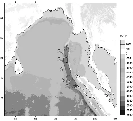
Fig. 1. Bathymetry and topography for computational domain and
the fault segments S1–S5 (?is the location of earthquake epicentre).
event. They used Manning coefficient with three different values (0.015, 0.0275 and 0.035), and a different friction pa-rameterization. Root mean square differences plotted against water depth show that most of the larger differences are oc-curred in 0–10 m depth. Significant differences are also ob-served on inundated land. The range of maximum run-up difference is from−6 to +6 m indicated that choosing fric-tion coefficient definitely influences the calculafric-tion of wave run-up on land.
The effect of Coriolis force on transoceanic tsunami was considered by Shuto (1991) and Kowalik and Murty (1989). Shuto (1991) simulated the 1969 Chilean Tsunami with and without Coriolis terms. Result shows differences in wave height but not much difference in arrival time. Kowalik and Murty (1989) concluded that the Coriolis force has a little influence on small period waves, but distinctive difference in the amplitude observed on the large period waves. They expected that tsunamis along the shelf could be modified by the Coriolis force more, because of the large period waves occurred there.
Spherical curvature of the Earth surface needs to be con-sidered in the governing equations for far-field tsunami simu-lation; however, the phenomenon was often neglected in ear-lier tsunami numerical codes.
In this paper, different modifications of well known tsunami propagation model TUNAMI-N2 (Goto et al., 1997) are developed to explore the sensitivity of the computational results to the variation of major model parameters. To take into account the Earth’s curvature in the case of propaga-tion of transoceanic tsunami, the NSWE model is formu-lated in spherical coordinates. Several other modifications are made to the original TUNAMI-N2 code in order to study
2 The tsunami model
The model TUNAMI-N2 used in this paper was originally authored by Professor Fumihiko Imamura in Disaster Con-trol Research Center in Tohoku University (Japan) through the Tsunami Inundation Modeling Exchange (TIME) pro-gram. TUNAMI-N2 is one of the key tools to study prop-agation and coastal amplification of tsunamis in relation to different initial conditions (Goto and Ogawa, 1982; Imamura and Goto, 1988; Imamura and Shuto, 1989; Goto et al., 1997, Shuto and Goto, 1988; Shuto et al., 1990). The program can compute the water surface elevation and velocities due to tsunami across entire computational domain, including shal-low and land regions. TUNAMI-N2 code was implemented to simulate tsunami propagation and run-up in Pacific, At-lantic and Indian Oceans, with zoom-in at particular areas of Japanese, Caribbean, Russian, and Mediterranean seas (Yal-ciner et al., 2000, 2001, 2002, 2004; Zahibo et al., 2003; Tinti et al., 2006).
2.1 Governing equations
TUNAMI-N2 uses second-order explicit leap-frog finite dif-ference scheme to discretize a set of NSWE. For the propa-gation of tsunami in the shallow water, the horizontal eddy turbulence terms are negligible as compared with the bottom friction. The equations are written in Cartesian coordinate (Imamura et al., 2006) as
∂η ∂t +
∂M ∂x +
∂N
∂y =0 (1)
∂M ∂t + ∂ ∂x M2 D ! + ∂ ∂y MN D
+gD∂η ∂x+
τx
ρ =0 (2)
∂N ∂t + ∂ ∂x MN D + ∂ ∂y N2 D !
+gD∂η ∂y +
τy
Fig. 2. Surface elevation for North Sumatra (December 2004) tsunami: computations vs. satellite data (Jason-1 path).
Table 1. Values of Manning’s roughness for certain types of sea bottom (Imamura et al., 2006).
Channel Material n Channel Material n
Neat cement, smooth metal 0.010 Natural channels in good condition 0.025 Rubble masonry 0.017 Natural channels with stones and weeds 0.035 Smooth earth 0.018 Very poor natural channels 0.060
HereD=h+ηis the total water depth, wherehis the still wa-ter depth andηis the sea surface elevation.MandN are the water velocity fluxes in the x- and y-directions, respectively,
M=
η Z
−h
udz=u (h+η)=uD (4)
N =
η Z
−h
vdz=v (h+η)=vD (5)
Termsτxandτy are due to the bottom friction in the x- and
y-directions, respectively, which is function of friction co-efficientf. The friction coefficient can be computed from Manning’s roughnessnby the following relationship
n=
v u u tf D
1 /3
2g (6)
Manning’s roughness is usually chosen as a constant for a given condition of sea bottom (see Table 1). For future anal-ysis it is important to note thatf increases when the total water depthDdecreases. The bottom friction terms are ex-pressed by
τx
ρ = n2
D7/3
MpM2+N2 (7)
τy
ρ = n2
D7/3
NpM2+N2 (8)
The above expression shows that the bottom friction in-creases with the fluxes, and inversely proportional to the depth. Thus wave energy dissipates faster when it propagates in shallow water areas.
2.2 Code modifications and improvements
Modern tsunami research experiences two contradictory trends, one is to include more physical phenomena (previ-ously neglected) into consideration, and another is to speed up the code to be used for the operational tsunami forecast. The optimal code for tsunami modeling supposed to be suffi-ciently accurate and fast; however, the notion of accuracy and speed is changing with time to reflect growing computational power and better understanding of tsunami physics.
The original TUNAMI-N2 model neglects Earth’s curva-ture and Coriolis force. To capcurva-ture these effects the NSWE model is reformulated as in spherical coordinates. The model is also modified to take into account dispersion terms. The equations are rewritten as
∂η ∂t +
1 Rcosφ
∂M
∂λ +
∂(Ncosφ) ∂φ
=0 (9)
∂M ∂t +
1 Rcosφ
∂ ∂λ M2 D ! + 1 R ∂ ∂φ MN D + gD Rcosφ
∂η ∂λ+
τx
ρ =(2ωsinφ) N + gD
Rcosφ ∂h ∂λ +
1 Rcosφ
∂Dψ
∂λ (10)
∂N ∂t +
1 Rcosφ
∂ ∂λ MN D + 1 R ∂ ∂φ N2 D ! +gD R ∂η ∂φ
+τy
ρ = −(2ωsinφ) M+ gD R ∂h ∂φ+ 1 R ∂Dψ ∂φ (11)
Fig. 4. Surface elevation for South Sumatra (12 September 2007) tsunami: computations vs. measurements at (a) Thai buoy “23401”, (b)
Padang tide gage.
ω=7.27×10⁻⁵rad/s, respectively. The dispersion potential function is defined as (Horrillo et al., 2006)
ψ=h 2
3 1 Rcosφ
∂2u ∂λ∂t +
1 R
∂2v ∂φ∂t
!
(12)
Neglecting the nonlinear terms and substituting the potential function into the governing equation, we obtains the Poisson equation
h2 3
1 R2cos2φ
∂2ψ ∂λ2 +
1 R2
∂2ψ ∂φ2
!
−ψ
=gh 2
3
1 R2cos2φ
∂2η
∂λ2+ 1 R2
∂2η
∂φ2
!
(13)
At every time-step, the solution of the Poisson equation gives the dispersion potential, then the Boussinesq equation is solved to get the wave field.
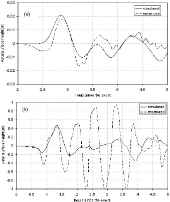
Fig. 5. Simulated sea surface elevation at Cocos Island for South Sumatra (12 September 2007) tsunami. Measurements reported: wave
amplitude 0.11 m, arrival time 1.42 h, wave period 0.37 h.
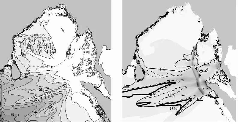
Fig. 6. Percentage difference in maximum tsunami height computed using Boussinesq and NSWE models (left – modified TUNAMI-N2,
right – FUNWAVE, Grilli et al., 2006, the same set of fault parameters are used). Dot line in the left figure is contour of 1 m wave height.
elevation term is time-centred (averaged between two time steps). Boundary condition for the Poisson equation is ob-tained via evaluation of potential function at the boundaries. To maintain stability of the solution algorithm, the time-step had to be reduced by 30%, resulting in total computational time increase by about 30% as compare to the code without dispersion term.
Using the memory accessing feature recommended in FORTRAN, all the loops in the program are optimized. The modified TUNAMI-N2 is estimated 3–4 times faster than the original code.
For easier references, in the text from here on the modified version of TUNAMI-N2 is called TUNAMI-N2-NUS, while TUNAMI-N2 is referred to the original version.
2.3 Initial and boundary conditions
The initial condition of TUNAMI-N2 is often prescribed as a static elevation of sea level due to the fault displacement (rup-ture) at the bottom. For the sub-sea earthquake, the rupture typically has duration of minutes, which can be considered as instantaneous comparing to the time-scale of tsunami prop-agation. The hydrodynamic effect is often neglected since the horizontal size of the wave profile is sufficiently larger than the water depth at the source. Thus, the initial surface wave is assumed to be identical to the vertical static coseis-mic displacement of the sea floor which is given by Masinha and Smylie (1971) for inclined strike-slip and dip-slip faults. Similar algorithm can be obtained from Okada (1985).
TUNAMI-N2-Fig. 7. Model sensitivity to astronomic tide. Differences in maximum tsunami amplitude for high and low water level (left: absolute values,
right: percentage difference).
Fig. 9. Differences in maximum tsunami amplitude computed for Manning coefficientsn=0.015 andn=0.025 (control case). Left – absolute values, right – percentage difference.
Table 2. The fault parameters for the Northern Sumatra earthquake
26 December 2004.
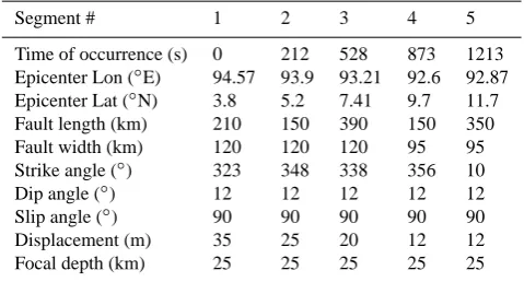
Segment # 1 2 3 4 5 Time of occurrence (s) 0 212 528 873 1213 Epicenter Lon (◦E) 94.57 93.9 93.21 92.6 92.87 Epicenter Lat (◦N) 3.8 5.2 7.41 9.7 11.7 Fault length (km) 210 150 390 150 350 Fault width (km) 120 120 120 95 95 Strike angle (◦) 323 348 338 356 10 Dip angle (◦) 12 12 12 12 12 Slip angle (◦) 90 90 90 90 90 Displacement (m) 35 25 20 12 12 Focal depth (km) 25 25 25 25 25
NUS. The fault model of Masinha and Smylie (1971) is re-peated for each individual rupture and the resulting surface deformation is linearly added to the current sea surface.
Moving boundary condition is applied for land boundaries to allow for run-up calculation, and free transmitted wave is applied at the open boundaries.
2.4 Verification of the TUNAMI-N2-NUS model
The TUNAMI-N2-NUS model is rigorously tested and ver-ified using different test cases, including hindcast of the North Sumatra event (26 December 2004) and other recent tsunamis: Taiwan (26 December 2006), Solomon Island (2 April 2007). During the event of 8.4 Mw earthquake off Bengkulu, South Sumatra (12 September 2007), the model was used in a forecast mode and provided results about 2 h after the earthquake. In this paper, we present the compar-isons of the TUNAMI-N2-NUS model to water elevation data recorded during the North Sumatra and South Suma-tra events. Bathymetry and topography for these simulations
were taken from the NGDC digital databases on a 2-min lat-itude/longitude grid (Etopo2, NGDC/NOAA).
For North Sumatra event five fault segments were assumed to rupture sequentially from south to north (Fig. 1, Table 2). Comparison to Jason-1 satellite data and some tide gages around Indian Ocean coasts are given in Figs. 2 and 3. Fig-ure 2 shows that simulated data follow very well the satellite data. First wave amplitude of 0.6 m can be hidcasted, but the second observed peak is missing in computations. At the tide gages and the yacht (Fig. 3), amplitude of the first wave is reproduced well accept at Male (Maldives). Particularly good agreement is observed at Taphaonoi. However, time lags of 6–10 min are observed at other station. Similar time lags were shown in the comparison of FUNWAVE’s result and measurement in Grilli et al. (2007).
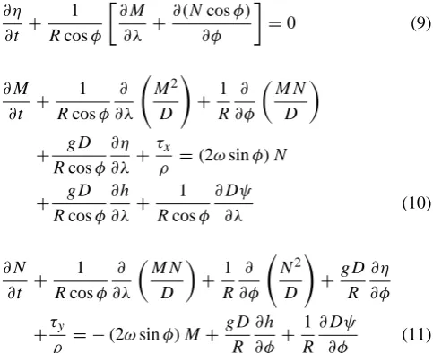
Fig. 10. Model sensitivity to friction coefficient. Surface elevation at: (a) Jason-1 path; (b) Taphaonoi (98.442, 7.801); (c) Aceh (95.309,
5.568); (d) Pulikat (80.333, 13.383).
Another verification session depicts performance of linear dispersive model mode versus fully nonlinear dispersive case for TUNAMI-N2-NUS and FUNWAVE (Grilli et al., 2006). Comparison made in Fig. 6 shows a good agreement between the two models.
3 Tsunami propagation sensitivity study
As computational power increases and more accurate nu-merical and physical approaches become available, one has
Fig. 11. Model sensitivity to Cartesian and spherical coordinates. Differences in maximum tsunami amplitude (left – absolute values, right
– percentage difference).
Fig. 13. Differences in maximum tsunami amplitude computed without and with Coriolis terms (left – absolute values, right – percentage
difference).
Fig. 14. Tsunami propagation sensitivity to Coriolis force at: (a) Jason-1 path; (b) Taphaonoi (98.442, 7.801); (c) Aceh (95.309, 5.568); (d)
Fig. 15. Differences in maximum tsunami amplitude computed with and without dispersion terms (left – absolute values, right – percentage
difference).
Fig. 16. Model sensitivity to dispersion term at: (a) Jason-1 path; (b) Taphaonoi (98.442, 7.801); (c) Aceh (95.309, 5.568); (d) Pulikat
earthquake fault parameters are given in Table 2. There were identified 5 fault segments occurred sequentially as the rup-ture propagates from south to north (Fig. 1).
3.1 Effect of tide
A typical tsunami wave is much shorter than astronomically driven tidal waves. Therefore, the tidal range was usually neglected during tsunami modeling, and the computed sea level dynamics is superimposed with the tidal one after the computations. However, in shallow areas with strong tidal activity, dynamic nonlinear interaction of tidal and tsunami waves can amplify the magnitude of inundation. To study this effect, water level change due to tide need to be included in the governing equations (Kowalik et al., 2006; Myers and Baptista, 2001).
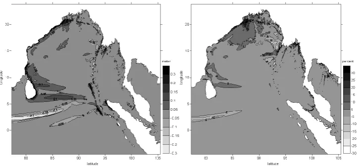
Additionally to the dynamic nonlinear interaction local-ized in inundation zones, there is a potential for a tide to change parameters of propagating tsunamis due to a simple static change of water depth by a few meters (tidal range). This effect might be important considering that a large area of the ocean may experience simultaneous elevation or sub-sidence due to the tide. For example, in the area of Thailand and Malaysia coasts, the tidal range varies roughly between −1.5 m and 1.5 m relative to the mean sea level. Thus we compare two scenarios of tsunami propagation, one occurred during low tide and another at high tide level which is 3m difference in water depth (Figs. 7 and 8). Figure 7 shows the differences in maximum tsunami amplitude between the higher and lower water depth. It can be seen that there is an extra increase of water level up to 0.7 m (or 100% wave amplitude) nearshore. Large differences present at coasts of Thailand, Malaysia, Bangladesh and west of Sri Lanka which have large area of shallow water shelf. Comparisons of tsunami height changes at deep water and tide gages are shown in Fig. 8. There is no clear difference observed along the Jason-1 path due to the water being too deep. How-ever, tsunami height can double at shallower water, such as Taphaonoi. Significant differences also present at Aceh and Pulikat. Computations show that not only the tsunami height, but arrival time could be affected by astronomical tide. One can see in Figure 8b,d that the first peak arrives∼10 min ear-lier in the computation with higher water level. Many re-searchers attributed discrepancy of tsunami computations in the near-shore zones to the bathymetry inaccuracies, but a similar error scale could be obtained by neglecting astronom-ical tides. These estimations, especially more correct
compu-ing Manncompu-ing coefficient varied with the bottom roughness. To investigate model sensitivity to variation of bottom rough-ness, Manning’s coefficient was chosen as 0.025 and 0.015 (see Table 1 for the entire range of values). The differences of computed maximum tsunami amplitude between the two sce-narios are plotted in Figs. 9 and 10, indicating that tsunami height at the lower friction can increase by 0.5 m nearshore of Malaysia, Thailand and SriLanka, however the arrival time is not affected. The friction is important only in shallow water, whereas in the deep ocean the effect is negligible.
3.3 Effect of Coriolis force and spherical coordinates Figures 11 and 12 show the model sensitivity to application of Cartesian and spherical coordinates, while Figs. 13 and 14 compare simulations with and without the Coriolis terms.
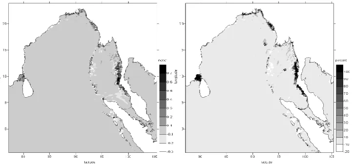
Usage of spherical coordinates may lead to a 0.3 m (or ∼30%) difference of computed maximum tsunami amplitude (Fig. 11). Although the effect of curvature is small compared to other phenomena, it is increasing at higher latitude (north-east coast of India) or farther from the source in the main direction of the tsunami propagation, such as coast of Sri Lanka. As shown in Fig. 12a, slightly change can be seen in the leading wave amplitude in deep ocean.
Governing equations indicate that Coriolis effect is ex-pected to be larger at higher latitudes or for higher current fluxes. Figure 13 particularly depicts a small variation of maximum tsunami height (10%–15%) at the northern coasts. There is no clear difference found in Fig. 14.
3.4 Effect of dispersion
Differences in maximum tsunami height between Boussinesq and NSWE approximations are presented in Figs. 15 and 16. The largest difference of maximum wave height is observed in the deep water in the main direction of tsunami wave train. Due to the frequency dispersion, longer and higher waves travel faster and separate from the shorter and smaller waves, leading to decrease of computed tsunami height. The disper-sion effect is stronger in the direction of tsunami propagation and toward deep waters where the wave speed is the largest.
events. Sensitivity analysis shown that out of the consid-ered phenomena (in order of significance), astronomic tide and bottom friction may have large impact to tsunami prop-agation in shallow waters, and thus need to be included in a research code considering wave-shore interactions. Disper-sion can leads to a notable change in amplitude of tsunami propagating a large distance in deep water; therefore, it needs to be included in trans-ocean tsunami simulation. Time re-quired to solve fully nonlinear dispersion model to gain a bit of accuracy locally, may defer the model usage for opera-tional forecast, but still may be important for run-up simula-tion. Effects of Coriolis force and spherical coordinates are smaller compared to others, but still can be used for far field tsunami modeling within the same computational resources. The final decision on when and what phenomena have to be included lays in the domain of available computational re-sources and purpose of a particular study or code. Taking into account a number of uncertainties, in operational fore-cast one might do well with the lightest (and quickest) code, whereas a research code can afford all the considered terms. Acknowledgements. This study is conducted in Tropical Marine
Science Institute (TMSI), National University of Singapore with financial support of National Environmental Agency. Help of TMSI staff is highly appreciated.
Edited by: S. Tinti
References
Etopo2, NGDC/NOAA: Surface of the Earth 2-minute color relief images, www.ngdc.noaa.gov/mgg/image/2minrelief.html, 2006. Goto, C. and Ogawa, Y.: Numerical Method of Tsunami Simula-tion with the Leap-Frog Scheme, Translated for the Time Project by Shuto, N., Disaster Control Research Center, Faculty of En-gineering, Tohoku University in June 1992, 1982.
Goto, C., Ogawa, Y., Shuto, N., and Imamura, F.: Numeri-cal method of tsunami simulation with the leap-frog scheme (IUGG/IOC Time Project), IOC Manual, UNESCO, No. 35, 1997.
Grilli, S. T., Ioualalen, M., Asavanant, J., Shi, F., Kirby, T. J., and Watts, P.: Source Constraints and Model Simulation of the De-cember 26, 2004 Indian Ocean Tsunami, ASCE J. Waterways, Port, Ocean and Coastal Engineering, 133(6), 414–428, 2007.
Kowalik, Z. and Murty, T. S.: On some future tsunamis in the Pacific Ocean, Natural Hazards, 1(4), 349–369, 1989.
Kowalik, Z. and Proshutinsky, T.: Tide-Tsunami Interactions, Sci-ence of Tsunami Hazards, Vol. 24, No. 4, p. 242, 2006. Manshinha, L. and Smylie, D. E.: The displacement fields of
in-clined faults, B. Seismol. Soc. Am., 61(5), 1433–1440, 1971. Okada, Y.: Surface deformation due to shear and tensile faults in a
half-space, B. Seismol. Soc. Am., 75, 1135–1154, 1985. Shuto, N. and Goto, C.: Numerical simulations of the transoceanic
propagation of Tsunamis, in: Sixth Congress Asian and Pacific Regional Division, International Association for Hydraulic Re-search, Kyoto, Japan, 1988.
Shuto, N., Goto, C., and Imamura, F.: Numerical simulation as a means of warning for near-field Tsunami, Coastal Engineering in Japan, 33(2), 173–193, 1990.
Shuto, N.: Numerical Simulation of Tsunamis – Its present and Near Future, Natural Hazards, 4, 171–191, 1991.
Tinti, S., Armigliato, A., Manucci, A., Pagnoni, G., Zaniboni, F., Yalciner, A. C., and Altinok, Y.: The Generating Mechanisms Of The August 17, 1999 Izmit Bay (Turkey) Tsunami: Regional (Tectonic) And Local (Mass Instabilities) Causes, Mar. Geol., 225(1–4), 311–330, 2006.
Weisz, R. and Winter, C.: Tsunami, tides and run-up: a numerical study, in: Proceedings of the International Tsunami Symposium, edited by: Papadopoulos, G. A. and Satake, K., Chania, Greece, 27–29 June 2005, 322, 2005.
Yalciner, A. C., Altinok, Y., and Synolakis, C. E.: Tsunami Waves in Izmit Bay After the Kocaeli Earthquake, Chapter 13, Kocaeli Earthquake, Earthquake Engineering Research Inst., USA, 2000. Yalciner, A. C., Synolakis, A. C., Alpar, B., Borrero, J., Altinok, Y., Imamura, F., Tinti, S., Ersoy, S., Kuran, U., Pamukcu, S., and Kanoglu, U.: Field Surveys and Modeling 1999 Izmit Tsunami, in: International Tsunami Symposium ITS 2001, Session 4, Pa-per 4–6, Seattle, 7–9 August 2001, 557–563, 2001.
Yalciner, A. C., Alpar, B., Altinok, Y., Ozbay, I., and Imamura, F.: Tsunamis in the Sea of Marmara: historical documents for the past, models for future, Mar. Geol. (Special Issue), 190, 445– 463, 2002.
Yalciner, A., Pelinovsky, E., Talipova, T., Kurkin, A., Kozelkov, A., and Zaitsev, A.: Tsunamis in the Black Sea: Comparison of the historical, instrumental, and numerical data, J. Geophys. Res., 109, C12023, doi:10.1029/2003JC002113, 2004.