Analyzing Heterogeneity In Neuroimaging With Probabilistic Multivariate Clustering Approaches

(1)

University of Pennsylvania

ScholarlyCommons

Publicly Accessible Penn Dissertations

2017

Analyzing Heterogeneity In Neuroimaging With

Probabilistic Multivariate Clustering Approaches

Aoyan Dong

University of Pennsylvania, dongaoyan@gmail.com

Follow this and additional works at:

https://repository.upenn.edu/edissertations

Part of the

Electrical and Electronics Commons

This paper is posted at ScholarlyCommons.https://repository.upenn.edu/edissertations/3041

Recommended Citation

Dong, Aoyan, "Analyzing Heterogeneity In Neuroimaging With Probabilistic Multivariate Clustering Approaches" (2017).Publicly Accessible Penn Dissertations. 3041.

(2)

Analyzing Heterogeneity In Neuroimaging With Probabilistic Multivariate

Clustering Approaches

Abstract

Automated quantitative neuroimaging analysis methods have been crucial in elucidating normal and pathological brain structure and function, and in building in vivo markers of disease and its progression. Commonly used methods can identify and precisely quantify

subtle and spatially complex imaging patterns of brain change associated with brain diseases. However, the overarching premise of these methods is that the disease group is a homogeneous entity resulting from a single, unifying pathophysiological process that has

a single imaging signature. This assumption ignores ample evidence for the heterogeneous nature of neurodegenerative diseases and neuropsychiatric disorders, resulting in incomplete or misleading descriptions. Accurate characterization of heterogeneity is important

for deepening our understanding of neurobiological processes, thus leading to improved disease diagnosis and prognosis.

In this thesis, we leveraged machine learning techniques to develop novel tools that can analyze the heterogeneity in both cross-sectional and longitudinal neuroimaging studies. Specifically, we developed a semi-supervised clustering method for characterizing

heterogeneity in cross-sectional group comparison studies, where normal and patient populations are modeled as high-dimensional point distributions, and heterogeneous disease effects are captured by estimating multiple transformations that align the two distributions, while accounting for the effect of nuisance covariates. Moreover, toward dissecting the heterogeneity in longitudinal cohorts, we proposed a method which simultaneously fits multiple population longitudinal multivariate trajectories and clusters subjects into subgroups. Longitudinal trajectories are modeled using spatiotemporally regularized cubic splines, while clustering is performed by assigning subjects to the subgroup whose population trajectory best fits their data.

The proposed tools were extensively validated using synthetic data. Importantly, they were applied to study the heterogeneity in large clinical neuroimaging cohorts. We identified four disease subtypes with distinct imaging signatures using data from Alzheimer’s

Disease Neuroimaging Initiative, and revealed two subgroups with different longitudinal patterns using data from Baltimore Longitudinal Study on Aging. Critically, we were able to further characterize the subgroups in each of the studies by performing statistical analyses

evaluating subgroup differences with additional information such as neurocognitive data. Our results

demonstrate the strength of the developed methods, and may pave the road for a broader understanding of the complexity of brain aging and Alzheimer’s disease.

(3)

Degree Name

Doctor of Philosophy (PhD)

Graduate Group

Electrical & Systems Engineering

First Advisor Christos Davatzikos

Keywords

CHIMERA, clustering, HELIOS, heterogeneity, neuroimaging

(4)

ANALYZING HETEROGENEITY IN NEUROIMAGING WITH PROBABILISTIC MULTIVARIATE CLUSTERING APPROACHES

Aoyan Dong

A DISSERTATION in

Electrical and Systems Engineering

Presented to the Faculties of the University of Pennsylvania in

Partial Fulfillment of the Requirements for the Degree of Doctor of Philosophy

2017

Supervisor of Dissertation

Dr. Christos Davatzikos

Professor of Radiology, University of Pennsylvania

Graduate Group Chairperson

Dr. Alejandro Ribeiro

Professor of Electrical and Systems Engineering, University of Pennsylvania

DISSERTATION COMMITTEE

(5)

(6)

Acknowledgments

It has been a long journey towards this thesis, six years of Ph.D. study and seven years of life in Section for Biomedical Image Analysis. I am fortunate to arrive at the end of it, with the strong support of many people along the way.

I would like to offer my sincerest gratitude to my advisor, Dr. Christos Davatzikos. It is my honor to work with him and have him as my advisor. I am grateful for his trust and support during my tenure as a graduate student. He is a great advisor, as well as a great researcher, who has carefully and patiently guided me into the beauties in science. I have learned a lot from him: critical thinking, experiment design, scientific writing, presenta-tion style, and more. Nothing in this dissertapresenta-tion would have been possible without his guidance.

(7)

of time to help me with methodology development, insightful research discussions, and papers writings, and for helping me prepare this manuscript. I would like to thank Dr. Nicolas Honnorat, who ramped me up with fundamentals of research. I am grateful to Dr. Ying Wang, Dr. Yangming Ou, and Dr. Tianhao Zhang, who shared their expertise and experiences with me during my early years of study.

My heartful thanks to Dr. Victor Preciado and Dr. Russell T. Shinohara for being on my dissertation committee and for their meaningful feedback on my work. I would also thank Dr. Shinohara for the advising and collaboration in my research.

The time spent at Penn is colorful with all my friends meet here. I would especially thank Erdem Varol, Harini Eavani and Ke Zeng for their accompany for more than five years as graduate fellows. I would thank Paraskevi Parmpi and Amanda Shacklett who provided me the convenience and support for every administrative issue. I would also like to thank all my colleagues, Aziz Ismail, Bilwaj Gaonkar, Birkan Tunc, Chunming Li, Drew Parker, Guray Erus, Hamed Akbari, Houwei Cao, Jia Wu, Jimit Doshi, Jingjing Gao, Jon Toledo, Kayhan Batmanghelich, Maria Peifer, Mark Bergman, Martin Rozycki, Meng-Kang Hsieh, Mohamad Habes, Sarthak Pati, Shandong Wu, Spyridon Bakas, Weiwei Zhang, and Xiao Da. I appreciate not only the inspirations in research but also the supporting of my life from all of them.

(8)

ABSTRACT

ANALYZING HETEROGENEITY IN NEUROIMAGING WITH PROBABILISTIC MULTIVARIATE CLUSTERING APPROACHES

Aoyan Dong Christos Davatzikos

Automated quantitative neuroimaging analysis methods have been crucial in elucidat-ing normal and pathological brain structure and function, and in buildelucidat-ing in vivo markers of disease and its progression. Commonly used methods can identify and precisely quan-tify subtle and spatially complex imaging patterns of brain change associated with brain diseases. However, the overarching premise of these methods is that the disease group is a homogeneous entity resulting from a single, unifying pathophysiological process that has a single imaging signature. This assumption ignores ample evidence for the heterogeneous nature of neurodegenerative diseases and neuropsychiatric disorders, resulting in incom-plete or misleading descriptions. Accurate characterization of heterogeneity is important for deepening our understanding of neurobiological processes, thus leading to improved disease diagnosis and prognosis.

(9)

the heterogeneity in longitudinal cohorts, we proposed a method which simultaneously fits multiple population longitudinal multivariate trajectories and clusters subjects into subgroups. Longitudinal trajectories are modeled using spatiotemporally regularized cu-bic splines, while clustering is performed by assigning subjects to the subgroup whose population trajectory best fits their data.

(10)

List of Tables

2.1 Notation used in M-step. . . 22

3.1 Cluster demographics and characteristics of CSF biomarkers and cognitive scores. . . 45

3.2 Longitudinal neuropsychological associations of the clusters. . . 50

3.3 Regression coefficients and p-values of studying longitudinal associations of cognitive measures with aHV quartiles (Quartile 1 corresponds to the lowest volume, whereas Quartile 4 is the highest). . . 52

3.4 Summary of characteristics of clusters. . . 55

4.1 Longitudinal cognitive score difference between two subgroups . . . 87

B.1 Names of 80 ROIs used in Chapter 3. . . 100

(14)

List of Figures

1.1 (A) Schema of analyzing group difference to find disease effects. (B) Under-lying heterogeneity of disease effects, mixed with covariates effects. . . 5 1.2 Multi-atlas region of interest segmentation flowchart. . . 10

2.1 (A) The problem setting:Xis the reference distribution andYis the patient distribution. (B) Our model assumption: X is transformed into a distribu-tionX0, covering the distributionY, by a set ofKdifferent transformations. 15 2.2 Atrophy patterns introduced (in red). . . 26 2.3 Simulated age effect on the normalized total volume. As age increases, the

total volume linearly decreases and the variance of the ROI volumes increases. 27 2.4 Box plot of dice scores on synthetic data between ground truth labels and

(15)

2.5 Box plot of dice scores on dementia dataset between ground truth labels and outputs of clustering methods: (a) K-means, (b) K-means with pro-file, (c) Hierarchical clustering, (d) Hierarchical clustering with propro-file, (e) CHIMERA-affine, (f) CHIMERA-duo, and (g) CHIMERA-trans. . . 31

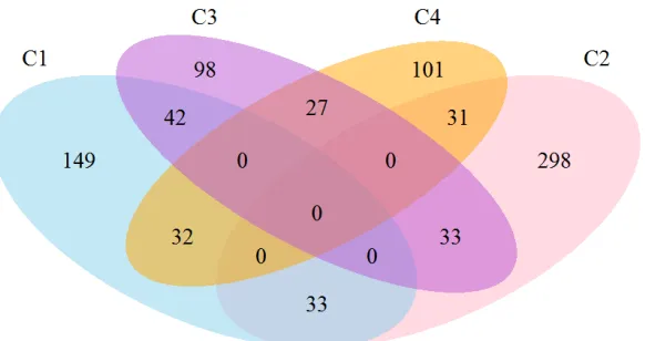
3.1 Cluster probabilities for subjects classified within each cluster. The vertical red line indicates a 0.5 probability of belonging to the cluster. . . 43 3.2 Venn diagram depicting the number of subjects classified tightly or loosely

into each cluster. Subjects with a probability>0.5 were included within a single cluster, whereas subjects with a highest cluster probability<0.5 are depicted in the interphase of the two top clusters. . . 44 3.3 VBM between the identified clusters and the CN reference group for the

ADNI-1 (A) and ADNI-GO/2 cohorts (B). Color scale represents the effect size of gray matter RAVENS maps of each comparison between a cluster and CN individuals. Red indicates greater atrophy (lower volume). Effect size maps are thresholded at false discovery rate (FDR) adjusted p-value of 0.05. . . 47 3.4 VBM between clinical groups (MCI and AD) and CN reference group in the

(16)

3.5 VBM between patient clusters, stratified by adjusted hippocampal volumes, and CN reference group in the ADNI-1 (A) and ADNI-GO/2 cohorts (B). Color scale represents the effect size of gray matter RAVENS maps of each comparison between a cluster and CN individuals. Red indicates greater atrophy (lower volume). Effect size maps are thresholded at false discovery rate (FDR) adjusted p-value of 0.05. Quartile 1 represents the lowest volume, whereas Quartile 4 is the highest. . . 49 3.6 (A) Progression from MCI to AD stratified by MRI-defined clusters. (B)

Pro-gression from MCI to AD based on aHV quartiles. Quartile 1 represents lowest volume, whereas Quartile 4 is the highest. . . 50 3.7 Longitudinal cognitive changes in ADAS-Cog13, memory and executive

composite scores in MCI subjects stratified by MRI-defined clusters. . . 51 3.8 Standardized yearly MRI changes observed in CN subjects and MCI subjects

belonging to the four identified clusters. A total of 124 CN, 57 Cluster 1, 44 Cluster 2, 18 Cluster 3 and 40 Cluster 4 subjects were included in the analysis in ADNI-1 (A). 84 CN, 15 Cluster 1, 17 Cluster 2, 17 Cluster 3 and 13 Cluster 4 subjects were included in the analysis in ADNI-GO/2 (B). . . 53 3.9 Prevalence of clusters as a function of age. (A) number of subjects with

5-year brackets, (B) relative frequency of clusters, fitted with cubic splines. . . 54 3.10 Cognitive longitudinal changes based on aHV quartiles. Quartile 1

(17)

4.1 HELIOS takes as input a longitudinal dataset (illustrated in (a) by coloring all time points of one subject the same), a set of uniform cubic B-spline bases spanning the entire time range (shown in (b)), and the number of subgroups (K=2 here). Given these, HELIOS operates by simultaneously (c) estimating the subgroup-specific global trajectories as an optimal linear combination of the four bases, and (d) assigning each subject to the global trajectory that is most similar to it. The similarity is evaluated after accounting for differences in the vertical direction through the use of offset variableD. At the end of the algorithm, clustering and fitting for all subjects with respect to the two global trajectories has been performed ((e) and (f), respectively). . . 68 4.2 Illustration of the coefficient tensorC.Cpkdenotes the coefficient vector for

a single spline; theCb_p cross section containsK sets of coefficients; theCe_k

cross section containsP sets of coefficients. . . 70 4.3 Illustration of the least squares fit: all features of the same subject share basis

B(ti), but have different coefficients fromCthat are chosen by the indicator

ζ_i. To ease the illustration, the offset variableDhas not been included here. 72 4.4 (A) The three simulated trajectory patterns. (B) Construction of four

sub-groups following different multivariate patterns, where each subject has five features. The color of each feature indicates the trajectory it follows. . . 77 4.5 Comparison between the proposed method and the two k-means variants

(18)

4.6 Comparison between the proposed method and the two k-means variants on simulated data. The performance is quantified by the adjusted rand in-dex, where results are obtained for different signal to noise ration levels, while fixing the individual trajectories length to be equal to 70% of the time range. . . 79 4.7 Distribution of scans per person by sex across the study age span. Each

point denotes a scan; horizontal lines connect scans from the same individ-ual. Red, female; blue, male. . . 81 4.8 Clustering performance measured by (A) the Adjusted rand index, and (B)

the Dunn index, for different sets of hyperparametersK andη. . . 83 4.9 Estimated trajectories for six different ROIs. The two identified subgroups

are colored red (N=29) and blue (N=73), respectively. Subgroup trajectories are thick, while the trajectories for each participant are thin. . . 85 4.10 The brain regions that follow statistically significant (FDR corrected p value

< 0.01) different trajectories between the two estimated subgroups found are shown. Red indicates G1 has a faster shrinking rate than G2, while blue indicates G1 has a faster expansion rate than G2. . . 86

(19)

Chapter 1 Introduction

1.1 Overview

Over recent years, the advances in neuroimaging have enabled massive quantitative in-vestigations of human brains, under normal and pathological conditions, and across the human lifespan. The in vivo and non-invasive multi-modal brain mapping techniques provide us with a wide array of tools of studying distinct aspects of brain structure and function. To name a few, structural magnetic resonance imaging (sMRI) reveals high-resolution brain anatomy for quantitative analysis of structural changes [85]; functional magnetic resonance imaging (fMRI) helps to measure brain activity by detecting changes associated with blood flow [138, 143]; and diffusion tensor imaging (DTI) makes it possible to understand the properties of the brain’s white matter tracts [8].

(20)

studies that aim to characterize the imaging pattern associated with a disease or a norma-tive process are designed. For example, the Alzheimer’s Disease Neuroimaging Initianorma-tive (ADNI) cohort collects patients and elderly control subjects for the sake of learning the pathological process of early Alzheimer’s disease; the Human Connectome Project (HCP) recruits healthy young adults in order to gain knowledge of the neural pathways that un-derlie brain function and behavior.

With imaging data acquired with different aims, a large amount of research put their emphasis on one common problem: discovering regionally specific effects of brain pro-cesses by proposing various analytic tools and conducting experiments on different datasets. The variations of this problem are refined in a wide range of applications: by comparing a group of patients and healthy controls, the pathological effect of brain disease can be de-lineated; by observing normal subjects across a wide spectrum of age, the normative aging effect can be quantified; by differentiating typical and non-typical developed adolescents, aberrations from normal brain development, potentially leading to neuropsychiatric dis-orders, can be better understood.

(21)

tis-The generation of tissue density maps is robust to small registration errors, which makes VBM perhaps the most popular method in population neuroimaging analysis.

However, the univariate analysis performs statistical tests on a voxel by voxel, or re-gion by rere-gion basis. Thus, these methods ignore multivariate relations between brain regions that may best characterize population differences. Instead, multivariate pattern analysis (MVPA) methods [7, 101] take advantage of dependencies among brain regions which leads to increased sensitivity. The MVPA methods can be further grouped into su-pervised and unsusu-pervised learning approaches. 1) Susu-pervised learning constitutes a set of algorithms that produce hypotheses from instances with known labeling (e.g. diagnosis, group membership), and make predictions about future instances. The supervised learn-ing methods search for multivariate imaglearn-ing patterns associated with the effect of interest. One of the most widely used methods is support vector machine (SVM) [22], which at-tempts to maximize the separation margin for different populations, that has been applied to multiple brain disease classifications [84, 87, 156]. 2) Unsupervised learning focuses on uncovering the latent structure of the imaging data. For example, principal component analysis (PCA) [1] and independent component analysis (ICA) [70] extract multivariate imaging signatures that can best explain the data variation, and are often applied to func-tional imaging [11, 49, 64]; clustering methods find subgroups of individuals with different imaging profiles [110, 115].

(22)

However, ample evidence has highlighted the heterogeneity of pathological phenotypes presented by many diseases, such as Alzheimer’s disease [90, 110], Schizophrenia [43, 86, 113], Autism spectrum disorder [78, 145], and Attention-deficit hyperactivity disor-der [158]. As a consequence, current approaches miss crucial information when describing diseases effects. By neglecting heterogeneity, these approaches can only find differences in the central tendency, such as a common imaging pattern of difference when compar-ing two populations, or an average trend of brain changes when modelcompar-ing longitudinal imaging trajectories. The brain patterns described are therefore incomplete and can be misleading in the worst case.

There exist two types of approaches for analyzing the heterogeneity in neuroimaging. 1)The first group of methods uses a priori defined neuropathological categories to iden-tify subgroups of subjects [77, 90, 110, 139]. 2) The second group comprises unbiased data-driven approaches to identify different patterns of pathology distribution based on the atrophy patterns inherent to the population [114, 115, 154]. However, in the former approaches, a priori definition of disease subtypes may be difficult to obtain (may need autopsies for neuropathological findings), or might be quite noisy and non-specific (e.g., cognitive or clinical evaluations). In the latter approaches, standard unsupervised cluster-ing methods are used to group patients along the direction associated with the largest data variability, which may not be induced by the pathology, and it might conversely reflect effects such as age, gender or disease stage.

(23)

Figure 1.1: (A) Schema of analyzing group difference to find disease effects. (B) Underlying heterogeneity of disease effects, mixed with covariates effects.

diseases can be significantly improved, and the findings can be utilized later in improv-ing disease prognosis, precision medicine and patient recruitimprov-ing for more targeted clinical trials [83, 119].

1.2 Contributions

Towards tackling the above limitations, we proposed two unbiased data-driven approaches that explicitly take into account heterogeneity in cross-sectional and longitudinal studies, respectively. In summary, this work makes the following major contributions.

(24)

cross-sectional studies as illustrated in Figure 1.1. Instead of directly finding sub-groups using standard clustering methods, we utilized information from healthy controls to guide the clustering, by assuming the probability distribution of patients is derived via a number of transformations of the probability distribution of healthy controls. These transformations define imaging signatures of heterogeneous dis-ease processes. Viewed differently, our approach clusters differences between two datasets instead of clustering data itself. This proposed paradigm has two advan-tages. First, compared to previous work [53], which produces clustering results on the subject level and thus suffers from various uninteresting variations due to the co-variates, the employed distribution matching scheme herein generates clustering on the distribution level that helps reduce the influence of population variation signifi-cantly. Second, the probabilistic modeling provides an intrinsic kernelized distance metric, which allows measuring the similarity between subjects nonlinearly. Thus, covariate effects that are often removed by an explicit linear regression step [100], can now be taken into account in a generic and nonlinear way.

(25)

diseases.

• We extended the heterogeneity analysis to tackle longitudinal designs, where we proposed HELIOS (parsing the heterogeneity of longitudinal imaging through inte-grated clustering and spatiotemporally regularized spline curve fitting). To the best of our knowledge, it is the first study that focuses on heterogeneous longitudinal tra-jectories of multivariate imaging measures. The proposed method clusters individ-ual trajectories aiming to find multiple global trajectories that can best describe the brain change across the full age range of interest of the population. The trajectories are modeled using spatiotemporal regularized splines, which 1) produces smooth and nonlinear curves in the temporal domain; 2) introduces a biological prior to the modeling. This method can be viewed as an enhanced version of linear-mixed effect models with clustering on top.

1.3 Image preprocessing

Neuroimaging data obtained from the scanner cannot be used for our analysis directly. In this section, we describe the datasets and the image preprocessing steps that were used in all of our experiments.

1.3.1 Datasets

Alzheimer’s Disease Neuroimaging Initiative (ADNI)

The Alzheimer’s Disease Neuroimaging Initiative (ADNI)1is an ongoing multicenter study designed to develop clinical, imaging, genetic, and biochemical biomarkers for the early

(26)

detection and tracking of Alzheimer’s disease (AD). The initial phase of ADNI (ADNI-1) started in 2004, with $67 million funding provided by both the public and private sectors. ADNI-1 recruited 400 subjects diagnosed with mild cognitive impairment (MCI), 200 sub-jects with early AD and 200 elderly cognitive normal subsub-jects. This study was extended with ADNI-GO which added 200 participants identified as having early mild cognitive impairment (EMCI). In 2011, ADNI-2 began with another $67 million in funding. ADNI-2 assesses participants from the ADNI-1/ADNI-GO cohort in addition to the following new participants: 150 elderly controls, 100 EMCI, 150 LMCI (late “mild cognitive impairment”) participants and 150 mild AD patients. A subset of the data from this study is used in Chapter 3 to find Alzheimer’s disease subtypes.

Baltimore Longitudinal Study on Aging (BLSA)

(27)

1.3.2 Feature extraction from structural scans

Region of interest (ROI) volumetry

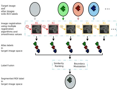
The high dimensionality of MR images hinders their analysis and interpretation. Extract-ing region of interests (ROI) effectively reduces the dimensionality of the data in an in-terpretable and anatomically meaningful way. We employed a multi-atlas segmentation algorithm [38] which uses a consensus labeling framework to fuse/integrate segmenta-tion hypotheses generated by warping a broad ensemble of labeled atlases to the target space via the use of several warping algorithms, regularization parameters, and atlases. The label fusion integrates two complementary sources of information: a local similarity ranking to select locally optimal atlases and a boundary modulation term to refine the segmentation consistently with the target image’s intensity profile. The flowchart of the ROI algorithm is presented in Figure 1.2. In our analyses, we used this algorithm to parti-tion the brain into approximately one hundred disjoint ROIs generated, and obtained the volume of each ROI as a feature representation of the brain.

Tissue density maps

(28)

Figure 1.2: Multi-atlas region of interest segmentation flowchart.

(29)

1.4 Organization of this thesis

(30)

Chapter 2 Clustering Imaging Patterns of

Disease Effect via Distribution

Matching

2.1 Introduction

(31)

Most of the group analyses assume that the members of a group share a common imag-ing pattern that differentiates them from the other group. For example, they assume that there is a unique disease effect that is found by comparing patients and controls. Such an approach can only find changes in the central tendency, i.e., a “common denominator”. However, various clinical studies have highlighted the heterogeneity of pathological phe-notypes presented by many diseases, such as Alzheimer’s disease [110, 114], schizophre-nia [43, 105], autism spectrum disorder [145], attention-deficit hyperactivity disorder [158] and cancer [54, 98]. In such cases, where we can assume that two groups differ by one pat-tern in one sub-population, and a different patpat-tern in another sub-population, a “common denominator” is at best incomplete, and at worst misleading. As a consequence, current approaches are limited in the presence of heterogeneity as they miss crucial information when modeling disease effects.

(32)

may undermine the strength of disease effect analysis.

We propose to address the aforementioned limitations by proposing a novel regular-ized clustering method based on establishing a mapping between two statistical distribu-tions. The first statistical distribution corresponds to the reference population, e.g., healthy controls, cognitive stable participants, or normally developing adolescents. The second distribution corresponds to the patient population that has been deviated from the refer-ence population under the influrefer-ence of a number of effects that we would like to describe. These effects may include heterogeneous disease processes, pathophysiological processes leading to cognitive decline, or aberrations from normal brain development. As shown in Figure 2.1, we model the heterogeneous effects as a set of transformations from the refer-ence to the patient distribution, where each transformation corresponds to one pathology subtype. The transformations are found by matching patient and reference distributions, while taking covariates such as age, sex, scanner, etc. into account (which exactly covari-ates are to be used depends highly on the specific application/study). In other words, given that a 70-year-old male Alzheimer’s disease patient would have been a 70-year-old male control had he been spared from the disease, the transition between these two states is considered to be the disease effect. This covariate-informed matching reduces the con-founding influence of the covariates, which leads to a better description of the disease effects.

(33)

(A) (B)

Figure 2.1: (A) The problem setting: X is the reference distribution andY is the patient distribution. (B) Our model assumption:Xis transformed into a distributionX0, covering the distributionY, by a set ofKdifferent transformations.

two sets of features: a set of D1-dimensional imaging features: xvm, yvn ∈ RD1; and a set ofD2-dimensional covariate features (these are known variables, such as age, sex, tumor type, treatment type):xc_m, y_nc ∈_RD2_{. For the sake of simplicity, we will denote the samples}

in the compact vector forms:xm = (xvm, xcm)andyn= (ynv, ync).

Without loss of generality, let us consider the samples as points in the imaging space (Figure 2.1). In this setting, the pathology can be viewed as the difference between Y

(34)

estimate the transformationTby matching the patient and NC distributions. The distri-bution matching paradigm consists of distance measures of imaging features, thus it is convenient to introduce covariates into the matching criteria by combining imaging and covariate-specific distances in a multi-kernel way [91].

The distribution matching problem is formulated as a maximum a posteriori (MAP) optimization problem. Thus, the optimal transformation is estimated by minimizing the following energy:

E(X,Y,Θ) =−L(X,Y,Θ) +R(Θ), (2.1)

whereΘdenotes the parameters of our model, such as transformations that are applied to

Xfor generatingY,Lis the log-likelihood of the distributionsXandYgiven the parame-ters, while a regularization/penaltyRimproves the stability/reliability of the estimation. These two parts are presented in detail in the next two sections.

2.2.1 Log-likelihood term

Due to the heterogeneity of the effects of a given disease, the pathological transition might take several directions. Therefore,Tis modeled using multiple possible transformations, where each of them represents a pathological direction of imaging change. The trans-formed NC samples are denoted as X0 = [x0₁,· · ·, x0_M], where the imaging feature xv_m is transformed toT(xv

(35)

Based on the hypothesis that the origins of patient samples are covered by the NC sam-ple space, we deduce that if we apply the pathological process model to the NC samsam-ples

X, the transformed NC point distributionX0 will cover the patient point distributionY, as shown in Figure 2.1(B).

The matching of distributions Y and X0 is found by a variant of the coherent point drift algorithm [111]. Each point x0_m is considered as a centroid of a spherical Gaussian cluster. All the clusters are assumed to have the same varianceσ2, which is inferred by the method. Points yn are treated as i.i.d. data generated by a Gaussian Mixture Model (GMM) [15] with equal weightP(x0_m) = _M1 for each cluster. The similarity between the two distribution is measured by the data likelihood of this mixture model, as presented in Equation (2.3).

In order to take covariate features into account, we adopt a multi-kernel setting. The distance between two points is measured by RBF kernels, where the kernel size of covariate features is r times larger than the kernel size of the imaging features. As a result, the likelihood of dataYgenerated by centroidsX0can be described as follows:

P(X,Y) =

N Y n=1 M X m=1

P(x0_m)P(yn|x0m)

= N Y n=1 M X m=1 1 M

rD2/2

(√2πσ)D1+D2

·exp _k

y_nv −T(xv_m)k2₊_r_k_yc

n−xcmk2

−2σ2

. (2.3)

During our experiments, the hyper-parameterrwas determined by the ratio of total vari-ance of these two features.

(36)

define the transformation for one NC point to the patient space as:

T(xv_m) =

K

X

k=1

ζkmTk(xvm). (2.4)

Ideally, if the disease subtypes were generated by distinct groups of NC points,ζkmwould be 1 for the transformation corresponding to the disease subtype that affectsxm, and value 0 otherwise. In this work, we assume that patients with different pathologies might corre-spond to the same point in the space of NC distribution, and we relax the variableζkm to sum up to 1 for eachm. This relaxation leads us to consider the transformationTfor each NC pointxmas a convex combination of all possible transformationsTk.

Linear transformation were chosen to modelTk, in order to derive analytical solutions for the distribution matching. EachTk was described by a pair of parameters(Ak, bk) ∈

(RD1×D1,RD1):

T(xv_m) =

K

X

k=1

ζkm(Akxvm+bk), (2.5)

whereP

kζkm= 1andζkm≥0for allm.

During our experiments, three different kinds ofAkmatrices were chosen: (1) full ma-trices (CHIMERA-affine), (2) diagonal mama-trices, in order to restrict the transformations to the combinations of scaling and translations (CHIMERA-duo) and (3) the identity, in order to consider only the translationsbk(CHIMERA-trans).

(37)

follow-ing expression for the log-likelihood of the data:

L(X,Y,Θ) =

N X n=1 log M X m=1 1 M

rD2/2

(√2πσ)D1+D2 exp

rkyc_n−xc_mk2 −2σ2

·exp (

ky_nv−PK

k=1ζkm(Akxvm+bk)k2

−2σ2

)

. (2.6)

2.2.2 Model regularization

As defined in the previous section, in an imaging feature space of dimension D1, the dimension of parameter space of CHIMERA-affine is in the order of O(D2₁), while for CHIMERA-duo and CHIMERA-trans is in the order ofO(D1). In the low sample size set-tings that are typically observed in medical imaging studies, this large dimension yields ill posed problems. This issue is commonly mitigated by regularizing/penalizing the pa-rameters of the transformations [41, 132]. We have adopted this approach, which improves also the generalization and the robustness of our model. In order to derive an analytical solution, we have chosen to penalize the Frobenius norm ofAk−Iand the`2 norm ofbk, whereIis the identity matrix. This regularization, is equivalent to posing Gaussian priors for the parameters.

R(Θ) = λ1

2σ2

X

k

kbkk22+ λ2

2σ2

X

k

kAk−Ik2F. (2.7)

(38)

sensi-tivity of clustering produced with respect to the individual subject variability (population variability).

2.2.3 Optimization

In this work, we have used an Expectation-Maximization algorithm [15, 108] for opti-mizing the parameters Θ = (A,b,ζ, σ2) of our model, where A = {A1,· · · , AK} and

b = {b1,· · · , bK}. The algorithm introduces latent variables z indicating the posterior probability of data pointnfor each mixture componentm,qnm=q(zn=x0m|yn). By doing so, it provides a lower bound of the log-likelihood [15]:

F0=

X

n,m

qnmlog

P(yn, x0m)

qnm

. (2.8)

The energyE is minimized via an iterative scheme. In each iterationt, the algorithm al-ternates between calculating in the E-step the expected value ofqwith respect to the pa-rameters obtained in the previous iterationΘ(t−1), and updatingΘ(t) by minimizing the objective function (Equation (2.10)) in the M-step.

During our experiments, at the initialization, the parameters σ2 was set to the mean distance between datasets X andY, ζ was set to be uniformly distributed for each xm, eachAkwas set to the identity matrixI, while the translation termbkwas sampled from a normal distributionN(0,1). The E-step and M-step were performed as follows.

E-Step:

(39)

op-timized atqnm =P(zn=x0m|yn):

qnm=

exp _k_yv

n−

P

kζkm(Akxvm+bk)k22+rkync−xcmk22

−2σ2

PM

i=1exp

_k_yv n−

P

kζki(Akxvi+bk)k22+rkync−xcik22

−2σ2

. (2.9)

M-Step:

We constructed our objective energy function F(Θ)as an upper bound of our energy functionE. The minimization ofF(Θ)leads to the minimization ofE[112]:

F(Θ) = 1

2σ2

X

m,n

qnm

kyv_n−X

k

ζkm(Akxvm+bk)k22+rkync−xcmk

2 2

+ N(D1+D2)

2 logσ

2₊ λ1

2σ2

X

k

kbkk22+ λ2

2σ2

X

k

kAk−Ik2F, (2.10)

subject to

K

X

k=1

ζkm= 1form= 1, ..., M, 0≤ζkm ≤1.

(40)

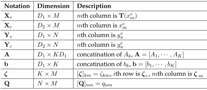
Notation Dimension Description

Xv D1×M mth column isT(xvm)

Xc D2×M mth column isxcm

Yv D1×N nth column isynv

Yc D2×N nth column isync

A D1×KD1 concatination ofAk,A= [A1,· · · , AK]

b D1×K concatination ofbk,b= [b1,· · ·, bK]

ζ K×M [ζ]km =ζkm,ith row isζi·,mth column isζ·m

Q N×M [Q]nm=qnm

Table 2.1: Notation used in M-step.

1. Updateσ2_{: The estimation of the variance is updated as follows:}

σ2 = h

tr(Yvd(Q1)YTv −2YvQXTv +Xvd(QT1)XTv)

+ tr(Ycd(Q1)YcT −2YcQXTc +Xcd(QT1)XTc)

+λ1

X

k

kbkk22+λ2

X

k

kAk−Ik2F

i.

N(D1+D2). (2.11)

2. UpdateA: depending on the nature of the matrix A, the following cases are dis-cerned:

• WhenAkis full matrix, letCij be the(i, j)th block ofC, andG= [G1,· · · , GK], whereCij andGi are obtained by:

Cij =Xvd(QT1)d(ζi·)d(ζj·)XTv (2.12)

Gi =λI+YQd(ζi·)XTv −Bd(QT1)d(ζi·)XTv. (2.13)

(41)

using Equation (2.14):

A=G(λI+C)−1. (2.14)

• WhenAkis a diagonal matrix: we first denoteAi =d(ai1, ..., aiD)and we will calculate alljth diagonal elements for allktogether,aj ∈ RK×1. LetWrsj be the(r, s)th element ofK×K matrixWj_{, which can be derived as:}

Wj_rs=X

m

x2_mjX

n

qnmζrmζsm. (2.15)

Letzm=Pkζkmbk, andUji be theith element ofK×1vectorUj:

Uj_i =X

m,n

qnmζim(zm−yn)jxmj. (2.16)

Then, we can obtain the update ofaj as follows:

aj = (Wj+λI)−1(λ1−Uj). (2.17)

3. Updateb:

LetVrsbe the(r, s)th element ofK×KmatrixV, andZrbe therth row ofK×D1 vectorZ, respectively:

Vrs=

X

qnmζrmζsm (2.18)

Zr=

X

m,n

qnmζrm(yvn−

X

k

(42)

Thus, we can derivebas:

bT = (λI+V)−1Z. (2.20)

4. Updateζ:

We adopted a gradient descent method for optimizingζ, and projected the obtained vector to the`1simplex in order to satisfy the sum-to-one constraint. LetHmbe the hessian for themth column ofζ, which can be obtained element wise using:

∂F ∂ζim

= 1

σ2

X

n

qnm(yvn−

X

k

ζkm(Akxvm+bk))T(−Aixvm−bi)

Hm_ij = ∂ 2_F

∂ζimζjm

= 1

σ2

X

n

qnm(Ajxvm+bj)T(Aixvm+bi). (2.21)

Given the above hessian estimate, we performed gradient descent, and projected the new vector to the`1simplex: [39].

ζnew_·_m =ζold_·_m −(Hm+µI)−1 ∂F ∂ζ·m

. (2.22)

During our experiments, we stopped iterating when the objective difference between two iterations reached a predefined tolerance, which was set to0.01. Because the EM al-gorithm only guarantees a local minimum solution, we ran the optimization several times, and we kept the solution with the lowest energy value.

(43)

2.2.4 Clustering

The coefficientsζkmcan be considered as the probability, for the NC samplexm, to undergo the transformationTk. LetP(yn|xm)be the likelihood of a patient sampleynto be associ-ated withxm. Then, the likelihood of a given patient sample,yn, to have been generated by the transformationTkcan be estimated by:

Pk(yn) =

X

m

P(yn|xm)ζkm. (2.23)

Because the posteriorsqnmare proportional toP(yn|xm), with a common denominator for eachn (Equation (2.9)), they can be used for partitioning the patient samples according to their main transformation. Thus, each patientyncan be assigned to the labelln, which corresponds to the largest likelihood:

ln= argmax

k

Pk(yn) = argmax

k

X

m

qnmζkm. (2.24)

As long as theζkmare stored, the label can be estimated for a novel datasby: (1) computing the likelihoodP(s|xm)based on the distances between the novel sample sand the trans-formed controlsX0, (2) computingPk(s), and (3) obtaining the label ls = argmaxkPk(s). This strategy was adopted for clustering clinical data during our experiments.

2.3 Experiments

(44)

Figure 2.2: Atrophy patterns introduced (in red).

Ward hierarchical clustering [160], as well as two variants of these methods, on synthetic data and a real dataset of dementia patients with known subtypes. The promising results obtained incited us to analyze a clinical dataset where the ground truth is unknown.

2.3.1 Synthetic data

Our method was first validated using synthetic data simulating the effect of age and dis-ease on brain volume. The brain was divided into 20 regions of interest (ROIs), where the atrophy was described by a normalized volume between 0 (the most serious atrophy) and 1 (largest possible ROI volume).

The simulated data was generated as follows:

1. 1000 samples were generated independently. For each sample, 20 ROI volumes were sampled randomly from a normal distribution, N(1,0.1). In addition, each sample was associated with a random age, sampled from a uniform distribution between 55 and 85.

(45)

Figure 2.3: Simulated age effect on the normalized total volume. As age increases, the total volume linearly decreases and the variance of the ROI volumes increases.

tionN(0.01(t−55),0.005(t−55)), wheretis the age. This simulation corresponds to a linear volume decrease with age (slope) equal to 0.01 per year; and a variance increase of slope equal to 0.005 per year.

(46)

4. The ROIs volumes were then normalized independently, by scaling them between 0 (the most atrophied sample ROI volume) and 1 (the largest sample ROI volume).

The simulated data with heteroscedastic age effect is plotted in Figure 2.3. For both groups, the normalized total volume decreases as age increases. The patient group has smaller total volume due to the disease effect. However as the variance increases, the disease effect is overwhelmed by the age effect.

We compared our model with K-means [97] clustering and Ward hierarchical cluster-ing [160]. However, standard clustercluster-ing methods do not have access to the information of control group as CHIMERA does. For a fair comparison, we considered therefore two sup-plementary variants of these clustering methods. Similar to pattern-based morphometry [53], we computed a “profile” for each patient subject. That is, we computed the difference vector between each patient point and its nearest neighbor in the control group according to the Euclidean distance between features. These profiles were clustered instead of the original patient data. In these analysis, a general linear regression (GLM) [100] was per-formed on the imaging features in order to remove the age effects prior to the clustering. The three variants of our method were applied to the synthetic data. We set model parame-ters as follows, CHIMERA-affine:(λ1, λ2) = (10,100); CHIMERA-duo:(λ1, λ2) = (10,10); and CHIMERA-trans:λ1 = 10.

(47)

Figure 2.4: Box plot of dice scores on synthetic data between ground truth labels and out-puts of clustering methods: (a) K-means, (b) K-means with profile, (c) Hierarchical cluster-ing, (d) Hierarchical clustering with profile, (e) CHIMERA-affine, (f) CHIMERA-duo, and (g) CHIMERA-trans.

based variations. CHIMERA-duo outperformed the other CHIMERA variants. This result indicates that CHIMERA-duo model contains enough degrees of freedom for capturing the differences between patient and control groups, which cannot be expressed as a pure translation. At the same time, the model is much smaller than the affine model, which is hard to regularize.

2.3.2 Neurodegenerative disease data

(48)

dis-eases generating distinct imaging patterns. We used a dementia clinical dataset of 317 T1 structural MRI scans corresponding to 148 Alzheimer’s Disease (AD) patients, 91 Parkin-son’s Disease (PD) patients and 78 Normal Controls (NC). The images were skull-stripped [37], co-registered [118] and multi-atlas ROIs were generated [38], as described in Chapter 1. We listed the names of regions used in Appendix Table B.1. The volumes of 80 ROIs were calculated, as well as the volume of brain lesions present in the data [92]. The age and gender of each subject were utilized as covariate features.

(49)

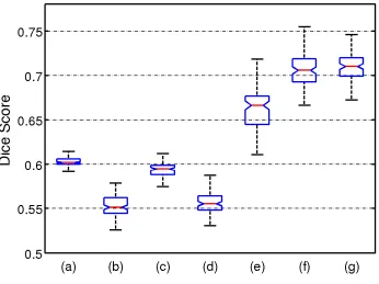
Figure 2.5: Box plot of dice scores on dementia dataset between ground truth labels and outputs of clustering methods: (a) K-means, (b) K-means with profile, (c) Hierarchical clustering, (d) Hierarchical clustering with profile, (e) affine, (f) CHIMERA-duo, and (g) CHIMERA-trans.

responding to clinically heterogeneous populations using real imaging data. Thus, we used CHIMERA to investigate the existence of disease subtypes in Alzheimer’s disease. The results of our analysis are presented in Chapter 3.

2.4 Conclusion and discussion

(50)

hetero-geneity. We discuss here three main aspects that have not been presented in detail in the previous sections. We also discuss a way to address the main limitation of our current framework.

First, the soft assignment performed by our model provides a rich information about the pathology. Each normal/control point is transformed with a probability distributionζ

by all possible transformations. This notion implies that a healthy subject might make a transition to a diseased state via various pathological patterns/processes. The clustering of patients is based on the posterior probability q andζ. Instead of a hard assignment for clustering outputs, our approach produces a probability-based soft assignment, which might better describe the disease effects.

Second, the framework is modular. In this work, we have used a linear transformation with scaling and translation that has O(D) degrees of freedom. Since the sample sizes of most neuroimaging studies are relatively small, we might improve the performance of the model by choosing a more constrained transformation. For instance, the transforma-tion could be represented by the displacement of a few reference samples [111]. Such a transformation would exhibit much fewer degrees of freedom, which could further im-prove the robustness of the optimization/clustering. Hierarchical transformations could also be implemented, similarly to [118], for reducing the computational burden and/or better constraining the transformation.

(51)

than the common approach of stratifying and matching populations based on covariates before group analyses.

(52)

Chapter 3 Capturing Heterogeneity in

Prodromal Alzheimer’s Disease

3.1 Introduction

(53)

be expected that a group of cognitively impaired subjects is composed of different sub-types. Each subtype would present a specific disease course and characteristics. While AD is not treatable, an accurate identification of the disease in its early stage could be proved crucial towards leading to more effective therapeutic interventions. Towards this end, re-search into biomarkers that can precisely quantify the subtle and complex structural and functional changes that are induced in the brain during the early stages of AD is of particu-lar interest and importance. Many studies have taken part in developing tools or applying established methodologies that use neuroimaging to improve diagnosis of AD.

Despite the increasing evidence of population heterogeneity [90, 110] and the poten-tial benefits from accurately characterizing it, most of the imaging analysis approaches ignore phenotypic heterogeneity and define patterns of structural or functional changes based on clinical categorical definitions and summarizing them with a single imaging pat-tern. On the one hand, mass univariate tools such as voxel based morphometry and its variants [6, 10, 18, 81, 82, 169] are adopted in quantifying the differences between AD pa-tients and normal control populations. On the other hand, multivariate pattern analysis [26, 42, 84, 106, 156] seeks to improve the specificity and sensitivity of computer-aided di-agnosis by encoding relations across multiple variables within a discriminative imaging pattern. However, these imaging patterns are either incomplete or worst misleading, in the presence of heterogeneity.

(54)

appropriate patient recruitment.

Recognizing the limitations of the case-control setting, previous efforts have focused on using a priori defined neuropathological categories to identify subgroups of patients [77, 90, 110, 139]. However, such neuropathological or clinical categories may not be re-liable enough for accurately distinguishing disease subtypes [93, 102]. Importantly, these approaches rely on a clinical “intuition”, thus being biased and prone to human error. Unbiased data-driven approaches show promise to be able to identify different patterns of pathology distribution based on the atrophy patterns inherent to the population [114, 115, 154]. However, commonly used standard clustering methods tend to group patients along the direction associated with the largest data variability, which may not be induced by the pathology, and which might reflect effects such as age, gender or disease stage. To avoid this, we should be steering the clustering algorithm to focus on the neurodegener-ation patterns that drive cognitive impairment. Such a clustering is more likely to lead to grouping patients into relatively homogeneous groups, with potentially more predictable clinical outcomes and treatment responses.

(55)

CN, where the patients across ADNI-1 and ADNI-GO/2 cohorts showed consistent neu-rodegenerative signatures. Subtypes in this context are mainly meant to define the main dimensions of the heterogeneity of AD, rather than imply distinct imaging phenotypes. To investigate that, we studied in detail the cerebrospinal fluid (CSF) biomarkers, cognitive characteristics and white matter hyperintensity (WMH) volumes of these subtypes.

3.2 Materials and methods

3.2.1 Subjects

A total number of 1243 AD Neuroimaging Initiative (ADNI)1participants were included in the study, including 760 ADNI-1 subjects (213 CN, 370 late MCI (LMCI), and 177 AD subjects) and 483 ADNI-GO/2 subjects (186 CN, 160 LMCI, and 137 AD). Early MCI sub-jects from the GO/2 were excluded because this group was only recruited in ADNI-GO/2. CN subjects included subjects with normal cognition, independently of the pres-ence of memory complaints. Diagnoses of MCI and AD were established as described in [103, 121, 120]. The data for this study was downloaded in December 2015. The ADNI datasets have been extensively reviewed in [161]. To evaluate differences in cognitive per-formance, we studied the previously developed memory composite score [24], the execu-tive composite score [56], and the Boston naming test scores. Median follow-up length for ADNI-1 and ADNI-GO/2 MCI subjects was 161.0 (1st quartile: 105.4 - 3rd quartile: 315.0) and 156.3 (1st quartile: 106.5 - 3rd quartile: 159.1) weeks, respectively.

(56)

3.2.2 Cerebrospinal fluid (CSF) collection and measurement

CSF samples were processed as previously described [136, 137]. Aβ1−42 and total tau (t-tau) were measured using the multiplex xMAP Luminex platform (Luminex Corp, Austin, TX) with Innogenetics (INNO-BIA AlzBio3; Ghent, Belgium; for research use-only reagents) immunoassay kitbased reagents.

3.2.3 MRI acquisition and processing

Acquisition of 1.5-T MRI (for ADNI-1) and 3.0-T MRI (for ADNI-GO/2) data at each study site followed a previously described standardized protocol that included volumetric 3D RAGE (magnetization-prepared rapid gradient-echo imaging [109]) or Sagittal MP-RAGE with variable resolution around the target of 1.2mm isotropically. The scans went through the following correction methods: gradwarp, B1 calibration, N3 correction [141], and (in-house) skull-stripping [37]. See (www.loni.usc.edu/ADNI) and [72] for details.

(57)

calculated and matched across ADNI-1 and ADNI-GO/2 cohorts using a set of matched MRIs as previously described in [155]. All the subjects were then divided into four quar-tiles in order to perform the stratification analysis based on hippocampal atrophy, which is considered to be a sensitive biomarker of dementia.

3.2.4 White matter hyperintensities (WMH)

WMH were segmented using different approaches in ADNI-1 [134] and ADNI-GO/2 [32]. The method applied on ADNI-1 utilized PD, T1, and T2 MR images. This method is based on a Bayesian Markov random field approach, where the joint posterior probability of the presence of WMH at each voxel is maximized. The posterior probability consists of a like-lihood computed from image intensities, a spatial prior that regularizes the location of WMHs, and a contextual prior that encourages neighbor voxels to have the same labels. The method applied on ADNI-GO/2 utilized FLAIR and T1 images. This method operates first by co-registering the FLAIR MR image to the T1 image, and then performing inhomo-geneity correction. The binary WMH mask is then estimated based on histogram fitting and thresholding at 3.5 standard deviations above the mean signal in brain matter distri-bution. The WMH mask is further refined by taking into account spatial prior and tissue class constraints in a Bayesian approach.

3.2.5 Heterogeneity and voxel based morphometry analysis

(58)

strengths. We took these discrepancies into account during our analyses by introducing the original recruitment cohort (ADNI-1 versus ADNI-GO/2) as a covariate in our model, in addition to age and gender. As a result, the patient and normal control distributions were matched within each cohort separately, but the pathological effects captured by CHIMERA were shared across datasets. We performed a 10-fold cross-validation using the combined dataset to evaluate the robustness of the method, which showed an 84.1% agreement. In addition, we applied our clustering approach separately in the ADNI-1 and ADNI-GO/2 cohorts, which showed a 63% and 74% overall agreement with the combined approach, respectively.

3.2.6 Statistical analysis

(59)

and time as random effects and age, gender, time, APOEε4presence and years of educa-tion as fixed effects. A Cox hazards model including age, gender, APOEε4presence and years of education as covariates, was fitted for comparing the conversion of LMCI patient to AD in the different clusters. For the evaluation of the profile of longitudinal changes in MRI volumes, individual mixed effects models that included age, gender, time and APOEε4as covariates, were applied to estimate the yearly ROI volumetric changes in CN subjects and patients belonging to the different clusters. Baseline and 2nd year MRI scans were compared for this purpose, and ROI values were standardized to compare findings across the different areas. Analyses were performed using R v. 3.2.2 [122]. The visual-ization of imaging signatures of derived clusters (i.e., the clusters found by CHIMERA), of clinically-defined (AD/MCI/AD+MCI) groups, and of aHV-defined (aHV quantiles) groups was performed via VBM [6, 23] on RAVENS maps.

3.3 Experiments and results

3.3.1 Cluster demographic and genetic characteristics

(60)

Rand Index (ARI), which indicates the reproducibility of clustering memberships, between all the pairs of the 100 clusterings obtained for each hyperparameter set, and averaged the ARI for each clustering. The hyperparameters that yielded the best reproducibility were chosen to produce clustering memberships herein.

We finally partitioned the entire set of ADNI patients into four clusters that included in each case subjects from ADNI-1 and ADNI-GO/2. Subjects in different ADNI cohorts, but within the same cluster, exhibited similar atrophy patterns. The characteristics of clus-ters identified in ADNI-1 and ADNI-GO/2 cohorts are summarized in Table 3.1. In all ADNI cohorts, Cluster 2 subjects were older and had a greater proportion of AD dementia subjects compared to Cluster 1.

3.3.2 Cluster membership confidence

In our main analysis, we assigned each subject to the cluster with the highest probabil-ity. For most of the subjects, cluster membership was assigned with a probability≥0.5. However, in the remaining cases, membership was assigned with a probability<0.5. The “tightest” cluster was Cluster 2 (87% subjects had a probability≥0.5), whereas Cluster 3 was the loosest one (66% subjects had a probability ≥0.5) (Figure 3.1), with most of the loose cases being close to Cluster 1. We summarize these findings using a Venn diagram in Figure 3.2.

3.3.3 Cross-sectional clinical and biomarker associations

(61)

(62)

(63)

Cluster 1 Cluster 2 Cluster 3 Cluster 4 P -value c C1 vs C2 C1 vs C3 C1 vs C4

Demographics ADNI-1 Number

of Subjects (%) 166 (30.35%) 213 (38.94%) 65 (11.88%) 103 (18.83%) AD (%) 34 (20.48%) 99 (46.48%) 19 (29.23%) 25 (24.27%) < 0.001 < 0.0001 0.21 0.56 LMCI (%) 132 (79.52%) 114 (53.52%) 46 (70.77%) 78 (75.73%) Age (Median a) 75.25 (69.6-79.95) 77.3 (72-81.7) 71.6 (68-76.4) 72.7 (68.55-79.9) < 0.0001 0.021 0.006 0.51 Gender (Female%) 33.13 39.91 46.15 45.63 0.13 APOE (% ε 4 pr esence) 52.41 63.85 55.38 58.25 0.15 ADNI-GO/2 Number of Subjects (%) 38 (12.79%) 131 (44.11%) 84 (28.28%) 44 (14.81%) AD (%) 9 (23.68%) 73 (55.73%) 38 (45.24%) 17 (38.64%) 0.004 < 0.001 0.039 0.23 LMCI (%) 29 (76.32%) 58 (44.27%) 46 (54.76%) 27 (61.36%) Age (Median a) 69.9 (62-74.6) 75.9 (72.15-79.9) 71.45 (64.33-77.23) 72.85 (66.28-76.43) < 0.0001 < 0.0001 0.31 0.30 Gender (Female%) 42.11 37.4 61.9 36.36 0.003 0.74 0.07 0.76 APOE (% ε 4 pr esence) 57.89 62.6 60.71 68.18 0.79 CSF biomarkers and cognitive scores

ADNI-1 Aβ

1 − 42 b(% ≤ 192pg/mL) 63.3 89.5 96.8 75.9 < 0.0001 0.0001 0.0007 0.40 T -tau 90.5 (65.5-125.2) 96 (67.75-135) 109 (86-150) 107.5 (69.75-141.8) 0.64 P-tau 31 (20.5-45) 35 (24-46.75) 38 (29-47.5) 40 (25-50.5) < 0.0001 < 0.0001 0.063 0.80 ADAS-Cog13 18.67 (14.33-22.33) 24.33 (18.67-29.67) 21 (16.17-28.41) 19.67 (16.16-24.67) < 0.0001 < 0.0001 0.0025 0.91 Memory -0.11 (-0.53-0.25) -0.59 (-0.92–0.11) -0.44 (-0.88-0.04) -0.22 (-0.55-0.1) < 0.0001 < 0.0001 0.028 0.34 Executive -0.21 (-0.75-0.49) -0.51 (-1.09-0.04) -0.25 (-1.2-0.17) 0.03 (-0.47-0.47) 0.0022 0.0097 0.52 0.66 Boston naming test 25 (22-28) 24 (21-27) 27 (23-28) 26 (22-28) 0.015 0.29 0.95 0.20 WMH 0.25 (0.11-0.71) 0.45 (0.17-1.21) 0.15 (0.06-0.42) 0.32 (0.11-0.69) 0.0022 0.0097 0.52 0.66

ADNI-GO/2 Aβ

(64)

across cohorts. Subjects in Cluster 2 and 3 included a higher frequency of subjects with pathological CSF Aβ1−42values. Cluster 2 and 3 subjects presented worse performance in the memory composite and in ADAS-Cog (Alzheimer’s Disease Assessment Scale - Cog-nitive Subscale) compared to Cluster 1. In addition, Cluster 2 subjects had worse executive composite, higher p-tau values, and greater WMH volume compared to Cluster 1 subjects. Only in ADNI-GO/2 did the clusters differ in terms of CSF t-tau values (Cluster 1 had lower values than Cluster 2 and 3).

3.3.4 Group-wise VBM results

(65)

Figure 3.3: VBM between the identified clusters and the CN reference group for the ADNI-1 (A) and ADNI-GO/2 cohorts (B). Color scale represents the effect size of gray matter RAVENS maps of each comparison between a cluster and CN individuals. Red indicates greater atrophy (lower volume). Effect size maps are thresholded at false discovery rate (FDR) adjusted p-value of 0.05.

3.3.5 Longitudinal changes

(66)

Figure 3.4: VBM between clinical groups (MCI and AD) and CN reference group in the ADNI-1 (A) and ADNI-GO/2 cohorts (B). Color scale represents the effect size of gray matter RAVENS maps of each comparison between a cluster and CN individuals. Red in-dicates greater atrophy (lower volume). Effect size maps are thresholded at false discovery rate (FDR) adjusted p-value of 0.05.

(67)

Figure 3.5: VBM between patient clusters, stratified by adjusted hippocampal volumes, and CN reference group in the ADNI-1 (A) and ADNI-GO/2 cohorts (B). Color scale rep-resents the effect size of gray matter RAVENS maps of each comparison between a cluster and CN individuals. Red indicates greater atrophy (lower volume). Effect size maps are thresholded at false discovery rate (FDR) adjusted p-value of 0.05. Quartile 1 represents the lowest volume, whereas Quartile 4 is the highest.

(68)

Cluster 1 Cluster 2 Cluster 3 Cluster 4 MCI to ADa Ref. 2.26 (<0.0001) 1.87 (0.0024) 1.27 (0.21) ADAS-Cog13 Ref. 0.20 (<0.0001) 0.09 (0.023) 0.04 (0.31) Memoryb Ref. -0.11 (<0.0001) -0.06 (0.030) 0.004 (0.86) Executiveb Ref. -0.12 (<0.0001) -0.11 (0.0005) -0.04 (0.17) Only late MCI subjects were included due to short Alzheimer’s disease (AD) subjects follow-up. Age, gender, education andAPOEwere included as covariates.

a_{Hazard ratio (P-value).}

b_{Regression coefficient (P-value).}

Table 3.2: Longitudinal neuropsychological associations of the clusters.

(A) (B)

Figure 3.6: (A) Progression from MCI to AD stratified by MRI-defined clusters. (B) Pro-gression from MCI to AD based on aHV quartiles. Quartile 1 represents lowest volume, whereas Quartile 4 is the highest.

3.3.6 Prevalence of clusters as a function of age

(69)

Figure 3.7: Longitudinal cognitive changes in ADAS-Cog13, memory and executive com-posite scores in MCI subjects stratified by MRI-defined clusters.

(70)

Quartile 1 as reference

Memory Composite Executive Composite Coefficient p-value Coefficient p-value

Quartile 1 Ref. Ref. Ref. Ref.

Quartile 2 -0.130 <0.0001 -0.122 <0.0001

Quartile 3 -0.147 <0.0001 -0.130 <0.0001

Quartile 4 -0.131 <0.0001 -0.154 <0.0001

Quartile 4 as reference

Memory Composite Executive Composite Coefficient p-value Coefficient p-value

Quartile 1 -0.016 <0.0001 0.154 <0.0001

Quartile 2 0.001 0.97 0.032 0.36

Quartile 3 0.131 0.60 0.024 0.51

Quartile 4 Ref. Ref. Ref. Ref.

Table 3.3: Regression coefficients and p-values of studying longitudinal associations of cognitive measures with aHV quartiles (Quartile 1 corresponds to the lowest volume, whereas Quartile 4 is the highest).

3.4 Discussion

(71)

(A)

(B)

(72)

Figure 3.9: Prevalence of clusters as a function of age. (A) number of subjects with 5-year brackets, (B) relative frequency of clusters, fitted with cubic splines.

cognitive decline affecting executive and memory cognitive domains. Cluster 3 showed greater cortical atrophy in parietal and dorsolateral frontal cortex with proportionately lesser involvement of the limbic cortex, compared to Cluster 2. Although Cluster 3 was as-sociated with fast cognitive decline, this decline was more marked for the executive rather than the memory composite score, which is consistent with the imaging findings. Notably, Cluster 3 MCI individuals did not show further progression to AD after four years, al-though this has to be interpreted cautiously due to the small number of subjects followed for that long a period. Finally, Cluster 4 included individuals with localized atrophy in the hippocampus and medial temporal lobe, although cognitive changes did not differ from the ones observed in Cluster 1.

(73)

pres-Neuroanatomical atrophy pattern

Alzheimer’s disease-like CSF Aβ1−42levels

Cognitive decline

Cluster 1 Mild or none; non-focal Lowest frequency Least steep Cluster 2 Widespread, greater

temporal involvement

Higher frequency Steepest for memory and executive

Cluster 3 Widespread, global Higher frequency Steepest for executive, intermediate for memory Cluster 4 Localized, temporal Lower frequency Least steep

Table 3.4: Summary of characteristics of clusters.

(74)

The variability revealed by our analysis indicates that a dimensional approach to neu-rodegeneration in cognitively impaired subjects, including MCI and AD dementia stages, is important and consistent with previous observations of atypical AD presentations [4, 25, 62, 117]. The different patterns we observed might also relate to several coincident neurodegenerative and vascular pathologies [5, 131, 150, 152].

(75)

mance of these individuals was comparable to the subjects in Cluster 1, indicating that cog-nitive summary scores might not always capture regional differences in atrophy patterns and lack the ability to detect heterogeneous atrophy patterns. Interestingly, Cluster 4 had a rather stable relative frequency as a function of age (Figure 3.9(B)), which is consistent with the interpretation of this group as newly emerging, early stage AD cases who later move into Cluster 2 as new cases take their place in Cluster 4. Longitudinal analyses are required to further test this hypothesis. Finally, Cluster 3 subjects presented predominantly execu-tive function decline and a more widespread and non-focal pattern of atrophy. Therefore, this cluster might be likely representing atypical AD presentations [117], or a mixture of pathologies, which are commonly present in demented subjects, and are associated with a relatively greater impairment of executive function [150, 152, 153, 154]. The decreasing prevalence of this group with increasing age is consistent with prior work that more “cor-tical”, or atypical presentations of AD, occur more commonly at a younger age of onset [46]. In addition, the profile of Cluster 3 is consistent with previous results indicating that hippocampal volume alone might be neither a sensitive, nor a specific biomarker in early disease stages [27, 151, 155]. This especially might be the case for atypical non-amnestic presentations without underlying AD pathology. Our results indicate that the entire pat-tern of brain atrophy needs to be taken into consideration. This also further emphasizes the potential value of such a clustering in clinical trial recruitment, as Cluster 3, similar to Cluster 2, represents a group that has a high likelihood of AD pathology based on CSF Aβ1−42levels, but in which memory and hippocampal measures would be less effective as markers of disease progression than, for example, executive measures.