https://doi.org/10.5194/dwes-11-25-2018 © Author(s) 2018. This work is distributed under the Creative Commons Attribution 4.0 License.
Mass imbalances in EPANET water-quality simulations
Michael J. Davis1, Robert Janke2, and Thomas N. Taxon3
1Argonne Associate of Seville, Environmental Science Division, Argonne National Laboratory,
Argonne, Illinois, USA
2National Homeland Security Research Center, US Environmental Protection Agency, Cincinnati, Ohio, USA 3Global Security Sciences Division, Argonne National Laboratory, Argonne, Illinois, USA
Correspondence:Michael J. Davis (mike_davis@anl.gov) and Robert Janke (janke.robert@epa.gov)
Received: 2 September 2017 – Discussion started: 26 September 2017 Revised: 22 February 2018 – Accepted: 4 March 2018 – Published: 6 April 2018
Abstract. EPANET is widely employed to simulate water quality in water distribution systems. However, in general, the time-driven simulation approach used to determine concentrations of water-quality constituents provides accurate results only for short water-quality time steps. Overly long time steps can yield errors in concentration estimates and can result in situations in which constituent mass is not conserved. The use of a time step that is sufficiently short to avoid these problems may not always be feasible. The absence of EPANET errors or warnings does not ensure conservation of mass. This paper provides examples illustrating mass imbalances and explains how such imbalances can occur because of fundamental limitations in the water-quality routing algorithm used in EPANET. In general, these limitations cannot be overcome by the use of improved water-quality modeling practices. This paper also presents a preliminary event-driven approach that conserves mass with a water-quality time step that is as long as the hydraulic time step. Results obtained using the current approach converge, or tend to converge, toward those obtained using the preliminary event-driven approach as the water-quality time step decreases. Improving the water-quality routing algorithm used in EPANET could eliminate mass imbalances and related errors in estimated concentrations. The results presented in this paper should be of value to those who perform water-quality simulations using EPANET or use the results of such simulations, including utility managers and engineers.
Copyright statement. Copyright for this publication of authors Michael J. Davis and Thomas N. Taxon is transferred to UChicago Argonne, LLC, as operator of Argonne National Laboratory, and is subject to reserved government use rights.
1 Introduction
EPANET (Rossman, 2000; US EPA, 2017a) is the standard software used for simulating water quality in a water distri-bution system (WDS). It has been widely and successfully applied for many years. The software includes a hydraulic model that determines water flow and direction throughout a network model that is used to represent a WDS. The net-work model consists of links (pipes) and nodes (junctions). The water-quality simulation is piggybacked on the hydraulic simulation. EPANET has commonly been used in situations
in which water quality does not change rapidly during the simulation. However, in some cases involving simulations of contaminant injections into a WDS it has been found that the mass of the constituent added to the network is not conserved (Davis and Janke, 2014; Davis et al., 2016). That is, at a time tin a simulation, the mass of the constituent in the network’s pipes,MP(t), and tanks,MT(t), plus the cumulative mass of
the constituent removed from the network by nodal demands, MCR(t), does not equal the cumulative mass of the
con-stituent injected into the network,MCI(t). (The mass of the
constituent in the system before the injection is zero and there is no loss of the constituent due to chemical reactions.) The mass imbalance can be large. For example, defining a mass-balance ratio (MBR) as (MP(t)+MT(t)+MCR(t))/MCI(t),
can be cases in which constituent mass is gained during a simulation (MBR>1), cases in which constituent mass is lost (MBR<1), as well as cases in which mass is conserved (MBR=1). A failure to conserve constituent mass indicates that there are errors in the estimated constituent concentra-tions, which potentially could be a concern for any appli-cation that considers water quality in a distribution system. When poor-quality network models are used, the lack of con-servation of constituent mass can be exacerbated.
EPANET is available in two forms: (1) a Microsoft
Windows® version with a user interface and (2) a
pro-grammer’s toolkit version. The latter consists of a dynamic link library of functions that allows software developers to customize their EPANET applications. The last major re-lease of EPANET, including both versions, occurred in 2000 (EPANET 2.0). The last minor release of EPANET occurred in 2008 (2.00.12). In 2012, the US EPA initiated a collab-orative, community-based open-source effort for EPANET, the “Water Distribution Network Model” project (US EPA, 2017b). In June 2015, an independent water-community-organized, open-source project began (OpenWaterAnalytics, 2017a); an open-source-project version of the EPANET pro-grammer’s toolkit (2.1) was produced in July 2016. Also in July 2016, Lewis Rossman, the original developer of EPANET, contributed a development version (EPANET 3) of the programmer’s toolkit (OpenWaterAnalytics, 2017b), which can provide mass-balance information in a status re-port after a water-quality simulation. None of the earlier ver-sions of the software provides this information.
Although versions 2.00.12 and 2.1 of EPANET do not track the mass of a water-quality constituent and its tion in a network during a simulation, both mass and its loca-tion can be determined using the concentraloca-tions of the con-stituent provided by the water-quality simulation. EPANET Example Network 3 (US EPA, 2017a) is a simple network with 97 nodes; it is called Network N1 in this paper. Con-sidering independent contaminant injections at each of the nodes in the network, Fig. 1 shows how MBRs determined for these injections are distributed after a 24 h simulation. (Details on the method used to obtain these results are pro-vided below.) The figure shows that sizable imbalances can occur in this network, unless quite small water-quality time steps are used. (EPANET’s default water-quality time step is 300 s.) These imbalances are the result of errors in the con-centrations of the constituent determined by EPANET. The water-quality routing algorithm used in EPANET does not ensure conservation of mass and large imbalances can occur because of fundamental limitations in the algorithm. Good modeling practice requires use of a water-quality time step that is less than or equal to one-tenth of the hydraulic time step, which was 3600 s for the example shown in Fig. 1. Al-though mass imbalances for all injection nodes for Network N1 can be minimized, but not eliminated, by using a water-quality time step of 60 s (one-sixtieth of the hydraulic time step), simply reducing the time step will not, in general,
en-Network N1
1 60 300 900
0.8 1 1.2 1.4 1.6 1.8
Water−quality time step (s)
Mass−balance ratio
Figure 1.Distribution of mass-balance ratios for EPANET Exam-ple Network 3 after 24 h simulations of independent contaminant injections at each network node. The horizontal black lines in the box plots give the median, the box extends from the lower to the upper quartile, and the whiskers extend to the smaller of 1.5 times the interquartile range or the most extreme data point. The hydraulic time step was 3600 s.N=94. Three nodes were excluded because there was no flow at the time the injection occurred.
sure mass conservation. In general, mass conservation cannot be ensured with the use of a nonzero water-quality time step. This paper provides examples in which mass imbalances occur, discusses why they occur, and presents a preliminary approach to water-quality modeling, currently under devel-opment for use in EPANET, which can eliminate such imbal-ances. Both the approach currently used in EPANET and the preliminary approach included in this paper use Lagrangian water-quality models: they follow individual parcels of wa-ter as they move through the network. However, the cur-rent EPANET approach uses a time-driven simulation model, while the preliminary approach presented here uses an event-driven one. The nature of time-event-driven and event-event-driven mod-els is discussed later in this paper.
2 Methods
The analysis for this paper was done with TEVA-SPOT (US EPA, 2017c), which uses a modified version of the EPANET programmer’s toolkit (2.00.12) for hydraulic and water-quality simulations in a WDS (US EPA, 2017a). The ver-sion of TEVA-SPOT used was TEVA-SPOTInstaller-2.3.2-MSXb-20170110-DEV. TEVA-SPOT was developed by US EPA’s National Homeland Security Research Center to pro-vide an ability to evaluate the consequences of intentional and unintentional releases of a contaminant into a WDS and to design contamination warning systems for a WDS. It is the only program that we are aware of that can be used eas-ily and efficiently to evaluate the consequences of injections at any or all nodes in a network model. The ability to track contaminant mass using the concentration results provided by EPANET was included in TEVA-SPOT to allow a better understanding of the distribution of a contaminant in a net-work following injection and to improve quality control for simulations. Without this capability, the failure to conserve constituent mass that can occur during EPANET simulations would not have been identified. The only significant modifi-cation made to the EPANET 2.00.12 code to support its use in TEVA-SPOT is the inclusion of the ability to allow the direct addition of contaminant mass to tanks. Any mass im-balances identified are the result of errors in constituent con-centrations provided by EPANET, not the accounting done by TEVA-SPOT.
Water-quality simulations were carried out with the time-driven water-quality model included in EPANET using four network models. Independent injection of a contaminant was simulated at all nodes in a network model (using the MASS source type in EPANET) and concentrations were deter-mined at all downstream nodes for a 168 h simulation (un-less noted otherwise). All simulations used 0.5 kg of con-taminant injected uniformly at a rate of 8.33 g min−1 over the period from 00:00 to 01:00 local time (LT), at the be-ginning of the simulation (again, unless noted otherwise). In addition, the contaminant mass in pipes and tanks and the cu-mulative mass of contaminant withdrawn from the network were determined at each reporting step in the simulation and MBRs were calculated. Contaminants were assumed to be-have as conservative tracers, with concentrations averaged over reporting intervals. Statistics on mass imbalances were determined for each network and specific injection nodes for which notable imbalances were observed were selected for evaluation of contaminant concentrations at downstream nodes. For comparison, simulations also were done for the selected injection nodes using the preliminary event-driven simulation model described here, with the same injection scenario as used with the time-driven method. The time and duration used for injections are arbitrary; however, a consis-tent injection scenario is necessary to ensure consisconsis-tent hy-draulic conditions for water-quality simulations.
Table 1.Network descriptions.
Network
Quantity N1 N2 N3 N4
Population (103) 79 5 130 250
Mean water use (m3s−1) 0.7 0.07 0.4 1.4 Per capita use (L d−1) 760 1200 280 480
Nodes (103) 0.097 1.6 6.8 13
NZD nodes (103) 0.059 0.69 6.7 11
Pipes (103) 0.12 1.4 8.0 15
Tanks 3 1 5 2
Reservoirs 2 2 1 2
Pumps 2 8 20 4
Valves 0 200 16 5
Note that all numbers are rounded independently to two significant figures. NZD: nonzero demand.
Except as noted, all simulations used a hydraulic time step of 3600 s. Various water-quality time steps were used for time-driven simulations to determine the influence of the time step on the MBR and the constituent concentrations. The default water-quality time step in EPANET is 300 s, as noted above; however, some studies, e.g., Diao et al. (2016), Helbling and VanBriesen (2009), and Wang and Harrison (2014), use substantially longer time steps. Therefore, in our analysis we include water-quality time steps longer than the default value. A reporting time step of 3600 s was used in all simulations. Event-driven simulations used a water-quality time step of 3600 s. A quality tolerance of 0.01 mg L−1was used for all simulations, except as noted.
The network models used are summarized in Table 1. Net-work N1 is EPANET Example NetNet-work 3 (US EPA, 2017a). Network N2 is a synthetic network called Micropolis (Brum-below et al., 2007). Network N3 is a model for an actual dis-tribution system that has been used in previous studies, e.g., (Davis et al., 2014). Finally, Network N4 is Network 2 in the paper “The battle of the water sensor networks (BWSN)” by (Ostfeld et al., 2008). The version of Network N4 used in this study is available; see the section below on code and data availability. No warnings or errors occurred while using EPANET with the network models and cases considered in this paper. Network schematics are provided in Appendix A.
3 Simulations with EPANET’s time-driven approach
The time-driven approach used in EPANET is discussed and examples are provided of cases in which the approach does not conserve constituent mass.
3.1 Background
not always provide exact results. In particular, if the water-quality time step is too long, concentration errors can occur; time steps should be less than the time required for a water parcel to move through the network pipe segment (link) hav-ing the shortest travel time for the simulation. In principle, errors can be avoided if a sufficiently short time step is used. However, such time steps may not be practical or feasible from a computational perspective. For example, pumps and valves have zero length in EPANET. Also, EPANET allows a minimum time step of only 1 s, which in some cases may not be sufficiently short. Finally, water parcels can move through only one link in a water-quality time step. Although relevant improvements, for example the use of parallel processing and graphics processing units (Wu, 2014), can be expected, the approach currently used in EPANET can be, and will likely remain, computationally challenging because of the possibil-ity of a large number of links in a network and the need to use a short time step to minimize concentration errors.
The algorithm used in EPANET to route water quality through a network can result in situations in which con-stituent mass is gained or lost. These imbalances can oc-cur because of the manner in which water volume and con-stituent mass are accumulated at nodes and the manner in which volume and concentration are determined for subse-quent releases to downstream links. Constituent mass can be generated during the accumulation step and lost during the release step at locations for which the volume of water being moved during a water-quality time step exceeds the volume of the link in which the water is being moved. When there is a spatial gradient in constituent concentration at such loca-tions, the mass generated during the accumulation step and lost during the release step will not be the same and a net generation or loss of constituent mass can occur. A detailed example is provided in Appendix B illustrating how the time-driven algorithm used in EPANET can fail to conserve con-stituent mass in such situations.
Restricting the movement of water parcels to only one link per water-quality time step means that, when longer time steps are used, a longer time is required for a parcel to reach a particular downstream location. For example, the arrival time of a contaminant pulse at some location following an upstream injection will be delayed if a longer time step is used. This results in concentration errors even if the shape of the pulse is unaffected. If delays are sufficiently long, the potential exists for changes in hydraulic conditions, which could also affect concentrations. Errors in concentrations due to the effects associated with allowing water parcels to move through only one link per water-quality time step can occur even if mass is conserved.
3.2 Examples illustrating mass imbalances
The examples presented in this section were obtained us-ing EPANET’s time-driven water-quality routus-ing algorithm; they demonstrate that large mass imbalances can occur, that
mass-balance and concentration results can be sensitive to the water-quality time step used, and that a very short time step may be necessary to avoid significant mass imbalances and to minimize concentration errors. These results indicate that to model contaminant intrusion events more accurately a more robust algorithm is needed for use with EPANET that can ensure conservation of mass during water-quality simu-lations.
For a contaminant injection at a selected node in Net-work N3, Fig. 2 shows how the various components of mass-balance change as the water-quality time step is varied using the time-driven simulation method in EPANET. Note that dif-ferent vertical scales are used in each plot in the figure. The mass that is injected or removed is acumulativemass; the mass in pipes and tanks is the mass in those locations at each time in the simulation. For an injection at Node 100 in Net-work N3, a significant mass imbalance can occur for water-quality time steps of 60 s or longer. At the end of the 168 h simulations, the MBRs are 7.11, 4.88, 1.38, and 1 for water-quality time steps of 900, 300, 60, and 1 s, respectively. For the time steps equal to or longer than 60 s, considerably more mass was removed from the network than was injected. A time step less than 60 s is necessary to conserve mass in this case.
Changes in MBRs following injections at Node IN1029 in Network N2 (Micropolis) are shown in Fig. 3 for the time-driven simulation method and four different water-quality time steps. Considerable time is required before the ratios stabilize for the longer time steps. Only for a time step of 1 s does the MBR approximately equal 1.0. This network contains 196 valves, which, as noted, have zero length in EPANET, and, therefore, zero travel time, which likely con-tributes to the large MBR values shown in the figure. Note in Fig. 3 that the mass imbalances are larger for a time step of 300 s than for a time step of 900 s. The location of Node IN1029 is shown in Fig. A3.
Using two different water-quality time steps, Fig. 4 shows how the MBR varies during simulations for an injection at Node JUNCTION-3064 in Network N4 (BWSN), again us-ing the time-driven method. Although the ratio stabilizes af-ter about 20 h at 1.006 for a time step of 300 s and at about 1.000 for a time step of 60 s, the ratio can be significantly different from 1.0 during the early portion of the simulations, even with a water-quality time step of 60 s. Mass is first lost from the system, then gained, then lost again, before the ratio approximately stabilizes. Note that the vertical scales on the two plots in Fig. 4 are different.
Injected Removed Pipes Tanks Time step = 900 s
MBR = 7.11
0 8 16 24 32 40 48 56 64 72 0
1 2 3
4 Time step = 300 s
MBR = 4.88
0 8 16 24 32 40 48 56 64 72 0.0
0.5 1.0 1.5 2.0 2.5
Time step = 60 s MBR = 1.38
0 8 16 24 32 40 48 56 64 72 0.0
0.1 0.2 0.3 0.4 0.5 0.6
0.7 Time step = 1 s
MBR = 1
Mass (k
g)
Time after contaminant injection (h) N3: injection at 00:00 LT at Node 100
0 8 16 24 32 40 48 56 64 72 0.0
0.1 0.2 0.3 0.4 0.5 0.6
Figure 2.Influence of the water-quality time step on the components of mass balance for an injection at Node 100 in Network N3.
Mass−balance ratio
Time after contaminant injection (h) N2: injection at 00:00 LT at Node IN1029
0 24 48
0 5 10 15 20
25 Time step (s)
900 300 60 1
Figure 3. Mass-balance ratios for injections at Node IN1029 in Network N2 during simulations with different water-quality time steps. The location of Node IN1029 is shown in Fig. A3.
reduced to 60 s. The MBRs given in the figure are values at the end of a 24 h simulation.
Contaminant concentrations at Node TN1810 in Network N2 following an injection at Node IN1029 were determined using the time-driven method and are compared in Fig. 6 for different water-quality time steps. Again, the magnitude and timing of the contaminant pulses vary with the time step used. However, in this case, rather than generally decreasing as the time step decreases, the concentration of the pulse in-creases substantially in magnitude as the time step is reduced from 900 to 300 s, consistent with the MBRs determined for this injection node and shown in Fig. 3. The maximum con-centration then decreases by over 99 % going from a time step of 300 s to a time step of 1 s. The MBRs given in the figure are values at the end of a 168 h simulation.
Time step = 300 s
0 10 20 30 40 50
0.85
0.90
0.95
1.00
Mass−balance ratio
Time step = 60 s
0 10 20 30 40 50
0.95
0.96
0.9
7
0.98
0.99
1.00
Time after contaminant injection (h) N4: injection at 00:00 LT at Node JUNCTION−3064
Figure 4.Examples of how the mass-balance ratio can vary during simulations. Results are for an injection at Node JUNCTION-3064 in Network N4. The location of Node JUNCTION-3064 is shown in Fig. A4.
of a 168 h simulation. Figure 2 shows how the components of mass balance vary following an injection at Node 100 for the same time steps used in Fig. 7.
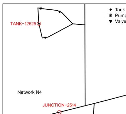
Figure 8 compares contaminant concentrations obtained for a receptor node, TANK-12525, in Network N4 follow-ing an injection at Node JUNCTION-2514, usfollow-ing different water-quality time steps. Again, the simulations used the time-driven method. In this case, the timing of changes in concentration is similar for all the time steps used and there is a high degree of correlation between the results for the different time steps. However, concentration increases con-sistently as the time step decreases, unlike the trends in the previous examples. Concentrations appear to have approxi-mately stabilized by a time step of 60 s, with little increase in concentrations occurring when the time step is reduced to 1 s. The MBRs given in the figure were determined at the end of a 168 h simulation. Note that the MBR is less than 1.0 for time steps greater than 1 s. Substantial losses of contaminant mass can occur for longer time steps.
Statistics on the extent of mass imbalance at the end of simulations that used the time-driven method are provided in Table 2 for the four networks considered. The results in the table are based on independent injections at most nodes for each of the networks. For example, the statistics for Network N4 are based on independent simulations of injections done for most of the 12 523 nodes in the network; a small fraction of the nodes were excluded, as discussed in the next para-graph. The table provides the range in MBRs determined for each network for each of four water-quality time steps and the fraction of injection nodes for which there were imbal-ances above some thresholds (e.g., 1, 5, 10 %).
MBRs equal to zero were obtained for injections at some nodes: the numerator in the MBR was zero because no mass was present in the pipes or tanks at the end of the simula-tion and no mass was removed during the simulasimula-tion. Such cases can occur when there is no flow at the time of
injec-tion (e.g., zero-demand nodes). When there is no flow at the time of injection, no contaminant mass is added to the water in the WDS and the injected mass is effectively lost, although the accounting process considers it to be mass in-jected when determining an MBR. Injection nodes for which an MBR was equal to zero at the end of a simulation were not included when determining the statistics shown in Ta-ble 2. For Network N4, two additional nodes (JUNCTION-9097 and JUNCTION-12348) also were excluded. These two nodes are in dead-end areas with no demands. Therefore, there should be no flows in these areas. However, the net-work model had a small initial flow at these nodes, inconsis-tent with a lack of demands in the dead-end areas. (EPANET determines concentrations of constituents in outflows from a node using the flow-weighted sum of inflow concentrations. If other inflows are very small, such anomalous flows could be significant in relative terms and result in concentration anomalies as well.) For Network N3, five nodes had MBRs near 0.2 for all water-quality time steps; however, when the hydraulic and reporting time steps were changed to 1 min, the MBRs for the 1 min and 1 s water-quality time steps were near 1. MBRs near 1 were used for the five nodes when de-termining the statistics for Network N3 shown in Table 2.
Table 2.Statistics for mass imbalances.
MBR Injection nodes (%) with imbalances
Network WQTS (s) Max. Min. >1 % >5 % >10 % >50 %
N1 1 1.00 1.00 0 0 0 0
60 1.02 >0.99 2 0 0 0
300 1.15 0.97 38 6 1 0
900 1.77 0.83 65 46 31 5
N2 1 1.05 0.08 2 1 1 1
60 6.49 0.06 39 29 18 5
300 23.45 <0.01 47 39 32 17
900 31.16 <0.01 52 49 44 24
N3 1 1.03 0.99 1 0 0 0
60 1.39 0.92 7 1 a 0
300 4.88 0.22 35 15 8 1
900 15.74 0.08 57 36 25 6
N4 1 1.01 0.83 b c d 0
60 1.04 0.67 1 e c 0
300 1.21 0.61 21 4 2 0
900 2.60 0.09 44 28 19 1
WQTS: water-quality time step; MBR: mass-balance ratio. Results do not include cases with MBR=0, which occurs for nodes with no flow at the time of injection. In addition, for Network N4, two nodes also are excluded that are in dead-end areas with no demands, but that have small flows at the beginning of the simulation. A total of three nodes are excluded for Network N1 (3 %), 92 or 93 for Network N2 (6 %), depending on the time step, 55 or 56 for Network N3 (1 %), again depending on the time step, and 404 for network N4 (3 %). See text for discussion.a13 nodes.b11 nodes.c2 nodes.d1 node.e3 nodes.
the sizable fraction of nodes in all the networks that have im-balances for a time step of 300 s, although the imim-balances for Networks N1 and N4 are relatively minor for this time step, with only about 1 and 2 % of nodes in these networks, respectively, having an imbalance greater than 10 %.
For a small fraction of the injection nodes in Networks N2, N3, and N4, about 0.8, 0.5, and 0.2 % of all nodes, re-spectively, the MBR did not change as the water-quality time step decreased or did not change so that the MBR converged toward 1.0. The lack of convergence of the MBR for these nodes had limited influence on the statistics in Table 2; it did influence the values shown for the minimum MBR for Network N2, particularly for a time step of 1 s. The non-convergence can be the result of several factors, including cases involving nodes in dead-end areas, as noted above. In addition, some cases had flows at the time of injection that were unexpected, given a lack of demands; the flows disap-peared for subsequent time steps. Some problems appear to be related to the hydraulic solution; these were eliminated if a short (60 s) hydraulic time step was used.
Mass balances are sensitive to the injection time used. An acceptable mass balance for a particular application for a given injection node does not guarantee an acceptable mass balance if hydraulic conditions are changed. As an example of the extreme changes that can occur when hydraulic condi-tions change, consider an injection at Node VN1263 in Net-work N2 (see location in Fig. A3), a 168 h simulation, and a 900 s water-quality time step. For a 1 h injection starting at 06:00, the MBR at the end of the simulation was 467. For
a 1 h injection starting at 00:00, the MBR at the end of the simulation was 0.007. In the first case, much more mass was removed from the network by nodal demands during the sim-ulation than was injected; in the second case, very little mass remained in the system at the end of the simulation or was removed from the system by nodal demands during the sim-ulation. In both cases the extreme values for the MBR are the result of errors in the estimated concentrations downstream from the injection location, too high in the first case and too low in the second. These errors resulted in the erroneous nu-merical generation or loss of constituent mass in the system. The cases considered to this point used relatively short, 1 h injections. However, major mass imbalances also occur for injections with long durations. For example, with a 300 s water-quality time step, the largest MBR for any injection node in Network N2 for a 1 h injection at 00:00 is about 23; for 6 and 12 h injections at that time the largest MBRs are 1495 and 971, respectively. About 17, 22, and 22 % of injec-tion nodes have mass imbalances greater than 50 % for the 1, 6, and 12 h injections, respectively. About 32, 39, and 35 % have imbalances greater than 10 %. The statistics for mass imbalance are relatively insensitive to injection duration for this network. However, mass balances for a particular injec-tion node can be sensitive to the injecinjec-tion durainjec-tion. For ex-ample, for Node VN1263 in Network N2 the MBRs are 3.3, 1495, and 971 for injections at 00:00 with durations of 1, 6, and 12 h, respectively.
imbal-0 5 10 15 20 25 0.0
0.1 0.2 0.3 0.4
Time after contaminant injection (h)
Cont
aminant concentration (mg L
−1 )
Time step (s) 900 300 60 1
MBR
1.5836 0.9996 0.9999 1.0 N1: injection at 00:00 LT at Node 101, receptor at Node 247
Figure 5.Influence of the water-quality time step on estimated con-taminant concentrations at Node 247 in Network N1 following an injection at Node 101 at 00:00 LT. Locations of the nodes are shown in Fig. A1.
80 100 120 140
0 2 4 6 8 10
Time after contaminant injection (h)
Cont
aminant concentration (mg L
−1 )
MBR 16.63 23.45 6.49 1.01 Time step (s)
900 300 60 1 N2: injection at 00:00 LT at Node IN1029,
receptor at Node TN1810
Figure 6.Influence of the water-quality time step on estimated con-taminant concentrations at Node TN1810 in Network N2 following an injection at Node IN1029 at 00:00 LT. Locations of the nodes are shown in Fig. A3.
ances. Consider a case involving chlorine decay with both bulk and wall reactions and EPANET Example Network 1 (US EPA, 2017a) with default input parameters, except for the water-quality time step. No water-quality sources were used; however, initial chlorine concentrations were specified. The network is very simple, with only 9 junctions and 12
pipes. A chlorine mass imbalance of 0.85 % (<1 %) was ob-tained for a water-quality time step of 900 s and a 24 h simu-lation. For time steps of 300, 60, and 1 s, the imbalances were 0.77, 0.58, and 0.49 %, respectively. Mass imbalance was de-termined in EPANET 3 in the same manner as discussed in this paper except that the initial mass of chlorine in the sys-tem also was considered, as was the mass of chlorine lost due to chemical reactions. Execution time increased from about 0.02 s to about 0.03, 0.04, and 1 s when the time step was de-creased from 900 s to 300, 60, and 1 s, respectively, an overall increase in execution time of about 50 fold. To obtain mass imbalances well below 0.1 %, a time step well below 1 s may be needed, along with additional increases in execution time. This is an extremely small, simple network and large im-balances are not expected. For this example, the EPANET 3 code (OpenWaterAnalytics, 2017b) was compiled using the GNU Compiler Collection (GCC, 2017).
EPANET allows four source types to be used to define lo-cations of sources of constituents (Rossman, 2000). As noted above, the simulations in this study used the MASS source type, which allows a source strength to be specified in terms of mass added per unit time. The other source types (CON-CEN, FLOWPACED, and SETPOINT) all specify source strength in terms of concentration. All are similar in that they allow the addition of the mass of some constituent to the sys-tem. EPANET’s failure to conserve constituent mass is not related to how the mass is added to the system. Therefore, the findings presented here related to a failure to conserve mass apply independently of the source type used in the sim-ulation. As the example discussed in the preceding paragraph demonstrates, failure to conserve mass can occur in situations in which no sources are used and the only mass present in the system is the result of the initial water quality specified.
4 Simulations with the preliminary event-driven approach
The preliminary event-driven approach is discussed and re-sults obtained using this approach are compared to those ob-tained using the time-driven approach.
4.1 Background
Changes in a WDS do not occur at regular time intervals. For example, the time required for a water parcel to move from node to node in the system varies from pipe to pipe and also within a pipe as conditions change. In addition, some pipes can be short, have a high flow rate, and require only a short time for a water parcel to move through them. This transit time can be too small to be practical for use as a water-quality time step in a simulation. A situation in which events (changes) occur at irregular intervals suggests use of an event-driven simulation.
EPANET using the current time-driven approach. The event-driven approach used is conceptually similar to, but was de-veloped independently of, the Lagrangian event-driven sim-ulation method discussed in (Rossman and Boulos, 1996). An event-driven method updates the state of water quality in the system only when a change (an event) occurs dur-ing the simulation, in contrast to the current time-driven method in EPANET, which updates water quality across the entire network at fixed time steps. Numerous events can occur during a time step, as water moves through the network. Various event-driven approaches have been pre-sented previously, for example by Boulos et al. (1994, 1995). The preliminary event-driven algorithm discussed here is in-cluded as an option in the current version of TEVA-SPOT (TEVA-SPOTInstaller-2.3.2-MSXb-20170110-DEV) and is being made available to EPANET developers to obtain com-munity support and assistance with improving and evaluating the algorithm.
The event-based, water-quality routing algorithm used here moves homogeneous volumes of water (water parcels with a uniform concentration of a water-quality constituent) through a network. Initially, water parcels are accumulated at all nodes where water enters the system. Nodes with ac-cumulated water parcels from all inflow links are processed in an arbitrary order. Mixing or combining of water parcels occurs at nodes based on the inflow rates of the links flow-ing into the nodes. Water parcels are combined if the abso-lute difference between their concentrations is less than some specified amount (the quality tolerance), consistent with the approach used in EPANET 2. After parcels are combined at a node, any nodal demand is removed; the remaining wa-ter parcels then are split based on the flow rates of the links flowing from the nodes. These parcels are added to lists of parcels for the downstream links. Any volume in excess of the volume of a link is removed from the leading parcels and placed at the downstream node for further processing. That node is then added to the set of nodes with accumu-lated water parcels waiting to be processed. Due to recircu-lating flows, situations can occur in which none of the nodes waiting to be processed has accumulated water parcels on all inflow links. In such cases, an incomplete parcel with the volume that will be moved, but an unspecified concentration, is created for each inflow link that does not have an accumu-lated inflow. These incomplete parcels are moved, combined, and split in the same manner as parcels for which constituent concentration has been determined; however, internal refer-ences are maintained that allow concentrations to be updated when parcels for which concentrations have been determined arrive at a node for which incomplete parcels were created. Flow reversals between hydraulic time steps are accommo-dated in the same manner as in EPANET 2. The event-driven simulation method provides results that do not depend on the water-quality time step if it is equal to or shorter than the hy-draulic time step. The method actually does not require an independent water-quality time step: the simulation is
event-driven as long as the hydraulic conditions do not change. Because by construction the method accounts for every in-dividual water parcel, its resulting MBR will always be 1.0. An example illustrating the operation of the algorithm us-ing a case with recirculatus-ing flow is provided in Appendix C. Working through the example provided in the appendix will provide a better understanding of the approach outlined in this paragraph.
4.2 Discussion
Concentrations obtained using EPANET’s time-driven al-gorithm tend to converge toward those obtained using the event-driven algorithm as the water-quality time step used in the time-driven algorithm decreases. For short water-quality time steps (e.g., 1 s) with the time-driven approach, the re-sults for the two methods can be very similar and differences can be difficult to see in the plots used in this paper. There-fore, to better examine this convergence, least-squares fits were determined relating (1) the concentrations obtained us-ing the time-driven approach with a water-quality time step of 1 s (TD1) and the concentrations obtained using the same approach with a 60 s time step (TD60), (2) TD1 and the con-centrations obtained using the time-driven approach with a 300 s time step (TD300), and (3) TD1 and the concentra-tions obtained using the event-driven approach with a 3600 s time step (ED3600). These least-squares lines have the form
ˆ
y=ax+b, whereaandbare the slope and intercept of the fitted least-squares line,xis the value of TD1, andyˆis the fit-ted value of TD60, TD300, or ED3600, depending on which is being used. The results of fitting least-squares lines are shown in Table 3 for the four cases examined in Figs. 5 to 8. The number (N) of hourly concentration values used to obtain the results shown in the Table 3 corresponds approx-imately to the number of hourly concentration values shown in the figures for the different networks. For Network N1,N was 24, covering the entire length of the simulation. For Net-work N2, it was 60, the length of the middle portion of the plot in Fig. 6. For Network N3,N was 39, the length of the period from hour 1 in the simulation to hour 40 (see Fig. 7). For Network N4, results for the entire 168 h simulation were used. The water-quality tolerance in the simulations used to obtain the concentrations needed for the analysis presented in the table was 0.01, except for the event-driven simulations for Network N4, for which 0.1 was used.
Table 3.Least-squares fits of concentration results.
Network N Case a b adj-R2 Residual SD
N1 24 TD300 0.2547 0.0074 0.0478 0.0273
TD60 0.9985 −1×10⁻⁶ 0.9999 0.0003
ED3600 0.9995 0.00001 1 0.0001
N2 60 TD300 −24.68 2.14 −0.0169 3.385
TD60 52.42 0.0334 0.3196 0.0911
ED3600 0.944 0.0003 0.7657 0.0006
N3 39 TD300 6.159 −0.0115 0.8866 0.1398
TD60 1.515 −0.00351 0.9866 0.0112
ED3600 0.9997 0.0001 0.9999 0.0005
N4 168 TD300 0.7250 0.0016 0.9956 0.0011
TD60 0.9840 0.0001 1 0.0001
ED3600 0.9791 0.0018 0.9762 0.0035
This table gives the parameters of a least-squares fit of the concentrations for the cases shown to the concentrations obtained using the time-driven algorithm with a water-quality time step of 1 s. Quantitiesa andbare the slope and intercept, respectively, of the least-squares line. Cases are TD300, the time-driven algorithm with a 300 s time step; TD60, the time-driven algorithm with a 60 s time step; and ED3600, the event-driven algorithm with a 3600 s time step.N: number of hourly concentration values used. SD: standard deviation.
0 10 20 30 40
0 1 2 3 4 5
Time after contaminant injection (h)
Cont
aminant concentration (mg L
−1 )
Time step (s) 900 300 60 1
MBR
7.11 4.88 1.38 1.00 N3: injection at 00:00 LT at Node 100,
receptor at Node 200
Figure 7.Influence of the water-quality time step on estimated con-taminant concentrations at Node 200 in Network N3 following an injection at Node 100 at 00:00 LT.
results for the time-driven approach are converging to those for the event-driven approach as the water-quality time step used for the time-driven approach decreases. For Network N4 there is a high degree of correlation between the concen-trations obtained using the time-driven method with different time steps (cf. Fig. 8) and the quality of the fit is similar for all three cases considered. However, because the magnitude of the concentrations increases as the time step decreases, the
0 50 100 150
0.00
0.02
0.04
0.06
0.08
0.1
0
Time after contaminant injection (h)
Cont
aminant concentration (mg L
−1 )
Time step (s)
900 300 60 1
MBR 0.09 0.70 0.98 1.00 N4: injection at 00:00 LT at Node JUNCTION−2514,
receptor at Node TANK−12525
Figure 8.Influence of the water-quality time step on estimated con-taminant concentrations at Node TANK-12525 in Network N4 fol-lowing an injection at Node JUNCTION-2514 at 00:00 LT. Loca-tions of the nodes are shown in Figs. A4 and A5.
slope of the least-squares line increases going from TD300 to TD60.
Table 4. Comparison of execution times for the time-driven and event-driven algorithms.
Execution time (s)
Network Injection location TDa EDb
N1 All 97 nodes 259 24
N2 Node IN1029 970 294
Node VN1263c 326 670
N3 Node 100 2990 220
Node 300 1440 17
N4 Node JUNCTION-2514 1780 15
Node JUNCTION-3064 1760 17
Note that all simulations were done using a 2.8 GHz processor. The simulation durations were 168 h, except for Network N1, for which they were 24 h. All times are rounded to three significant figures or to the nearest whole second. TD: time-driven; ED: event-driven.aWater-quality time step is 1 s. bWater-quality time step is 3600 s.cQuality tolerance is 1.0 mg L−1.
Fig. 9 (which uses an expanded vertical scale compared to the one used in Fig. 6). The results obtained for the two simulations are noticeably different. However, compared to the differences between the results obtained using the time-driven approach using a 1 s time step and those obtained us-ing longer time steps, the differences are quite minor, as can be seen from a comparison of Figs. 6 and 9.
Overall, the results presented here demonstrate that sub-stantial mass imbalances can occur during EPANET water-quality simulations. Such mass imbalances tend to disappear and significant changes in constituent concentrations can oc-cur as the water-quality time step becomes small. Also, these constituent concentrations tend to converge toward those ob-tained using the event-driven simulation method, which con-serves constituent mass.
The preliminary event-driven algorithm discussed here currently addresses only those constituents that behave as tracers. The algorithm needs to be expanded to consider con-stituent decay. The algorithm also needs to be evaluated us-ing a wider range of networks and cases. The accuracy, stor-age requirements, and computation time for other types of water-quality modeling problems, such as source tracing, wa-ter age, and chlorine decay need to be examined. Preliminary results are presented here to help motivate additional efforts to improve water-quality simulations in EPANET.
The results presented here indicate that, in general, a water-quality time step of 1 s may be necessary to obtain ac-ceptable mass-balance results when using the time-driven ap-proach in EPANET. For large networks, such a time step can require considerable computational effort. Statistics for exe-cution times for TEVA-SPOT, using EPANET and the time-driven algorithm, are provided in (Davis et al., 2016) for sev-eral network models, including Network N4 (BWSN, called Network E3 in the reference) for a 1 s water-quality time step. Results in the reference are for a subset of the nodes considered here, only those with a nonzero demand, and
in-80 100 120 140
0.000
0.002
0.004
0.006
0.008
Time after contaminant injection (h)
Cont
aminant concentration (mg L
−1 )
Time step (s) 1 TD 3600 ED
MBR
1.01 1.00 N2: injection at 00:00 LT at Node IN1029,
receptor at Node TN1810
Figure 9.Estimated contaminant concentrations at Node TN1810 in Network N2 following an injection at Node IN1029 obtained us-ing the time-driven (TD) and event-driven (ED) water-quality algo-rithms. Locations of the nodes are shown in Fig. A3.
clude some additional computations beyond those used for this paper but demonstrate substantial execution times. For a single injection, execution times were about 70 min using a 2.3 GHz processor. For injections at all nonzero demand nodes for the network, the execution time was about 16 days for a server with four such processors using 32 cores, with 32 simultaneous simulations being performed. The event-driven algorithm is not fully developed; however, because a water-quality time step as long as the hydraulic time step can be used, it is expected to generally require less compu-tational effort than the time-driven algorithm if conservation of mass is required. Table 4 compares execution times for the time-driven and event-driven algorithms for examples used in this paper. As noted above, these examples were selected to demonstrate mass imbalances. A time step of 1 s was used for the time-driven algorithm and 3600 s was used for the event-driven one. To provide a second injection location for Network N3, Node 300 is included, although no example is presented using this node. The execution times were obtained using a single 2.8 GHz processor. In general, for the cases considered here, the event-driven approach requires substan-tially shorter execution times than the time-driven approach in EPANET when a 1 s water-quality time step is used.
5 Conclusions
imbalances can occur when modeling water quality, even for water-quality time steps considerably shorter than those com-monly used with EPANET and that are consistent with good modeling practices. These mass balances are associated with inaccurate estimated constituent concentrations.
Substantial mass imbalances can occur at the beginning of a simulation, but be reduced or eliminated as the simu-lation proceeds. Therefore, if unacceptable mass imbalances occur for a short simulation, a longer simulation time may be needed.
Although mass imbalances can be reduced or eliminated by decreasing the size of the water-quality time step, suffi-cient reductions may not be practical. As noted above, the de-fault water-quality time step in EPANET is 300 s and longer time steps are used in some applications. However, in some cases, as shown here, use of a time step as short as 60 s can result in significant errors; a time step less than 60 s may be necessary to obtain acceptable results and in some cases a time step of 1 s does not eliminate mass imbalances.
Failure to conserve constituent mass is the result of fun-damental limitations in the water-quality routing algorithm used in EPANET. The algorithm does not ensure mass con-servation.
Results from the current version of EPANET tend to con-verge toward those obtained using our preliminary event-driven water-quality algorithm as the water-quality time step used with the current version of EPANET is reduced. The event-based algorithm for water-quality routing provides re-sults that conserve constituent mass and that are independent of the water-quality time step if it is less than or equal to the hydraulic time step. Given this independence of the size of the water-quality time step, the new algorithm may not only be more accurate, but also more economical to use than the one currently included in EPANET if mass conservation is required.
The event-driven algorithm used here is under develop-ment. It is available as an option for water-quality model-ing in TEVA-SPOT. Additional refinement of the approach is needed; in particular, it needs to be modified to consider non-conservative constituent behavior.
EPANET water-quality simulations are widely used by water utilities. The results presented here should be of value to utility managers and engineers; they allow users of such simulations to better understand an important potential lim-itation of these simulations. The results also allow them to understand how these simulations can be improved.
6 Recommendations
On the basis of the results presented here, we recommend that the water-quality algorithm used in EPANET be replaced with one that conserves mass and provides accurate concen-tration estimates. Until such a change can be accomplished, we recommend the following.
1. Capabilities should be added to EPANET to produce re-ports on the mass balance of water-quality constituents and to provide warning or error statements when condi-tions are present that could result in a failure to conserve constituent mass or when such a failure actually occurs.
2. When a capability to obtain an evaluation of mass bal-ance is available, the water-quality time step should be selected so that acceptable mass balances are obtained.
3. As long as a time-driven algorithm is used, some value for a default water-quality time step is needed. To re-duce opportunities for mass imbalances to occur, the current default value of 300 s should be reduced.
Appendix A: Network maps
Schematics of Networks N1, N2, and N4 are shown in Figs. A1, A3, and A4, respectively. Additional detail for Net-work N1 is shown in Fig. A2 and for NetNet-work N4 in Fig. A5. Because it contains confidential information, the schematic for Network N3 cannot be provided. The nodes identified in the figures are used in examples discussed in this paper.
101 247 Network N1 Tank Reservoir Pump
Figure A1.Network N1.
Network N1 237 239 241 247 249 251 255
Figure A2.Detail in Network N1.
Appendix B: Example using the time-driven approach
This appendix presents an example illustrating the operation of the time-driven algorithm used in EPANET and, in partic-ular, shows how the algorithm can fail to conserve constituent mass. The example uses the portion of Network N1 shown in Fig. A2. The example presented here is designed to demon-strate how mass imbalance can occur and is not a suggestion
Tanks Reservoirs Pumps Valves TN1810 IN1029 VN1263 Network N2 Tanks Reservoirs Pumps Valves Tanks Reservoirs Pumps Valves Tanks Reservoirs Pumps Valves Tanks Reservoirs Pumps Valves Tanks Reservoirs Pumps Valves Tanks Reservoirs Pumps Valves Tanks Reservoirs Pumps Valves Tanks Reservoirs Pumps Valves Tanks Reservoirs Pumps Valves Tanks Reservoirs Pumps Valves Tanks Reservoirs Pumps Valves Tanks Reservoirs Pumps Valves Tanks Reservoirs Pumps Valves Tanks Reservoirs Pumps Valves Tanks Reservoirs Pumps Valves Tanks Reservoirs Pumps Valves Tanks Reservoirs Pumps Valves Tanks Reservoirs Pumps Valves Tanks Reservoirs Pumps Valves Tanks Reservoirs Pumps Valves Tanks Reservoirs Pumps Valves Tanks Reservoirs Pumps Valves Tanks Reservoirs Pumps Valves Tanks Reservoirs Pumps Valves Tanks Reservoirs Pumps Valves Tanks Reservoirs Pumps Valves Tanks Reservoirs Pumps Valves Tanks Reservoirs Pumps Valves Tanks Reservoirs Pumps Valves Tanks Reservoirs Pumps Valves Tanks Reservoirs Pumps Valves Tanks Reservoirs Pumps Valves Tanks Reservoirs Pumps Valves Tanks Reservoirs Pumps Valves Tanks Reservoirs Pumps Valves Tanks Reservoirs Pumps Valves Tanks Reservoirs Pumps Valves Tanks Reservoirs Pumps Valves Tanks Reservoirs Pumps Valves Tanks Reservoirs Pumps Valves Tanks Reservoirs Pumps Valves Tanks Reservoirs Pumps Valves Tanks Reservoirs Pumps Valves Tanks Reservoirs Pumps Valves Tanks Reservoirs Pumps Valves Tanks Reservoirs Pumps Valves Tanks Reservoirs Pumps Valves Tanks Reservoirs Pumps Valves Tanks Reservoirs Pumps Valves Tanks Reservoirs Pumps Valves Tank Reservoir Pump Valve
Figure A3.Network N2.
Tanks Reservoirs Pumps Valves See enlargement Tanks Reservoirs Pumps Valves Tanks Reservoirs Pumps Valves Tanks Reservoirs Pumps Valves Tanks Reservoirs Pumps Valves Tanks Reservoirs Pumps Valves Tanks Reservoirs Pumps Valves Tanks Reservoirs Pumps Valves Tanks Reservoirs Pumps Valves Tanks Reservoirs Pumps Valves Tanks Reservoirs Pumps Valves Tanks Reservoirs Pumps Valves Tanks Reservoirs Pumps Valves Tanks Reservoirs Pumps Valves Tanks Reservoirs Pumps Valves Tanks Reservoirs Pumps Valves Tanks Reservoirs Pumps Valves Tanks Reservoirs Pumps Valves Tanks Reservoirs Pumps Valves Tanks Reservoirs Pumps Valves Tanks Reservoirs Pumps Valves Tanks Reservoirs Pumps Valves Tanks Reservoirs Pumps Valves Tanks Reservoirs Pumps Valves Tanks Reservoirs Pumps Valves Tanks Reservoirs Pumps Valves Tanks Reservoirs Pumps Valves Tanks Reservoirs Pumps Valves Tanks Reservoirs Pumps Valves Tanks Reservoirs Pumps Valves Tanks Reservoirs Pumps Valves Tanks Reservoirs Pumps Valves Tanks Reservoirs Pumps Valves Tanks Reservoirs Pumps Valves Tanks Reservoirs Pumps Valves Tanks Reservoirs Pumps Valves Tanks Reservoirs Pumps Valves Tanks Reservoirs Pumps Valves Tanks Reservoirs Pumps Valves Tanks Reservoirs Pumps Valves Tanks Reservoirs Pumps Valves Tanks Reservoirs Pumps Valves Tanks Reservoirs Pumps Valves Tanks Reservoirs Pumps Valves Tanks Reservoirs Pumps Valves Tanks Reservoirs Pumps Valves Tanks Reservoirs Pumps Valves Tanks Reservoirs Pumps Valves Tanks Reservoirs Pumps Valves Tanks Reservoirs Pumps Valves Tanks Reservoirs Pumps Valves JUNCTION−3064 Network N4
Figure A4.Network N4. See Fig. A5 for an enlargement showing detail in the highlighted area.
that the parameters used in the example would actually be used.
B1 Water-quality routing with the time-driven approach
Water-quality routing in EPANET uses the function trans-port(), which in turn uses several other functions to accumu-late constituent mass and water volume at nodes and to create new water parcels in outflow links. Accumulating, releasing, and updating are each done at the same time at all nodes in a network (a time-driven approach). The functions listed below are used in the order shown:
Tanks Reservoirs Pumps Valves JUNCTION−2514 TANK−12525 Network N4 Tanks Reservoirs Pumps Valves Tanks Reservoirs Pumps Valves Tanks Reservoirs Pumps Valves Tanks Reservoirs Pumps Valves Tanks Reservoirs Pumps Valves Tanks Reservoirs Pumps Valves Tanks Reservoirs Pumps Valves Tanks Reservoirs Pumps Valves Tanks Reservoirs Pumps Valves Tanks Reservoirs Pumps Valves Tanks Reservoirs Pumps Valves Tanks Reservoirs Pumps Valves Tanks Reservoirs Pumps Valves Tanks Reservoirs Pumps Valves Tanks Reservoirs Pumps Valves Tanks Reservoirs Pumps Valves Tanks Reservoirs Pumps Valves Tanks Reservoirs Pumps Valves Tanks Reservoirs Pumps Valves Tanks Reservoirs Pumps Valves Tanks Reservoirs Pumps Valves Tanks Reservoirs Pumps Valves Tanks Reservoirs Pumps Valves Tanks Reservoirs Pumps Valves Tanks Reservoirs Pumps Valves Tanks Reservoirs Pumps Valves Tanks Reservoirs Pumps Valves Tanks Reservoirs Pumps Valves Tanks Reservoirs Pumps Valves Tanks Reservoirs Pumps Valves Tanks Reservoirs Pumps Valves Tanks Reservoirs Pumps Valves Tanks Reservoirs Pumps Valves Tanks Reservoirs Pumps Valves Tanks Reservoirs Pumps Valves Tanks Reservoirs Pumps Valves Tanks Reservoirs Pumps Valves Tanks Reservoirs Pumps Valves Tanks Reservoirs Pumps Valves Tanks Reservoirs Pumps Valves Tanks Reservoirs Pumps Valves Tanks Reservoirs Pumps Valves Tanks Reservoirs Pumps Valves Tanks Reservoirs Pumps Valves Tanks Reservoirs Pumps Valves Tanks Reservoirs Pumps Valves Tanks Reservoirs Pumps Valves Tanks Reservoirs Pumps Valves Tanks Reservoirs Pumps Valves Tanks Reservoirs Pumps Valves Tank Pump Valve
Figure A5.Detail in Network N4.
– updatenodes(). This function updates concentrations at all nodes. It does not consider additions from any sources of water-quality constituents at nodes.
– sourceinput(). If appropriate, this function accounts for any contributions of constituent mass from sources. (No sources are used in the example presented here.)
– release(). This function creates new parcels in outflow links for all nodes.
– updatesourcenodes(). This function updates water quality at source nodes using results from sourceinput() (not relevant for this example).
The next section illustrates the application of the relevant functions using an example based on Network N1.
B2 Example
For the example presented in this appendix a total of 0.5 kg of a water-quality constituent was added at a constant rate at Node 249 of Network N1 during the first hour of a 24 h simulation. Water-quality and hydraulic time steps of 3600 s were used along with constant nodal demands. The quality tolerance was 0.01 mg L−1.
The initial conditions in the portion of Network N1 (Fig. A2) used in this example are shown in Fig. B1. They correspond to those at hour two in the simulation. The ex-ample uses seven nodes (237, 239, 241, and so on). The italicized numbers below or to the right of the links con-necting nodes are the link numbers (273, 275, etc.). There are demands at Nodes 239 and 247. The volumes of water moved during a water-quality time step are shown above or to the left of the links; the arrows indicate the direction of flow for the time step shown. For example, 5.941 m3of wa-ter are moved from Link 281 to Node 247 during the time
step and 15.985 m3 of water are removed by demands at
Node 247 during the time step. The volumes of water parcels and the concentrations of a water-quality constituent present in parcels are shown. For example, Link 281 has one wa-ter parcel with a volume of 6.873 m3 and a concentration of zero (shown as 6.873/0). Link 283 has two parcels; the leading parcel has a volume of 6.146 m3 and a concentra-tion of 78.084 mg L−1 (6.146/78.084) and the trailing par-cel has a volume of 3.417 m3 and a concentration of zero (3.417/0). The link volume is equal to the sum of volumes of the water parcels in the link; Link 283 has a volume of 6.146+3.417=9.563 m3. The small tables in the figure pro-vide initial values of MassIn, VolIn, and constituent concen-trations for Nodes 239, 247, and 249. In these tables the units for MassIn, VolIn, and concentration are mg, m3, and mg L−1, respectively.
Conditions afteraccumulate()has been called are shown in Fig. B2. The volumes and concentrations of parcels re-maining after nodal inflows have been removed from links are shown. For some links the volume removed exceeds the volume of the link and no parcels remain in the links. These links are shaded in the figure. When the volume being moved exceeds the volume of a link, the contribution from the link to VolIn for the downstream node is determined using the vol-ume moved. For example, VolIn for Node 239 is 26.998 m3, the volume being moved on Link 273, not the volume of the link, which is 11.343 m3. Values of MassIn for downstream nodes are determined by the volume moved in a time step, not the volume of the water parcels in the links providing inflows. When the volume moved is greater than the link vol-ume, the extra volume that is moved to the downstream node has the same concentration as the trailing water parcel in the link. For example, for Node 247 the constituent mass com-ing from Link 285 is determined uscom-ing the volume moved (6.854 m3) and the concentration (78.084 mg L−1) of the wa-ter parcel in the link (the only parcel in the link and, there-fore, also the trailing parcel), which gives a contribution to MassIn for the node of about 0.535 kg. The concentrations of the water parcels in Links 281 and 287 are zero and the links do not contribute any mass to MassIn for Node 247. The value of MassIn in the table for Node 247 (535 159 mg) is slightly different from the product of VolIn and the con-centration due to rounding. Note that the value for MassIn for Node 247 (0.535 kg) is larger than the constituent mass added to the network (0.5 kg). Excess mass has been gener-ated at the node; a mass gain of about 0.518 kg has occurred, given that about 0.535 kg has been added to MassIn for Node 247 and not 0.017 kg, the mass of constituent in the parcel in Link 285, which has a volume of 0.222 m3and a concentra-tion of 78.084 mg L−1. Note that the value of VolIn for Node 247 is the sum of the water volumes moved from the three inflow links (281, 285, and 287).
6.146 / 78.084
21.468 / 0 6.873 / 0 48.928 / 0
11.343 / 0
241 255
237
Initial conditions
0.986 m3
0.778 / 0
277
5.941 m3
281 287
3.190 m3
273
26.998 m3
275
6.927 m3
3.417 / 0
0.222 / 78.084
247
32.248 / 0 251
3.085 m3
295
249
239
285
6.854 m
3
283
9.939 m
3
10.132 m3
15.985 m3
247
0 Conc
0 0 MassIn
VolIn
249
78.084 Conc
0 0 MassIn
VolIn
239
0 Conc
0 0 MassIn
VolIn
Figure B1.Example: initial conditions.
by 78.084 mg L−1). To provide the necessary volume being
moved to the node, an extra 0.376 m3is added to the trailing parcel and given a concentration of zero, the same as con-centration of the trailing parcel. The second parcel adds no constituent mass to Node 249; the value for MassIn for the node is about 0.480 kg, coming entirely from the leading wa-ter parcel on the link.
No constituent mass is accumulated at Node 239. Al-though the volume of water being moved in Link 273 is larger than the volume of the link, the concentration of the added volume is zero.
When the accumulate step is completed, values for MassIn and VolIn are computed for all nodes in the network. Values for these quantities are shown in Fig. B2 for Nodes 239, 247, and 249. MassIn is zero for all other nodes. The initial con-ditions show that the water-quality constituent was present only in Links 283 and 285.
In the next step in the water-quality routing process, up-datenodes()is called to update nodal concentrations. The up-dated concentrations for Nodes 239, 247, and 249 are shown in the tables in Fig. B3. The concentrations are determined using MassIn and VolIn for each node. For example, the
con-centration for Node 249 is 48.289 mg L−1, obtained by
di-viding 479 925 mg by 1000×9.939 m3.
In the final step in this example, a call torelease()creates new water parcels on the outflow links for all nodes. Condi-tions after these parcels are created are shown in Fig. B4. New parcels are combined with parcels already present if the difference between their concentrations is less than the quality tolerance (0.01 mg L−1). For example, a new parcel with a volume of 5.941 m3was added to Link 281 and com-bined with the 0.931 m3 parcel already on the link because both parcels have a concentration of zero. New parcels with concentrations of 48.289 mg L−1are added to Links 285 and 295, using the concentration for Node 249. The volume of the parcel for Link 285 is 0.222 m3, the volume of the link. How-ever, the volume released to the link is 6.854 m3; the differ-ence between this volume and the volume of the link (6.854−
18.278 / 0 0.931 / 0 241 47.943 / 0 255
237
After accumulate()
0.986 m3
277 5.941 m3
281 287
3.190 m3
273 26.998 m3
275 6.927 m3 247
29.163 / 0 251
3.085 m3
295
249
239
285
6.854 m
3
283
9.939 m
3
10.132 m3
15.985 m3
247
0 Conc
535159 15.985 MassIn
VolIn
249
78.084 Conc
479925 9.939 MassIn
VolIn
239
0 Conc
0 26.998 MassIn
VolIn
Figure B2.Example: conditions after accumulate().
demands from Node 247 (about 0.54 kg, 15.985 m3of water with a constituent concentration of 33.479 mg L−1) and the
mass in Links 285 and 295 (about 0.16 kg), the MBR for the network at this point is about 1.4 (0.54 plus 0.16 divided by 0.5). The values for MassIn and VolIn shown in the tables in Fig. B4 are retained from the updatenodes step; they have no meaning at this point and are reset to zero at the beginning of the next time step.
B3 Discussion
As the example presented here illustrates, the accumulate step can result in the generation of constituent mass and the release step can result in the loss of mass. The condition nec-essary (but not sufficient) for generating or losing mass is a link with a volume less than the volume of water being moved in a water-quality time step. If the concentration of a water-quality constituent present in the network does not vary spatially, the mass generated in the accumulate step will equal the mass lost in the release step and there will be no net change in mass. However, if there is a spatial gradient in concentration so that the concentration of the excess volume generated during the accumulate step is different from the
concentration associated with the volume of water lost in the release step, a net change in mass can occur. The net change can be either positive or negative: net mass can be generated or lost.
LetVLbe the volume of a link,VMbe the volume of water
moved in the link during a water-quality time step, andVMbe
greater thanVL. LetCAbe the concentration of a constituent
used for the extra volume for this link added in the accumu-late step andCRbe the concentration of the constituent used
for the lost volume for this link in the release step. Then the net change in constituent mass (1M) for the link for the time step is given by
1M=CA(VM−VL)−CR(VM−VL)
=(CA−CR)(VM−VL). (B1)
Note that this relationship applies only whenVM> VL. The
volume of water being moved in a time step isQT, where Qis the flow rate on the link for the time step andT is the length of the water-quality time step. Then,
18.278 / 0 0.931 / 0 241 47.943 / 0 255
237
After updatenodes()
0.986 m3
277 5.941 m3
281 287
3.190 m3
273 26.998 m3
275 6.927 m3 247
29.163 / 0 251
3.085 m3
295
249
239
285
6.854 m
3
283
9.939 m
3
10.132 m3
15.985 m3
247
33.479 Conc
535159 15.985 MassIn
VolIn
249
48.289 Conc
479925 9.939 MassIn
VolIn
239
0 Conc
0 26.998 MassIn
VolIn
Figure B3.Example: conditions after updatenodes().
The volume of a link can be small; for a valve or pump it is zero. When the link volume is very small relative toVM the
mass change for the link for the time step is proportional to the difference between the concentrations for the accumulate and release steps, the flow rate, and the water-quality time step. As the water-quality time step becomes small, the net mass change also become small.
For the example presented in this appendix, CA=
78.084 mg L−1 and CR=48.289 mg L−1. The difference
between the volume moved in Link 285 and the link volume is 6.854 m3−0.222 m3=6.632 m3.
There-fore, using Eq. (B1), the value for 1M is (78.084−
48.289)(6.632)/1000=0.198 kg. For a net mass gain of this amount the MBR is about 1.4, as noted above. The flow
rate on Link 285 is small, 6.685 m3 per hour or about
0.002 m3s−1. If the flow rate were an order of magnitude
larger, the net mass gain would about 2 kg and the MBR would be about 5. Substantial net mass changes are possi-ble for a single link for a single water-quality time step. Note that whenCR> CA, net mass losses will occur and the MBR
will be less than 1.
Appendix C: Example using the event-driven approach
This appendix presents a simple example to illustrate the ap-plication of the event-driven algorithm. The example also illustrates how the algorithm addresses cases with recircu-lating flows. The network used in the example is shown in Fig. C1. It has five nodes (A to E) with connecting links (labeled A–B, for example); Link D–E is a pump. Details of the network downstream (to the right) of Node D are not shown in the figure. There are demands at Nodes B, C, and E. The volumes shown above the links are the volumes of wa-ter moved during a wawa-ter-quality time step; the arrows show the direction of flow. For example, 76 m3of water are moved
from Link A–B to Node B and 20 m3of water are removed
21.468 / 0 6.873 / 0 48.928 / 0
11.343 / 0
241 255
237
After release()
0.986 m3
277
5.941 m3
281 287
3.190 m3
273
26.998 m3
275
6.927 m3
9.563 / 0
0.222 / 48.289
247
3.085 / 48.289 29.163 / 0
251
3.085 m3
295
249
239
285
6.854 m
3
283
9.939 m
3
10.132 m3
15.985 m3
247
33.479 Conc
535159 15.985 MassIn
VolIn
249
48.289 Conc
479925 9.939 MassIn
VolIn
239
0 Conc
0 26.998 MassIn
VolIn
0.778 / 0
Figure B4.Example: conditions after release().
100/10). The volume of a link equals the sum of the volumes of water parcels in the link. For example, Link E–B has a vol-ume of 1800 m3, equal to the sum of 100 m3plus 1700 m3. Note that the volume of Link D–E, a pump, is zero. The qual-ity tolerance is 0.01 mg L−1; adjacent water parcels whose concentrations differ by less than this amount are combined. As shown in Fig. C1, there is an inflow to Node B from Link A–B with a concentration of zero. There is also an flow from Link E–B; however, the concentration for that in-flow has not yet been determined and the inin-flow cannot be processed. Consequently, the state of the inflow from Link E–B is labeled as 4/? in the small table in the figure, indi-cating that the concentration has not yet been determined. It may seem obvious that the concentration of the inflow from Link E–B should be 10 mg L−1, given that this is the concen-tration of the leading parcel in the link. However, in general, the concentration of the inflow from Link E–B will be af-fected by the volume of the inflow. More than one water par-cel might need to be combined to provide the needed inflow volume, and the operations required to determine if any com-bining of parcels is necessary and to determine the result-ing concentration have not yet been carried out. Therefore,
76 m3
100/10
1700/0 4 m
3
300/0 250/0
12 m 3
Pump
0/0 600/0 800/0
B D
E
A C
12 m3 20 m3
60 m3 48 m3 36 m3
8 m3 B: inflow
76/0 4/? A-B E-B
Figure C1.Example: network at the beginning of the time step. (The 36 m3of water leaving Node D goes to a downstream portion of the network not shown in the figure.)
57/0 3/? 60/?
E-B A-B Seg3
57/0 3/? 60/?
E-B A-B Seg4 76/0
4/? E-B A-B
Inflow
Demands
Node B
Through Parcels
Link B-C
740/0 80/?
76/0 4/? E-B A-B Seg1
19/0 1/? 20/?
E-B A-B Seg2
Figure C2.Example: creation of incomplete water parcels.
At this point Parcel Seg1 is no longer referenced directly by any link or node. However, it has internal references so that when the concentration of the water parcel arriving at Node B from Link E–B has been determined, the parcel can be completed. When the parcel is completed, the result will cascade to its children, namely Seg2 and Seg3.
Adding Parcel Seg4 with a volume of 60 m3to Link B–C results in the same volume of water being moved to Node C from the leading parcel on Link B–C. An amount of 12 m3 of water are removed from that parcel and placed on Node C’s demand list; the remaining 48 m3of water from the par-cel are added to Link C–D. At Node D, 48 m3 of water are removed from the link, with the parcel that is removed being split: 36 m3leave Node D to be moved through the rest of the network (not shown) and 12 m3are placed on the trailing end of Link D–E. At Node E, 8 m3of water are removed and placed on Node E’s demand list. A parcel with a volume of 4 m3is added at the trailing end of Link E–B, which causes 4 m3of the leading parcel in Link E–B (with a concentration of 10 mg L−1) to be sent to Node B. Because the concentra-tion of the 4 m3parcel added to Link E–B is the same (zero)
as the concentration of the trailing 1700 m3parcel, the two are combined to yield a parcel with a volume of 1704 m3and a concentration of zero. The situation at this point is shown in Fig. C3.
When the leading parcel from Link E–B arrives at Node B, incomplete Parcel Seg1 can be completed because its concentration can now be determined. The concentrations of all the other incomplete parcels shown in Fig. C2 also can be determined and updated values for these concentra-tions are shown in Fig. C4. The concentration of Parcel Seg1 (0.5 mg L−1) is the concentration of the blended parcels com-ing from Link A–B (76 m3 with a concentration of 0) and Link E–B (4 m3with a concentration of 10 mg L−1). Parcels Seg2, Seg3, and Seg4 have the same concentration. The sta-tus of the network at the end of the time step is shown in Fig. C5.