www.earth-surf-dynam.net/4/799/2016/ doi:10.5194/esurf-4-799-2016
© Author(s) 2016. CC Attribution 3.0 License.
Catchment power and the joint distribution of elevation
and travel distance to the outlet
Leonard S. Sklar1, Clifford S. Riebe2, Claire E. Lukens2, and Dino Bellugi3
1Department of Earth and Climate Sciences, San Francisco State University, San Francisco, CA 94132, USA 2Department of Geology and Geophysics, University of Wyoming, Laramie, WY 82071, USA 3Department of Earth, Atmospheric and Planetary Sciences, MIT, Cambridge, MA 02139, USA
Correspondence to:Leonard S. Sklar (leonard@sfsu.edu)
Received: 1 February 2016 – Published in Earth Surf. Dynam. Discuss.: 12 February 2016 Revised: 30 September 2016 – Accepted: 7 October 2016 – Published: 31 October 2016
Abstract. The delivery of water, sediment, and solutes by catchments is influenced by the distribution of source elevations and their travel distances to the outlet. For example, elevation affects the magnitude and phase of precipitation, as well as the climatic factors that govern rock weathering, which influence the production rate and initial particle size of sediments. Travel distance, in turn, affects the timing of flood peaks at the outlet and the degree of sediment size reduction by wear, which affects particle size distributions at the outlet. The distributions of elevation and travel distance have been studied extensively but separately, as the hypsometric curve and width function. Yet a catchment can be considered as a collection of points, each with paired values of elevation and travel distance. For every point, the ratio of elevation to travel distance defines the mean slope for transport of mass to the outlet. Recognizing that mean slope is proportional to the average rate of loss of potential energy by water and sediment during transport to the outlet, we use the joint distribution of elevation and travel distance to define two new metrics for catchment geometry: “source-area power”, and the corresponding catchment-wide integral “catchment power”. We explore patterns in source-area and catchment power across three study catchments spanning a range of relief and drainage area. We then develop an empirical algorithm for generating synthetic source-area power distributions, which can be parameterized with data from natural catchments. This new way of quantifying the three-dimensional geometry of catchments can be used to explore the effects of topography on the distribution on fluxes of water, sediment, isotopes, and other landscape products passing through catchment outlets, and may provide a fresh perspective on problems of both practical and theoretical interest.
1 Introduction
The physical and ecological dynamics of rivers are influ-enced by upstream sources of water, solutes, and sediment. These materials are produced at rates that vary from source to source depending on factors such as precipitation, weath-ering, erosion, and ecosystem productivity. Spatial variations in these factors commonly correspond to differences in ele-vation. For example, elevation influences both the magnitude and phase of precipitation (Roe, 2005; Minder et al., 2011), the climatic factors that govern rock weathering (White and Blum, 1995; Riebe et al., 2004), the particle size and pro-duction rate of sediment from slopes (Marshall and Sklar,
2012; Riebe et al., 2015; Sklar et al., 2016), and both the dis-tribution of biomes (Lomolino, 2001) and their net primary productivity (Raich et al., 1997). Thus, elevation is a funda-mental characteristic of the source areas that supply water, solutes, and sediment to catchment outlets.
break-down of sediment in streams (Attal and Lavé, 2006), and the decomposition of organic matter (Taylor and Chauvet, 2014). Thus, travel distance is another fundamental aspect of the link between source and outlet for water, solutes, sediment, and nutrients.
Together, the effects of elevation and travel distance should govern the amount, timing, and composition of fluxes from catchments. However, previous work has explored the distributions of elevation and travel distance separately, with-out consideration of their joint distribution. The distribution of elevations – known as hypsometry – reveals the vertical structure of a catchment and has been used to quantify land-scape development, identify geomorphic process regimes, and understand the sensitivity of land area to changes in sea level (Strahler, 1952; Lifton and Chase, 1992; Brozovi´c et al., 1997; Brocklehurst and Whipple, 2004; Algeo and Seslavin-sky, 1995). Meanwhile, the distribution of travel distances – known as the width or area function – reveals the horizon-tal structure of catchments and has been used to characterize catchment shape, identify channel branching structure, and understand hydrographs (Gupta and Mesa, 1988; Rinaldo et al., 1995; Sklar et al., 2006; Moussa, 2008; Rigon et al., 2015).
Although both the hypsometry and width functions of catchments have been widely studied, to our knowledge el-evation and travel distance have only been considered to-gether in an analysis of the hypsometry of channel network links (Gupta and Waymire, 1989) and in plots of longitu-dinal profiles of trunk streams and tributaries (Rigon et al., 1994). Thus, previous research has overlooked the insights that might be gained by analyzing hillslopes and channels to-gether as a collection of paired values of elevation and travel distance. The following are some questions that might be ad-dressed by such an analysis. Which, if any, aspects of the joint distribution of elevation and travel distance are common from one catchment to the next? What are the most revealing measures of differences in the distributions across different catchments? Do the distributions differ in ways that system-atically reflect the factors that drive landscape evolution, such as weathering, climate, and tectonics?
Here we address these questions using topographic data from three catchments of differing area and relief. First we explore how the distributions of elevation and travel distance vary across our study catchments. Then we show how eleva-tion and travel distance can be combined into a single quan-tity, referred to here as catchment power because it expresses the rate of potential energy dissipation of water and sediment as they travel from source locations to the catchment out-let. Next, using our analyses of the elevation and travel dis-tance distributions from the study catchments, we develop an approach for generating synthetic catchments that captures many features of power distributions in natural landscapes. Finally, we discuss how this approach can be used to explore how factors such as area, relief, and profile concavity influ-ence catchment power and more broadly how rivers are
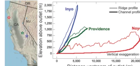
in-Figure 1.Study site locations and comparison of channel and ridge profiles. Left: location map of study catchments in California, USA. Right: elevation longitudinal profiles of the lowest point at each travel distance (i.e., the main-stem channel) and the highest point at each travel distance (referred to here as the ridge profile). The longest and shortest travel distances in each catchment are the points where the two profiles meet. The channel and ridge profiles enclose all paired values of elevation and travel distance for each catchment. Differences in catchment relief and size across the sites produce distinct populations of paired values. The ratio of elevation to travel distance is the mean slope along a path from the source to the catch-ment outlet. Thus, the catchcatch-ments also harbor distinct populations of mean slope.
fluenced by hillslope sources of water, solutes, and sediment (e.g., Lukens et al., 2016).
2 Elevation and travel distance in natural landscapes
Table 1.Study site characteristics.
Inyo Creek Providence Creek Noyo River
Drainage area (km2) 3.4 8.1 144
Relief (m) 1895 1117 893
Max travel distance (m) 4660 7940 20 790
Mean slope to outlet 0.33 0.14 0.021
Elevation of outlet (m a.s.l.) 2053 998 84 Outlet UTM north (m) 392 369.717 300 456.028 364 182.531 Outlet UTM east (m) 4 049 943.32 4 101 509.08 450 994.25
2.1 Study sites
The Inyo Creek catchment spans 2 km of relief over 4 km of travel distance on the eastern slope of the High Sierra (Ta-ble 1). Unlike some of its neighboring catchments along the range, it has never been scoured by glaciers, making it ideal for comparison of sediment production and landscape evo-lution in glaciated and non-glaciated terrain (Riebe et al., 2015; Stock et al., 2006; Brocklehurst and Whipple, 2002). Moreover, the catchment spans a range in the relative impor-tance of physical, chemical, and biological weathering from its warm, gently sloped, low elevations to its cold, steep head-waters.
On the other side of the Sierra Nevada, Providence Creek spans 1 km of relief over 8 km of travel distance (Table 1). This catchment is part of the Southern Sierra Critical Zone Observatory, which has been the focus of numerous recent studies of hydrology, biogeochemistry, and geomorphology (e.g., Bales et al., 2011; Hunsaker and Neary, 2012; Hun-saker et al., 2012; Goulden and Bales, 2014; Holbrook et al., 2014; Hahm et al., 2014). Precipitation in the upper half of the catchment dominantly falls as snow, whereas precipita-tion in the lower half dominantly falls as rain. Unlike the roughly continuous concave ridge and channel profiles of Inyo Creek, catchment topography in Providence Creek ex-hibits a pronounced step in elevation of both the channel and ridge profiles (Fig. 1). Steps like these, which are common on the southwestern slope of the Sierra Nevada, have been inter-preted to reflect a feedback between weathering and erosion (Wahrhaftig, 1965).
Farther to the northwest, in the California Coast Ranges, the Noyo River catchment spans 0.9 km of relief over 20 km of travel distance. Thus, the catchment is significantly larger and more gently sloped on average than either of the other two study catchments. The catchment has a long history of intensive timber harvests and has been the site of numerous studies of the effects of land use on in-stream habitat (Burns, 1972; Lisle, 1982; Leithold et al., 2006) and the role of to-pography and channel network structure in the production and delivery of sediment from slopes to channels (Dai et al., 2004; Sklar et al., 2006).
2.2 Spatial distributions of elevation and travel distance The maps in Fig. 2 show the spatial distributions of ele-vation and travel distance across each catchment. Broadly, travel distance and elevation covary in space; the highest el-evations in each catchment tend to be further away from the outlet. However, in detail, elevation contours are not aligned with contours of equal travel distance; the elevation contours exhibit higher planform curvature than travel distance con-tours. This pattern is especially clear at Inyo Creek (Fig. 2a) and Providence Creek (Fig. 2b), which drain small, rela-tively undissected catchments. In particular, as can be seen in Fig. 2a by following a given elevation contour (black lines), travel distances (color bands) are longest in the valley axis and shortest at the ridges. Conversely, for a given travel dis-tance (i.e., following a boundary between color bands), ele-vations are highest at the ridges and lowest in the valley axis. The patterns in elevation and travel distance in the Noyo River catchment are more complex (Fig. 2c), in part be-cause it is more deeply incised by multiple high-order trunk streams. At ridges that separate these trunk streams, travel distance can vary considerably from one side of the ridge to the other. Thus, nearby points that share the same eleva-tion can have very different travel distances. For example, along the central ridge, which runs along the catchment’s axis, points on the south side of the ridge drain to a more sinuous and thus longer southern trunk stream, giving them longer travel distances to the outlet than points on the north-ern side. For the same travel distance, points occur at higher elevations in the sub-catchment of the northern, less sinuous trunk stream.
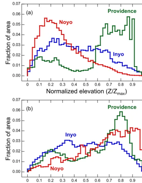
2.3 Hypsometry and the width function
(a)
(b)
(c)
Figure 2. Spatial distributions of elevation and travel distance. Maps showing the spatial distribution of elevation and travel dis-tance across the Inyo Creek(a), Providence Creek(b), and Noyo River(c)study catchments. Black lines are elevation contours, with hillshade in background for emphasis. Color shade shows scaled values of travel distance (normalized by the maximum value in the catchment). Note variation in scale and compass orientation from one watershed to the next. Elevation contour spacing is 50 m in(c)
and(b)and 200 m in(c).
occurs at higher elevations, above the pronounced step in the topography. Meanwhile, at the Noyo River site, the majority of area occurs at lower elevations, because the catchment is deeply dissected, with wide valley bottoms and steep, narrow ridges.
Hypsometry reveals differences in the vertical structure of the catchments, whereas the width function reveals differ-ences in planform structure, which are governed in part by differences in the shapes of the catchment boundaries. For
0.00 0.01 0.02 0.03 0.04 0.05 0.06 0.07
0 0.1 0.2 0.3 0.4 0.5 0.6 0.7 0.8 0.9 1
Fraction of area
Normalized elevation (Z/Zmax)
Inyo
Providence
Noyo
(a)
0.00 0.01 0.02 0.03 0.04 0.05 0.06 0.07
0 0.1 0.2 0.3 0.4 0.5 0.6 0.7 0.8 0.9 1
Fraction of area
Normalized travel distance (X/Xmax)
Inyo
Providence
Noyo
(b)
Figure 3.Hypsometry and width functions. Normalized frequency distributions of elevation(a)and travel distance to the outlet(b). Frequencies are normalized so that the area under the curve is equal to 1 in each case. Binning increment is 1/47 of maximum value (Table 1).
example, the distribution of travel distances at Inyo Creek is symmetrical, reflecting the roughly oval shape of the catch-ment. Meanwhile, at Providence Creek, the distribution of travel distances is bimodal, reflecting the narrowing near the middle of the catchment. At the Noyo River site, the travel distance distribution is skewed, with the majority of the area at long travel distances, reflecting the widening of the catch-ment with increasing distance from the outlet that is evident in Fig. 2c.
(a)
(b)
(c)
(d)
(e)
(f)
Elevation above outlet (m)
Elevation above outlet (m)
Elevation above outlet (m) Elevation above outlet (m)
Elevation above outlet (m)
Elevation above outlet (m)
Distance upstream of outlet (m) Distance upstream of outlet (m)
Distance upstream of outlet (m) Distance upstream of outlet (m)
Distance upstream of outlet (m) Distance upstream of outlet (m) Normalized density
Vertical exaggeration = 4
Vertical exaggeration = 12
Vertical exaggeration = 1.2
Figure 4.Joint distributions of elevation and travel distance. Distribution of source-area elevations and travel distances from 10 m DEMs of catchments drained by(a)Inyo Creek,(b)Providence Creek, and(c)the Noyo River. Bivariate frequency distributions of elevation and travel distance for each catchment(d–f)show relative density (color bar ind); data binning as in Fig. 2.
These differences likely correspond to differences in factors such as water-transit times, sediment breakdown rates, and channel morphology. Although information on the distribu-tion of mean slopes is embedded in both the hypsometry and the width function, it cannot be extracted from either of them plotted alone or even plotted side by side (Fig. 3).
To overcome the limitations of separate plots of verti-cal and horizontal structure, we plotted the joint distribution of elevation and travel distance for every point in each of the catchments in Fig. 4. These plots show both the longi-tudinal profile of the channel network and the distribution of hillslope sources, which account for more than 98 % of the source area in each catchment. A number of similarities emerge across the sites (Fig. 4a–c). Strikingly, at the highest elevations for any given travel distance, sources are aligned in steeply sloped tendrils of data that coalesce at lower el-evations. These tendrils represent hillslope sources aligned along common flow paths that cluster together into narrow groups. Equally striking are the gaps between the tendrils, which represent paired values of elevation and travel distance that do not occur anywhere in the catchment. Meanwhile, many paired values are so common that they overlap,
par-ticularly along flow paths that converge near the main-stem channel.
Bivariate frequency distributions help shed light on the degree of clustering and overlap of data at shared values (Fig. 4d–f). These binned representations of the raw data show that, for a given travel distance, the lowest point densi-ties (point area=100 m2) generally occur at the highest rel-ative elevations. As relrel-ative elevation decreases within a ver-tical stack of data, point density typically increases to a peak and then approaches zero at the channel elevation. In general, peak densities for a given travel distance occur closer to the channel than the ridge elevation, although there are notable exceptions. Figure 4d–f also show that the greatest frequency of the high point density (normalized density > 0.6) primarily occurs in the upper third of Inyo and Providence Creeks, and in the upper half of Noyo River.
Inyo Creek
Providence
Creek
Noyo
River
(a)
(b)
(c)
(d)
(e)
(f)
Mean slope on travel pathElevation above outlet (m)
Distance upstream of outlet (m)
Elevation above outlet (m)
Distance upstream of outlet (m)
Elevation above outlet (m)
Distance upstream of outlet (m)
Mean slope on travel path
Mean slope on travel path
Figure 5.Distribution of mean slope across catchments. Histograms (insets,a–c) of mean slope along travel path from source to outlet (ratio of source-area elevation to travel distance), with colors highlighting bins of relatively low, medium, and high values. Bins of common mean slope form linear bands on plots of elevation vs. travel distance (a–c). Maps of catchments (d–f) show spatial distribution of source areas sharing similar mean slope for highlighted values.
mean that the highest densities of catchment area occur at points that have both long travel distance and low elevation. Rather, low elevations dominate across all travel distances, and summing area horizontally across Fig. 4f leads to higher total area in the lower elevation bins of Fig. 3a. Similarly, the Noyo catchment has greater relief at longer travel distances, and summing area vertically across Fig. 4f leads to higher total area in the longer travel distance bins of Fig. 3b. This comparison demonstrates that the joint distribution of eleva-tion and travel distance reveals where area is distributed in the vertical and horizontal structure of the catchment in ways that the hypsometry and width function cannot.
Comparisons of the joint distributions between catchments also reveal significant differences that cannot be inferred from the conventional representations of vertical and hori-zontal catchment structure in Fig. 3. For example, the rela-tive slopes of the tendrils and the channels differ markedly. The tendrils are much steeper than the main-stem channel profile in the Noyo River catchment (Fig. 4f). Conversely, in
the other two catchments, the tendrils and the main channel profile have similar slopes, especially at Providence Creek. These differences likely arise at least in part due to the differ-ence in scale of the watersheds; in the Noyo River catchment, some of the individual tendrils encompass large areas, similar in scale to the entire Inyo and Providence Creek catchments. Thus, we interpret the tendrils along the Noyo River to be tributary catchments that are similar to the Inyo and Provi-dence Creek catchments, with tendrils of their own that are only slightly steeper than the local tributary channel slopes.
elevation and travel distance (Fig. 2). Mean slopes are rela-tively steep and span a relarela-tively narrow range at Inyo Creek (Fig. 5c) compared to the Noyo River catchment (Fig. 5f). Providence Creek is distinguished by a peak in mean slopes (Fig. 5b) corresponding to the upper half of catchment, above the step in the topography (Fig. 5e).
Mean slope quantifies the ratio between elevation and travel distance and thus is a single metric that combines two fundamental attributes of source areas in catchments. The distributions of source elevation, travel distance, and thus mean slope are ultimately set by the erosion and transport processes that produce and deliver sediment from slopes to channels. Thus, spatial variations in mean slope, such as those shown in Fig. 5, may be closely linked to spatial vari-ations in the production and delivery of water, solutes, and sediment.
3 Source-area and catchment power
To develop a mechanistic framework for linking distributions of source-area mean slope with catchment processes, we in-troduce the concept of source-area power, which combines elevation, travel distance, and the production rate of mate-rial on slopes. In the derivation that follows, we consider a massMof transportable material (such as water, solutes, or sediment) produced at a source elevationzand transported downstream by a distanceLto an elevationzoat the
catch-ment outlet. The potential energy (E) of the material at the source, relative to the outlet is given by Eq. (1):
Ei,j =Mi,jgRi =ρi,jAihi,jg(zi−zo). (1)
Here g is acceleration due to gravity, R is relief (i.e., the difference in elevation between the source and outlet), ρ is density, h is the thickness of the material produced at the source, A is the area of the source (one pixel in a DEM), the subscriptirefers to the specific source location, and the subscriptj refers to the type of material (e.g., water, solutes, or sediment). In the case of solutes,hrefers to the equivalent thickness of chemical erosion needed to account for the mass loss due to production of solutes.
At each source, potential energy is produced at a rate () that is proportional to the production rate (Q) or flux of ma-terial from the source, as shown in Eq. (2):
i,j =Qi,jgRi =ρi,jAi
∂hi,j
∂t g(zi−zo). (2)
Here, the definition of ∂h/∂t (in dimensions of length per time) depends on the process considered. For water produced by precipitation,∂h/∂tis the precipitation rate. For sediment produced by erosion,∂h/∂tis the physical erosion rate. For solutes produced by chemical erosion,∂h/∂t is the equiva-lent to the chemical erosion rate. In all cases,has dimen-sions of power.
On its journey to the outlet, the material loses its poten-tial energy. This energy is converted to kinetic energy and is
primarily lost to heat due to friction. In the case of sediment, some of the energy is consumed when particles are abraded and shattered during collisions with other particles and the channel bed. Thus, it may be useful in the context of geo-morphic work to think of the power expended by the water or sediment over the travel distance (L) between the source and outlet, as shown in Eq. (3):
ωi,j =
Qi,jgRi
Li
=ρi,jAi
∂hi,j
∂t g
(zi−zo)
Li
. (3)
We refer to ω as “source-area power”, which has dimen-sions of power per length, where (zi-zo)/Liis the mean slope
along the travel path from the source to outlet.
Source-area power is distinct from stream power, which is how energy dissipation in landscapes is commonly quan-tified (Rodríguez-Itrube et al., 1992; Lague, 2014). Stream power uses the entire upstream contributing area to calculate the material flux, whereas the contributing area for source-area power is limited to the smallest unit of analysis, such as a single pixel in a DEM. Moreover, stream power quantifies the local rate of energy dissipation across a short distance, such as a reach of river represented by the distance between two pixels, whereas source-area power averages energy dis-sipation over the entire travel distance from source to catch-ment outlet. Hence, unlike stream power, source-area power quantifies the production rate of material potential energy in terms of the vertical and horizontal position of the source location relative to the catchment outlet. This provides a dis-tinct metric for analyzing spatial patterns in how energy is produced and dissipated within catchments.
The concept of source-area power allows us to explore the possible implications of variability in the ratio of elevation to travel distance (i.e., the mean slope) on the production and delivery of water, solutes, and sediment across catchments. For example, in landscapes where the rate of precipitation or erosion is spatially uniform, we expect the distribution of source-area power for the water or sediment to be identical to the distribution of the mean slopes of source areas. In con-trast, in landscapes where rates of precipitation and erosion are spatially variable and sometimes correlated (Reiners et al., 2003; Burbank et al., 2003), we expect the distributions of power and mean slopes to differ. This is the case at Inyo Creek, where mean annual precipitation increases with ele-vation from 290 mm yr−1at the outlet to 710 mm yr−1at the catchment divide (Prism Climate Group, 2014), and the rate of production of sediment by erosion has been estimated to increase exponentially with elevation from 0.03 mm yr−1at
the outlet to 1.5 mm yr−1at the divide (Riebe et al., 2015).
(a) Precip. source-area power
(b) Erosion source-area power
(c) Precip. power per sed. flux
Source-area power (W m x 10 )-1 -3Source-area power (W m x 10 )-1 -3
Figure 6.Spatial distribution of source-area power for water and sediment. Histograms (left) of source-area power calculated using Eq. (3) for the Inyo Creek catchment for water delivered by precipitation(a)and sediment produced by erosion(b). Panel(c)shows dimensionless ratio of source-area water power to sediment production rate (Eq. 4); colors highlight bins of relatively low, medium, and high values. Maps (right) show spatial distribution of highlighted values. Note the sharp increase in water power per sediment flux from upper to lower parts of the catchment.
divide, relative to the case of uniform precipitation and ero-sion (equivalent to Fig. 5a). The difference is greatest for the case of spatially varying erosion (Fig. 6b), due to the nonlin-ear relationship between erosion rate and elevation. Thus, for catchments with spatial variation in the rate of production of water or sediment, mean slope distributions cannot reliably predict distributions of source-area power.
Comparisons of source-area power and production rates for different materials may provide insight into the spatial variation of catchment processes. For example, sediment pro-duced by erosion at source areas is transported to the out-let by a combination of primarily gravity-driven processes, including creep and landslides, and by water-mediated pro-cesses such as overland, debris, and fluvial flows. Catchment topography, as expressed in the joint distribution of elevation and travel distance, may reflect the spatial variation and rela-tive importance of these different processes. Because the al-titudinal gradients in erosion and precipitation at Inyo Creek are known, we can use them to explore how the source-area power of water, relative to the amount of sediment that must be produced on hillslopes and transported to the outlet, varies across the catchment assuming steady state. We define
a dimensionless ratio (ω∗i,w/s) that quantifies the source-area power of water per mass of sediment eroded at an individual pixel,i:
ωi,∗w/s= ωi,w
gQi,s
=ρw ∂hi,w/∂t
ρs ∂hi,s/∂t
(zi−zo)
Li
. (4)
(e.g., via sheetwash and channelized flow), and that weath-ering is dominated by chemical processes. This is broadly consistent with field observations: headwater slopes consist of steep, landslide-dominated bare bedrock, whereas slopes near the catchment outlet are gentler, more vegetated, and soil mantled, implying that chemical weathering is favored by longer residence times of water and sediment (Riebe et al., 2015).
Power for a given material can also be characterized at the scale of whole catchments. To do this, we sum Eq. (3) over the entire contributing area, using Eq. (5):
ωc,j =g
i=N X
i=1
ρi,jAi
∂hi,j
∂t
(zi−zo)
Li
. (5)
Here ωc,j is the catchment-integrated source-area power
for the material of interest j, or, more simply, “catchment power”. It expresses the total power expended as the poten-tial energy of material produced throughout the catchment is lost along flow paths to the outlet. For Inyo Creek, the to-tal catchment power for water is 166 W m−1, while the total catchment power for sediment is 0.122 W m−1. The ratio of catchment power for water to sediment is 136. This ratio re-flects the combined effects of the steep altitudinal increase in erosion rates, the more modest altitudinal increase in precip-itation rates, and how these trends map onto the joint distri-bution of elevation and travel distance.
New theory and data from other landscapes are needed to interpret spatial variations in power across individual catch-ments and to understand why they vary from catchment to catchment. For example, we might expect to find a differ-ent spatial distribution of water-sedimdiffer-ent power ratios, rela-tive to Inyo Creek, in a catchment with a different hypsom-etry and width function. Likewise, the spatial distribution of source-area power would differ greatly in a catchment re-sponding to accelerated base-level lowering, with faster ero-sion rates near the outlet. More generally, we might expect the ratio of water to sediment catchment power to vary con-siderably from catchment to catchment across gradients in climate and tectonics. Understanding these variations could provide fresh insights into the geomorphic processes that shape landscapes.
Although our analysis of power at Inyo Creek focused on the production of water and sediment, it can be extended to any material that varies in production rate with altitude or varies in delivery to the outlet as a function of travel distance. For example, production rates of solutes, nutrients, contam-inants, and even cosmogenic nuclides could be substituted for the production rate terms in Eqs. (2–5). Thus, it should be possible to use the new frameworks of source-area and catchment power to model, and therefore better understand, both the spatial distribution and catchment-integrated effects of geomorphic, geochemical, and ecosystem processes.
Our analysis of Inyo Creek shows how the power frame-work can be applied to natural landscapes using a DEM.
However, factors, such as climate, topography, and tecton-ics, which might influence power and thus merit further in-vestigation, are closely coupled together. This makes it diffi-cult to isolate any single factor of interest in comparisons of power across catchments. Moreover, some catchments, such as Providence Creek, have peculiarities in shape and struc-ture that dominate patterns of power (Fig. 5b) and thus might confound comparisons of one catchment to the next. To over-come the limitations of using DEMs from individual catch-ments, we developed an approach that generates synthetic catchments based on scaling relationships for catchment ge-ometry and topography. With this approach we can system-atically explore how variations in factors such as area, relief, and profile concavity influence the distribution of source-area and catchment power in landscapes. In the next section we show that our synthetic catchments capture the fundamental characteristics of the joint distribution of elevation and travel distance in landscapes and thus can be used to isolate and study the influence of the physical, chemical, and biological factors that govern catchment processes.
4 Synthetic joint distributions of elevation and travel distance
Our objective in developing synthetic catchments is to gener-ate realistic joint distributions of elevation and travel distance (e.g., that are comparable to those shown in Fig. 3). Equa-tions (3–5) show that this should be sufficient to quantify dis-tributions of source-area and catchment power. Hence, there is no need for a spatially explicit representation of topogra-phy, because calculating source-area power does not require information about spatial position of channels or topographic factors such as hillslope gradient or curvature. Populating the joint distribution of elevation and travel distance only re-quires specifying the upper and lower elevation boundaries at each travel distance and then distributing area across eleva-tions in the space between the boundaries. Although theory is available to generate main-stem longitudinal profiles that could serve as a realistic lower boundary of the distribution, we are unaware of any theory for predicting ridge profiles and thus delineating a realistic upper boundary. Most im-portantly, to our knowledge, no theory is available for pop-ulating the elevation distribution for a given travel distance between the upper and lower boundaries, without creating a spatially explicit synthetic DEM using a landscape evolution model (Coulthard, 2001; Willgoose, 2005; Tucker and Han-cock, 2010).
0 500 1,000 1,500 2,000
0 1,000 2,000 3,000 4,000
Elevation above outlet (m)
Distance upstream of outlet (m) Inyo Creek
(a)
0 400 800 1,200 1,600
0 500 1,000 1,500 2,000
Area (m
2)
Elevation above outlet (m)
(b)
L = 550 2250 1350 3050
3650
4050
4350
0 0.01 0.02 0.03 0.04
0 0.01 0.02 0.03 0.04
Fraction of total area in bin
Fraction of total relief in distance bin
(c) 1:1 line
0 0.01 0.02 0.03 0.04 0.05 0.06 0.07
0 0.2 0.4 0.6 0.8 1
(Elevation - min elevation) / relief
Fraction of area
(d)
Best-fit beta distribution
Figure 7.Elevation distributions for different travel distances at Inyo Creek.(a)Elevation data points for Inyo Creek catchment parsed into forty-seven 100 m wide travel distance bins.(b)Distributions of elevation for seven representative travel distance bins; colors correspond to shaded bins in panel(a), and mean travel distance is indicated for each curve.(c)Fraction of total area in each travel distance bin as a function of fraction of total relief in each bin, roughly follows the 1:1 line, colored symbols indicate representative bins in panels(a)and
(b).(d)Collapse of elevation distributions for each travel distance bin, with elevation normalized by relief within bin and area by total area within bin. Best-fit beta distribution captures typical shape of hypsometry for a given travel distance.
boundaries at each travel distance and use the best-fit area-vs.-elevation function to define a fully synthetic joint distri-bution of elevation and travel distance.
4.1 Area-vs.-elevation at each travel distance
To find the best-fit relationship between area and elevation at each travel distance, we parsed the Inyo Creek catchment into forty-seven 100 m wide travel distance bins (Fig. 7a). Figure 7b shows distributions of area with elevation for seven representative travel distance bins. Inspection of Fig. 7b sug-gests that the area under the curves scales with local relief (i.e., the width across the base of the curve), and that the distributions are consistently right skewed, with more area at the lower elevations. When we sum area and relief across all bins, and plot the fractional area vs. fractional relief for each bin, we find that the data roughly follow a 1:1 line (Fig. 7c). We obtain a similar result for a variety of bin spac-ings, which suggests that the area–elevation relationship is self similar: when the upper and lower boundaries are far-ther apart (i.e., when local relief is higher), the area contained within the travel distance bin increases in direct proportion to the difference in relief. This permits a collapse of the distri-butions of elevation for each travel distance bin, by normal-izing elevation with local relief and area by total area in the bin. Figure 7d shows the normalized hypsometry for travel distance bins spanning the entire Inyo Creek catchment. The broad consistency of the shapes of the normalized
distribu-tions suggests that a single functional form could represent the central tendency, spread, and even the skew of the distri-bution of area with elevation for any travel distance across the catchment.
The beta distribution has a simple functional form that captures two key characteristics of the normalized area– elevation relationships: it is bounded by 0 and 1, and it can have right skew depending on the values of its two shape factors,αandβ. Thus, a beta distribution is well suited to generating synthetic distributions of area as a function of el-evation.
A generic form of the beta distribution is shown in Eq. (6):
fβ=xα−1(1−x)β−1. (6)
Herefβis the height of the beta distribution at pointx, where
xranges from 0 to 1 and the sum of area under the curve is equal to 1.
To find the values ofαandβ that correspond to the best fit between the area–elevation data and the beta distribution across all travel distances at Inyo Creek, we first converted Eqs. (6) to (7) for dimensional consistency.
fA(z, L)=AL z∗
α−1
1−z∗β−1
(7)
Here,fA(z, L) is the height of the scaled beta distribution
at elevationzin travel distance binL,AL is the area in the
travel distance bin, andz∗=(z−zC)/(zR−zC), wherezC
is the elevation of the channel andzRis the elevation of the
Alpha (shape factor 1)
Beta (shape factor 2)
Figure 8.Objective function for best-fit beta distribution shape pa-rameters. Contour plot of root mean sum of squared error (RMSE) between actual and predicted area density of elevation for a given travel distance for paired values of beta distribution shape param-eters. Minimum RMSE atα=2.6 andβ=3.4 as indicated by the diamond. In this example, travel distance and elevation bin sizes equal 100 and 40 m, respectively.
By applying Eq. (7) to each travel distance bin, we can generate a synthetic joint distribution of elevation and travel distance. We then can calculate the misfit between the syn-thetic and actual joint distributions as the square root of the mean squared differences (RMSE) at each elevation and travel distance. To find the best-fit parameters, we used an optimization algorithm to search for the pair of shape factors that minimize the misfit. For Inyo Creek data, with 100 m travel distance bins, and 40 m elevation bins (Fig. 7), the best-fitαis 2.6 and best-fitβis 3.4. The objective function for this case is shown in Fig. 8. The best-fit parameters yield a beta distribution that follows the trend in the normalized area dis-tributions shown in Fig. 7d.
To quantify the model performance, we use the Nash– Sutcliffe model efficiency statistic (NS) (Nash and Sutcliffe, 1970), which is calculated as
NS=1−
P
(fA-Model−fA-Data)2
P(f
A-Mean−fA-Data)2
. (8)
Here the subscript “Model” refers to the predictions of Eq. (7), “Data” refers to the DEM, and “Mean” represents a uniform area density in each bin equal to the total area divided by the number of distance and elevation bins con-taining data. A model efficiency of 1 implies a perfect match between predictions and observations. An efficiency of 0 in-dicates that model predictions are only as accurate as sim-ply using the mean of the observed data. Less than zero ef-ficiency (NS < 0) implies that the observed mean is a better predictor than the model. In other words, the closer the model
0.0 0.1 0.2 0.3 0.4 0.5 0.6 0.7 0.8 0.9 1.0
100 1,000
Nash–Sutcliffe statistic
Travel distance bin size (m)
100
Z_bin (m)
70
10 40
Profiles Actual Model
Figure 9.Model performance. Variation in Nash–Sutcliffe model efficiency statistic (Eq. 8) with size of travel distance and elevation bins, for modeled joint distributions of elevation and travel distance for Inyo Creek, using actual profiles (solid lines) and modeled pro-files (dashed lines). A Nash–Sutcliffe value of 1.0 indicates per-fect agreement between modeled and actual distribution of area; a value of 0 indicates model performance no better than uniform dis-tribution of mean area density. A tradeoff between model efficiency and spatial resolution is revealed by the trend toward higher Nash– Sutcliffe values for larger bin sizes.
efficiency is to 1, the more accurate the model is. For this par-ticular binning scheme (100 m distance and 40 m elevation bins), the Nash–Sutcliffe model efficiency statistic for Inyo Creek is 0.41, indicating good but not excellent agreement with the topographic data.
To explore the sensitivity of model performance to spatial resolution of the binning scheme, we repeated the optimiza-tion procedure described above for a range of travel distance and elevation bin sizes. As shown in Fig. 9a, the NS val-ues are generally higher for larger bin sizes (i.e., fewer bins), reaching a local maximum (NS > 0.7) for 400 m travel dis-tance bins. Model efficiency approaches 1.0 (NS > 0.9) for a single distance bin, which is equivalent to fitting the whole catchment hypsometry with a single beta distribution curve.
These results reveal a tradeoff between model perfor-mance and spatial resolution. They also suggest that, to first order, Eq. (7) can capture much of the structure of area as a function of relief at Inyo Creek. To the extent that we can think of Inyo Creek as a prototypical catchment, we can use Eq. (7) to generate synthetic joint distributions of elevation and travel distance for other catchments, with different chan-nel and ridge profiles.
across elevations but also produces synthetic channel and ridge profiles that define the upper and lower boundaries of elevation as a function of travel distance.
4.2 Main-stem channel and ridge profiles
For any travel distance, the lowest elevation will be on the channel main stem. Thus, the main-stem longitudinal profile is the lower boundary for the joint distribution of elevation and travel distance. Channel elevations (zC) are commonly
modeled as a power function of travel distance (x) along the main stem from the outlet to the upstream limit of fluvial pro-cesses (i.e., the distance to the “channel head”, denotedxch).
As elaborated in the Appendix, here we derive an expression for channel elevation that extends all the way to the top of the catchment, at the point where the valley axis meets the drainage divide.
From the outlet toxch, the elevation of the channel can be
written as
zC=kC
h
(Lmax)1−θ H−(Lmax−x)1−θ H i
for 0≤x≤xch. (9a)
Here,Lmax is the travel distance to the outlet from the
fur-thest point in the catchment, θ andH are the exponents in Flint’s law and Hack’s law, respectively, andkCis a constant
that lumps togetherθ,H, and other factors, as shown in the Appendix A.
For the valley axis upstream of the channel head, fromxch
toLmax, the elevation profile can be written as follows (see
Appendix A for derivation):
zC=kC
h
(Lmax)1−θ H−(Lch)1−θ H i
+Sh(x−xch)
forxch< x≤Lmax. (9b)
Here,Lchis the distance from the channel head to the outlet
andShrepresents a uniform slope over the distance between
LchandLmax.
The upper boundary of the joint distribution of elevation and travel distance is defined by the collection of points at the highest elevations in each travel distance bin. Unlike the channel profile, which defines the base of the joint distribu-tion, the points at the upper boundary do not necessarily lie along a contiguous path. Nevertheless, for simplicity we refer to these points as the ridge profile and assume that its eleva-tion follows a simple power-law relaeleva-tionship with distance:
zR=kRxP. (10)
HerekR is an adjustable parameter and the exponentP
de-pends on the parameters of the channel profile. As elaborated in the Appendix, we impose the constraints that the ridge pro-file intersects the main-stem channel propro-file at the two end points, wherex=0 andx=Lmax, in order to define the
pa-rameterP.
4.3 Scaling between area and relief
Equations (9) and (10) provide the values ofzCandzRthat
are needed in Eq. (7) to define the local relief for any travel distance. However, before Eq. (7) can be used to generate synthetic distributions of elevation and travel distance, the area in each travel distance bin (AL) must be defined. We
do so using the previously discussed self-similar relationship between area and local relief shown in Fig. 7c, where the fraction of the total area in a travel bin of interest is propor-tional to the local relief divided by the sum of local relief over all travel distance bins. For Inyo Creek, this relation-ship holds for any choice of bin spacing and it is expressed mathematically in Eq. (11):
AL
AC
= AL
N P
L=1
AL
= RL
N P
L=1
RL
. (11)
Here,N is the number of bins; AC is the catchment area,
which is equal to the sum of all AL; and RL is the relief
in the travel distance bin, which is equal tozR-zC.
Follow-ing Hack’s law, the total area of the catchment (AC) can be
treated as a power function ofLmax(see Appendix A).
4.4 Generating synthetic distributions of elevation and travel distance
1 2 3 4 5 6 7 x 10⁻³
Width Func+on
Hyposom
etr
ic
Cur
ve
Synthe+c Catchment
(a) (b)
(c)
Area fraction
Area fraction
Width function
Synthetic catchment
Distance upstream of outlet (m)
Elevation above outlet (m)
Hypsometric curve
Figure 10.Fully synthetic joint distribution of elevation and travel distance for catchment the size of Inyo Creek. In(a), channel and ridge profiles are defined by Eqs. (9) and (10), and area density (color bar) is given by Eqs. (7) and (11). Side panels show area density projected on distance axis to create width function(b)and projected on elevation axis to create hypsometric curve(c).
0 0.05 0.1 0.15
Fraction of area
Providence Creek
α = 1.9; β = 2.3 (a)
0 0.05 0.1 0.15
0 0.2 0.4 0.6 0.8 1
(Elevation - min elevation) / relief
Fraction of area
Noyo River α = 1.7; β = 2.8
(b)
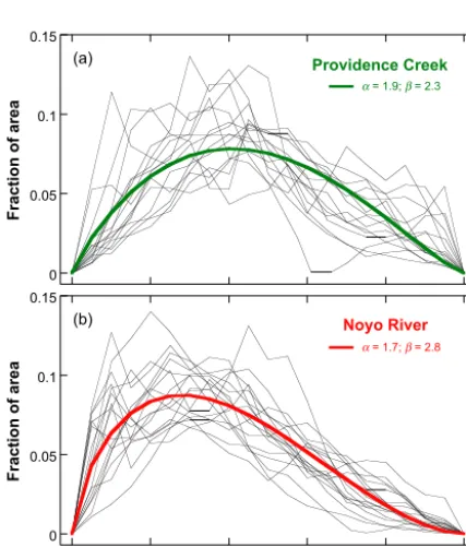
Figure 11. Normalized distribution of elevation by travel dis-tance bin for other catchments. Travel disdis-tance and elevation bin sizes=1/20 of maximum values. Thin lines show elevation dis-tributions, normalized by local relief, for each travel distance bin. Thick colored curves show best-fit beta distributions, with shape parameter values indicated. Normalized elevation distributions are more skewed for Noyo River, reflecting larger drainage area and greater degree of landscape dissection.
5 Discussion
5.1 Extending the model to other catchments
The fully synthetic formulation for the joint distribution of elevation and travel distance was calibrated using data from Inyo Creek, under the assumption that it is a proto-typical catchment. However, Inyo Creek is relatively small and steep. This raises the question of whether the synthetic formulation yields realistic results in other landscapes with lower relief or higher area.
0.00 0.01 0.02 0.03 0.04
Fraction of area
DEM
4.2 5.7
Hypsometry
0.00 0.02 0.04 0.06
0 0.1 0.2 0.3 0.4 0.5 0.6 0.7 0.8 0.9 1
Fraction of area
Normalized elevation (Z/Zmax)
DEM
2.1 9.2
0 0.1 0.2 0.3 0.4 0.5 0.6 0.7 0.8 0.9 1 Normalized travel distance (X/Xmax)
DEM
7.8
Noyo River
10.1
DEM
12.3
Providence Creek
14.2
0.00 0.02 0.04 0.06
Fraction of area
DEM
12.5 15.7
Synthetic joint distributions
with modeled profiles with actual profiles
4.6 Inyo Creek
5.0
Width function
DEM
Figure 12.Comparison of actual with modeled hypsometric curves and width functions for three study catchments. In each panel, thick colored curves show data from catchment DEM, while thick and dashed black lines show model predictions using actual and modeled channel and ridge profiles, respectively. Values in parentheses indicate RMSE calculated by comparing model curves with DEM.
The three catchments we analyzed vary not only across gradients in relief and drainage area (Fig. 1) but also in the degree of dissection and channel profile shape, which may in turn reflect differing lithologic, tectonic, or climatic bound-ary conditions. For example, Providence Creek has a pro-nounced step in the channel profile, with greater local re-lief and area concentrated in the upper part of the catchment (Fig. 2). This step may arise due to feedbacks between weath-ering of biotite and topographic slope across the landscape (Wahrhaftig, 1965). As a result, the channel profile is not well fit by a power equation or any other simple function. In contrast, the larger Noyo River catchment has a smooth, highly concave main-stem channel profile, and greater area at longer travel distances to the outlet due to a high degree of channel branching. The Noyo River main-stem channel pro-file may be influenced by aggradation due to sea-level rise, and is better represented in the fully synthetic model using an exponential equation instead of a power equation (see Ap-pendix A).
Another second way to gauge model performance for var-ious catchments is to compare predicted hypsometric curves and width functions using the projections of the modeled
here, provided that variations in the channel profile can be modeled.
5.2 Future research opportunities
Our results suggest many potentially fruitful avenues for fu-ture research. First, joint distributions of travel distance and elevation, combined with knowledge of rates of precipitation, erosion, or other material fluxes, can be used to understand how energy is created and dissipated across landscapes. The concept of source-area power provides a quantitative mea-sure of the spatial distribution of processes that influence the supply of materials to the catchment outlet. For example, this framework can be used to understand how the size distribu-tion of sediments passing through a catchment outlet is influ-enced by weathering conditions at source elevations (Sklar et al., 2016), and by particle breakdown in transport (Attal and Lavé, 2009). Specifically, the initial particle size produced on hillslopes may vary systematically with local climate, vege-tation, and erosion rate, factors that commonly vary with ele-vation within catchments (Riebe et al., 2015). In the absence of particle size reduction in transport, the size distribution of sediments delivered to the outlet would then reflect the distribution of source elevations, weighted by the local ero-sion rate. Yet particle wear is likely to be significant except in small catchments underlain by exceptionally durable rock. The overall extent of particle size reduction in transport will depend on the distribution of travel distances and the rates of energy dissipation along those transport paths. Thus, the evo-lution of sediment sizes in catchments, from source areas to the catchment outlet, and the resulting size distribution pass-ing through the outlet, depend on the factors that together determine source-area power.
Second, catchment power, the integral of source-area power for a given material over the entire catchment (Eq. 5), provides a metric for comparisons between catchments, and could be used to quantify, and help explain, the variation in topography across gradients in climate, tectonics and lithol-ogy. For example, Reiners et al. (2003), found a strong cor-relation between spatial variation in erosion rate and precipi-tation in the Cascade Mountains of Washington but no corre-sponding trend in conventional topographic indices such as local relief. Catchment power, calculated for water delivered by precipitation, for sediment produced by erosion, or as the ratio of water to sediment power, could provide a metric that captures how topography varies across gradients in precipi-tation and erosion. In this way, catchment power could help explain how topography mediates the linkage between cli-mate and tectonics. Catchment power could also be used to compare numerical simulations of landscape evolution with real landscapes (Willgoose, 1994; Willgoose et al., 2003) and contrast terrestrial catchments with catchments on Mars or Titan, where the topography reflects differing gravitational accelerations, fluids, and rock properties (Mest et al., 2010; Burr et al., 2012).
A third set of research questions emerges from our ap-proach to modeling synthetic joint distributions of elevation and transport distance. What explains the common tendency for positive skew in the distribution of area with elevation for a given travel distance? What do differences in the strength of this asymmetry from one catchment to another tell us about landscape-forming processes? Why are area and local relief within a travel distance bin linearly proportional, and does this relationship hold across a wider suite of catchments? Can the model of a fully synthetic catchment be used to represent landscapes across greater ranges of relief and drainage area than explored here?
Finally, the apparent success of our empirical model in capturing the bulk trends in the joint distribution of eleva-tion and travel distance in our study catchments suggests that there may be value in developing a more comprehensive model which accounts explicitly for the branching structure of the channel network. Such a model might have at its core a representation of the distribution of elevation and travel distance for a first-order catchment similar to our empirical model for Inyo Creek. The model would then represent larger catchments as combinations of multiple first-order headwa-ter sub-catchments, and the hillslope facets that drain directly to higher-order channel segments. This raises the question of whether there is a characteristic distribution of elevation for a given travel distance in the facets draining higher-order valley slopes, and whether it differs from the headwater sub-catchments in the same landscape. Variation in the topology of branching networks will shift the relative contributions of headwater sub-catchments and higher-order facets to the number of source areas at a given elevation or travel distance. How sensitive are the distributions of source-area power to variations in network topology? Ultimately, such a model may help explain both the central tendency and variability in the joint distribution of elevation and travel distance, and provide a stronger theoretical foundation for understanding the three-dimensional structure of catchment topography.
6 Summary
statistical framework for defining the joint distribution of ele-vation and travel distance. We used the Inyo Creek catchment as a prototype, and found that the distribution of elevation be-tween the main-stem channel and ridge profiles, for a given travel distance bin, is well represented by a parameterization of the beta distribution. To define a fully synthetic catchment, we derived power-law and exponential expressions for the channel and ridge profiles, which, when combined with the model for elevation distribution, can produce realistic hypso-metric curves and width functions. Key questions emerging from this work are as follows. How do patterns of source-area and catchment power vary across spatial
gradients in climate, tectonics, and lithology? What explains the characteristic skew of elevation distributions for a given travel distance? And how do the patterns in the distributions of source-area and catchment power arise from the branching properties of networks and the relief structure of landscapes?
7 Data availability
Appendix A: Derivation of channel and ridge profile equations
A1 Main-stem channel power-law profile
To create an expression for the longitudinal profile of the main-stem channel, we coupled the widely observed power-law scaling between slope (S) and drainage area (A),
S=ksA−θ, (A1)
and the likewise common power-law scaling of main-stem distance (L) and area,
A=kALH. (A2)
In Eq. (A1), known as Flint’s law, ks andθ are empirical
coefficients (whereθ is referred to as profile concavity). In Eq. (A2), a version of Hack’s law,Lis a local distance down-stream from the catchment divide along the main-stem val-ley axis, and kA andH are empirical coefficients (withH
the reciprocal of the Hack exponent). Hack’s law can also be written in terms of the local travel distance upstream of the catchment outlet,x,
A=kA(Lmax−x)H, (A3)
whereLmaxis the value ofLat the outlet (i.e.,x=Lmax−L).
Combining Eqs. (A1) and (A3) we obtain an expression for main-stem channel slope, Sc, as a function of distance
upstreamx,
Sc=
∂zc
∂x =ksk
−θ
A (Lmax −x)
−θ H, (A4)
wherezcis the elevation of the main-stem channel.
Integrating Eq. (A4) provides an expression for the main-stem longitudinal profile,
zC=kC
h
(Lmax)1−θ H−(Lmax−x)1−θ H i
, (A5a)
where
kC=
kskA−θ
1−θ H. (A5b)
Equation (A5) is valid for the fluvial portion of the chan-nel network. However, at small drainage areas, the fluvial slope-area scaling (Eq. A1) does not apply. Typically, slope changes much less rapidly as drainage changes in this part of the landscape. For simplicity we assume that slope is con-stant above a point on the longitudinal profile that we refer to as the channel head.
We define a distanceLchwhich is the travel distance from
where the valley axis meets the drainage divide down to the channel head; subscript ch indicates channel head. The el-evation at the channel head, wherex=xch=(Lmax −Lch)
is
zC=kC
h
(Lmax)1−θ H−(Lch)1−θ H i
. (A6)
The drainage area at the channel headAchis
Ach=kALHch, (A7)
and the constant gradient above this pointShis
Sh=ksA−chθ=
ks
kθAL
−θ H
ch . (A8)
Thus, the elevation of the longitudinal profile, from bottom to top, can be written as follows:
zC=kC
h
(Lmax)1−θ H−(Lmax −x)1−θ H i
for 0≤x≤xch, (A9)
zC=kC
h
(Lmax)1−θ H−(Lch)1−θ H i
+Sh(x−xch)
forxch< x≤Lmax. (A10)
The highest point along the main-stem profile,zC_max, is
zC_max =kC
h
(Lmax)1−θ H−(Lch)1−θ H i
+ShLch. (A11)
A2 Ridge power-law profile
To define the ridge longitudinal profile, we assume a simple power-law relation between elevation and distance,
zR=kRxP, (A12)
wherekRis an adjustable parameter and the exponentP
de-pends on the parameters of the channel profile. To specify P we impose the constraints that the ridge profile must in-tersect the main-stem channel profile at the two end points, wherex=0 andx=Lmax, the lowest and highest points in
the landscape.
With the constraints that the elevation of the ridgezRand
the channelzc match where x= 0 and x=Lmax, we can
solve for the exponentP as follows:
P =log zC_max/kR
log (Lmax)
. (A13)
Thus, the ridge network and the channel network are pinned together at the two end points.
A3 Inyo Creek power-law profile parameters
The combined model for the ridge and channel profiles has six parameters; all other values are calculated from the equa-tions above. For the Inyo Creek channel and ridge profiles extracted from the distributions of elevation for travel dis-tances binned in 50 m increments, Table A1 lists one pos-sible set of values that adequately reproduce the observed profile. These values were tuned to satisfy the following constraints:Lmax=4700 m, the range of travel distances of
Table A1.Inyo Creek power-law profile model parameters.
Parameter Value
θ 0.31
H 1.75
ks 25 m2θ
kA 1.28 m2−H
Lch 600 m
KR 0.6 m1−P
A4 Main-stem channel exponential profile
Exponential equations have been used in many previous anal-yses of river longitudinal profiles (e.g., Hack, 1973); eleva-tion of the channel is described as increasing exponentially with distance upstream of the outlet,
zc=keeλx, (A14)
wherekeandλare empirical coefficients. As with the power
profile, this is only valid in the fluvial portion of the profile, between the outlet and the channel head; above the chan-nel head, we assume the slope of the valley axis becomes uniform. For the exponential profile (Eq. A14), the channel slope,
Sc=
∂z
∂x =λkee
λx, (A15)
grows too slowly with increasing distance upstream of the channel head to represent the steep headwater valley axis slope, so we defineSh_expas an independent empirical model
constant, with the constraint that it must be greater than the slope of the exponential profile at the channel head,
Sh_exp > Sc_max =λkeeλ(Lmax−Lch). (A16)
The full channel profile expression becomes
zc=keeλxfor 0≤x≤xch, (A17a)
zc=keeλxch+S
h_exp(x−xch) forxch< x≤Lmax, (A17b)
and the highest point along the main-stem profile,zc_max, is
zc_max =keeλxch+Sh_expLch. (A18)
A5 Ridge exponential profile
To define the ridge longitudinal profile, for symmetry with the channel profile we assume an exponential relation be-tween elevation and distance,
zR=kReeγ x, (A19)
where the coefficientkReis an adjustable parameter, and the
exponentγdepends on the parameters of the channel profile.
Table A2.Noyo River exponential profile model parameters.
Parameter Value
λ 1.8×10⁻⁴m−1
Sh_exp 0.16
ke 6.7 m
Lch 2000 m
KRe 195 m
As with the power-law profile derivation, to specify γ we impose the constraints that the ridge profile must intersect the main-stem channel profile at the two end points, wherex=0 andx=Lmax, the lowest and highest points in the landscape.
With the constraints that the elevation of the ridgezr and
the channelzcmatch wherex=Lmax, we can solve for the
exponentγ,
γ=ln zc_max/kRe
Lmax
. (A20)
The ridge network and the channel network are pinned to-gether at these two end points.
A6 Inyo Creek exponential profile parameters
The combined model for the two exponential profiles has five parameters; all other values are calculated from the equations above. Table A2 lists one possible best-fit (by eye) set of val-ues for the Noyo River channel and ridge profiles extracted from the distributions of elevation for travel distances binned in 250 m increments. These values were tuned to satisfy the following constraints:Lmax=20 750 m, the range of travel
Acknowledgements. We thank Sarah Konrad and Catherine Noll for preliminary DEM analysis; Vijay Gupta, Jim Kirchner, Scott Peckham, and Colin Stark for thoughtful discussions; and the two anonymous reviewers for helpful comments on an earlier draft. Funding was provided by grants EAR 1324830 (to L. S. Sklar) and EAR 1325033 (to C. S. Riebe) from the National Science Foundation (NSF). Additional funding was provided by the Doris and David Dawdy Fund for Hydrologic Research (to L. S. Sklar) and NSF grants EAR 1331939 and EPS 1208909 (to C. S. Riebe).
Edited by: S. Conway
Reviewed by: two anonymous referees
References
Algeo, T. J. and Seslavinsky, K. B.: Reconstructing eustatic and epeirogenic trends from Paleo, Dordrecht, the Netherlands, 209– 246, 1995.
Attal, M. and Lavé, J.: Changes of bedload characteristics along the Marsyandi River (central Nepal): Implications for understanding hillslope sediment supply, sediment load evolution along fluvial networks, and denudation in active orogenic belts, Geol. S. Am. S., 398, 143–171, 2006.
Bales, R. C., Hopmans, J. W., O’Geen, A. T., Meadows, M., Hart-sough, P. C., Kirchner, P., Hunsaker, C. T., and Beaudette, D.: Soil moisture response to snowmelt and rainfall in a Sierra Nevada mixed-conifer forest, Vadose Zone J., 10, 786–799, 2011.
Brocklehurst, S. H. and Whipple, K. X.: Glacial erosion and re-lief production in the Eastern Sierra Nevada, California, Geo-morphology, 42, 1–24, 2002.
Brocklehurst, S. H. and Whipple, K. X.: Hypsometry of glaciated landscapes, Earth Surf. Proc. Land., 29, 907–926, 2004. Brozovi´c, N., Burbank, D. W., and Meigs, A. J.: Climatic limits
on landscape development in the northwestern Himalaya, Sci-ence, 276, 571–574, 1997.
Burbank, D. W., Blythe, A. E., Putkonen, J., Pratt-Sitaula, B., Ga-bet, E., Oskin, M., Barros, A., and Ojha, T. P.: Decoupling of ero-sion and precipitation in the Himalayas, Nature, 426, 652–655, 2003.
Burns, J. W.: Some effects of logging and associated road construc-tion on northern California streams, T. Am. Fish. Soc., 101, 1–17, 1972.
Burr, D. M., Perron, J. T., Lamb, M. P., Irwin, R. P., Howard, A. D., Collins, G. C., Sklar, L. S., Moore, J. M., Adamkovics, M., Baker, V. R., Drummond, S. A., and Black B. A.: Fluvial features on Titan: Insights from morphology and modeling, Geol. Soc. Am. Bull., 125, 299–321 doi:10.1130/B30612.1, 2012. Coulthard, T. J.: Landscape evolution models: a software review,
Hydrol. Process., 15, 165–173, 2001.
Dai, J. J., Lorenzato, S., and Rocke, D. M.: A knowledge-based model of watershed assessment for sediment, Environ. Modell. Softw., 19, 423–433, 2004.
Gaillardet, J., Dupré, B., and Allègre, C. J.: Geochemistry of large river suspended sediments: silicate weathering or recycling tracer?, Geochim. Cosmochim. Ac., 63, 4037–4051, 1999. Goulden, M. L. and Bales, R. C.: Mountain runoff vulnerability to
increased evapotranspiration with vegetation expansion, P. Natl. Acad. Sci. USA, 111, 14071–14075, 2014.
Gupta, V. K. and Mesa, O. J.: Runoff generation and hydrologic response via channel network geomorphology—Recent progress and open problems. J. Hydrol., 102, 3–28, 1988.
Gupta, V. K. and Waymire, E. D.: Statistical self-similarity in river networks parameterized by elevation, Water Resour. Res., 25, 463–476, 1989.
Hack, J. T.: Stream-profile analysis and stream-gradient index, J. Res. US Geol. Surv., 1, 421–429, 1973.
Hahm, W. J., Riebe, C. S., Lukens, C. E., and Araki, S.: Bedrock composition regulates mountain ecosystems and landscape evo-lution. P. Natl. Acad. Sci. USA, 111, 3338–3343, 2014. Holbrook, W., Riebe, C. S., Elwaseif, M., Hayes, J. L.,
Basler-Reeder, K., Harry, D. L., Malazian, A., Dosseto, A., Hartsough, P. C., and Hopmans, J. W.: Geophysical constraints on deep weathering and water storage potential in the Southern Sierra Critical Zone Observatory, Earth Surf. Proc. Land., 39, 366–380, 2014.
Hunsaker, C. T. and Neary, D. G.: Sediment loads and erosion in for-est headwater streams of the Sierra Nevada, California, in: Pro-ceedings of a workshop for the International Association of Hy-drological Sciences, General Assembly in Melbourne, Revisiting Experimental Catchment Studies in Forest Hydrology, Walling-ford, UK, 195-204, 2012.
Hunsaker, C. T., Whitaker, T. W., and Bales, R. C.: Snowmelt runoff and water yield along elevation and temperature gradients in Cal-ifornia’s Southern Sierra Nevada, J. Am. Water Resour. As., 48, 667–678, 2012.
Jin, L., Ravella, R., Ketchum, B., Bierman, P. R., Heaney, P., White, T., and Brantley, S. L.: Mineral weathering and elemen-tal transport during hillslope evolution at the Susquehanna/Shale Hills Critical Zone Observatory, Geochim. Cosmochim. Ac., 74, 3669–3691, 2010.
Lague, D.: The stream power river incision model: evidence, theory and beyond, Earth Surf. Proc. Land., 39, 38–61, 2014.
Leithold, E. L., Blair, N. E., and Perkey, D. W.: Geomorphologic controls on the age of particulate organic carbon from small mountainous and upland rivers, Global Biogeochem. Cy., 20, GB3022, doi:10.1029/2005GB002677, 2006.
Lifton, N. A. and Chase, C. G.: Tectonic, climatic and lithologic influences on landscape fractal dimension and hypsometry: im-plications for landscape evolution in the San Gabriel Mountains, California, Geomorphology, 5, 77–114, 1992.
Lisle, T. E.: Effects of aggradation and degradation on riffle-pool morphology in natural gravel channels, northwestern Califor-nia, Water Resour. Res., 18, 1643–1651, 1982.
Lomolino, M. A. R. K.: Elevation gradients of species-density: his-torical and prospective views, Global Ecol. Biogeogr., 10, 3–13, 2001.
Lukens, C. E., Riebe, C. S., Sklar, L. S., and Shuster, D. L.: Grain size bias in cosmogenic nuclide studies of stream sediment in steep terrain. J. Geophys. Res.-Earth, 121, 978–999, 2016. Marshall, J. A. and Sklar, L. S.: Mining soil data bases for
landscape-scale patterns in the abundance and size distribution of hillslope rock fragments, Earth Surf. Proc. Land., 37, 287–300, 2012.
Minder, J. R., Durran, D. R., and Roe, G. H.: Mesoscale controls on the mountainside snow line, J. Atmos. Sci., 68, 2107–2127, 2011.
Moussa, R.: What controls the width function shape, and can it be used for channel network comparison and regionalization?, Wa-ter Resour. Res., 44, W08456, doi:10.1029/2007WR006118, 2008.
Nash, J. and Sutcliffe, J. V.: River flow forecasting through concep-tual models part I – A discussion of principles, J. Hydrol., 10, 282–290, 1970.
PRISM Climate Group: Oregon State University, available at: http: //prism.oregonstate.edu (last access: 11 January 2015)), 2014. Raich, J. W., Russell, A. E., and Vitousek, P. M.: Primary
produc-tivity and ecosystem development along an elevational gradient on Mauna Loa, Hawai’i, Ecology, 78, 707–721, 1997.
Reiners, P. W., Ehlers, T. A., Mitchell, S. G., and Montgomery, D. R.: Coupled spatial variations in precipitation and long-term ero-sion rates across the Washington Cascades, Nature, 426, 645– 647, 2003.
Richey, J. E., Mertes, L. A., Dunne, T., Victoria, R. L., Forsberg, B. R., Tancredi, A. C., and Oliveira, E.: Sources and routing of the Amazon River flood wave, Global Biogeochem. Cy., 3, 191–204, 1989.
Riebe, C. S., Kirchner, J. W., and Finkel, R. C.: Erosional and cli-matic effects on long-term chemical weathering rates in granitic landscapes spanning diverse climate regimes, Earth Planet. Sc. Lett., 224, 547–562, 2004.
Riebe, C. S., Sklar, L. S. Lukens, C. E., and Shuster, D. L.: Cli-mate and topography control the size of sediment produced on mountain slopes, P. Natl. Acad. Sci. USA, 112, 15574–15579, doi:10.1073/pnas.1503567112, 2015.
Rigon, R., Rinaldo, A., and Rodriguez-Iturbe, I.: On landscape self-organization, J. Geophys. Res.-Sol. Ea. (1978–2012), 99, 11971– 11993, 1994.
Rigon, R., Bancheri, M., Formetta, G., and de Lavenne, A.: The geomorphological unit hydrograph from a historical-critical perspective, Earth Surf. Proc. Land., 41, 27–37, doi:10.1002/esp.3855, 2015.
Rinaldo, A., Vogel, G. K., Rigon, R., and Rodriguez-Iturbe, I.: Can one gauge the shape of a basin?, Water Resour. Res., 31, 1119– 1127, 1995.
Rodríguez-Iturbe, I., Rinaldo, A., Rigon, R., Bras, R. L., Marani, A., and Ijjász-Vásquez, E.: Energy dissipation, runoff produc-tion, and the three-dimensional structure of river basins, Water Resour. Res., 28, 1095–1103, 1992.
Roe, G. H.: Orographic precipitation, Annu. Rev. Earth Pl. Sc., 33, 645–671, 2005.
Sklar, L. S., Dietrich, W. E., Foufoula-Georgiou, E., Lashermes, B., and Bellugi, D.: Do gravel bed river size distributions record channel network structure?, Water Resour. Res., 42, W06D18, doi:10.1029/2006WR005035, 2006.
Sklar, L. S., Riebe, C. S., Marshall, J. A., Genetti, J., Leclere, S., Lukens, C. E., and Merces, V.: The problem of predicting the particle size distribution of sediment supplied by hillslopes to rivers, Geomorphology, doi:10.1016/j.geomorph.2016.05.005, in press, 2016.
Stock, G. M., Ehlers, T. A., and Farley, K. A.: Where does sediment come from? Quantifying catchment erosion with detrital apatite (U-Th)/He thermochronometry, Geology, 34, 725–728, 2006. Strahler, A. N.: Hypsometric (area-altitude) analysis of erosional
topography, Geol. Soc. Am. Bull., 63, 1117–1142, 1952. Tarboton, D. G.: A new method for the determination of flow
direc-tions and upslope areas in grid digital elevation models, Water Resour. Res., 33, 309–319, 1997.
Taylor, B. R. and Chauvet, E. E.: Relative influence of shredders and fungi on leaf litter decomposition along a river altitudinal gradient, Hydrobiologia, 721, 239–250, 2014.
Tucker, G. E. and Hancock, G. R.: Modelling landscape evolution, Earth Surf. Proc. Land., 35, 28–50, 2010.
Wahrhaftig, C.: Stepped topography of the southern Sierra Nevada, California, Geol. Soc. Am. Bull., 76, 1165–1190, 1965. White, A. F. and Blum, A. E.: Effects of climate on chemical
weath-ering in watersheds, Geochim. Cosmochim. Ac., 59, 1729–1747, 1995.
Willgoose, G.: A statistic for testing the elevation characteristics of landscape simulation models, J. Geophys. Res.-Sol. Ea., 99, 13987–13996, 1994.
Willgoose, G.: Mathematical modeling of whole landscape evolu-tion, Annu. Rev. Earth Planet. Sci., 33, 443–459, 2005. Willgoose, G. R., Hancock, G. R., and Kuczera, G.: A framework