www.clim-past.net/12/1693/2016/ doi:10.5194/cp-12-1693-2016
© Author(s) 2016. CC Attribution 3.0 License.
Water and carbon stable isotope records from natural archives:
a new database and interactive online platform for data
browsing, visualizing and downloading
Timothé Bolliet1, Patrick Brockmann1, Valérie Masson-Delmotte1, Franck Bassinot1, Valérie Daux1, Dominique Genty1, Amaelle Landais1, Marlène Lavrieux2, Elisabeth Michel1, Pablo Ortega3, Camille Risi4, Didier M. Roche1, Françoise Vimeux1,5, and Claire Waelbroeck1
1Institut Pierre Simon Laplace/Laboratoire des Sciences du Climat et de l’Environnement, LSCE/IPSL,
CEA-CNRS-UVSQ, Université Paris-Saclay, 91191 Gif-sur-Yvette, France
2Eawag, Swiss Federal Institute of Aquatic Science and Technology, Überlandstrasse 133, 8600 Dübendorf, Switzerland 3Laboratoire d’Océanographie et du Climat: Expérimentations et Approches Numériques (LOCEAN) Université Pierre et
Marie Curie, 4 Place Jussieu, 75252 Paris, France
4Laboratoire de Météorologie Dynamique (LMD), place Jussieu, 75252 Paris CEDEX 05, France
5Institut de Recherche pour le Développement (IRD), Laboratoire HydroSciences Montpellier (HSM), UMR5569
(CNRS-IRD-UM1-UM2), 34095 Montpellier, France
Correspondence to:Timothé Bolliet ([email protected])
Received: 19 October 2015 – Published in Clim. Past Discuss.: 14 January 2016 Accepted: 20 June 2016 – Published: 22 August 2016
Abstract.Past climate is an important benchmark to assess
the ability of climate models to simulate key processes and feedbacks. Numerous proxy records exist for stable isotopes of water and/or carbon, which are also implemented inside the components of a growing number of Earth system model. Model–data comparisons can help to constrain the uncertain-ties associated with transfer functions. This motivates the need of producing a comprehensive compilation of differ-ent proxy sources. We have put together a global database of proxy records of oxygen (δ18O), hydrogen (δD) and car-bon (δ13C) stable isotopes from different archives: ocean and lake sediments, corals, ice cores, speleothems and tree-ring cellulose. Source records were obtained from the georefer-enced open access PANGAEA and NOAA libraries, comple-mented by additional data obtained from a literature survey. About 3000 source records were screened for chronological information and temporal resolution of proxy records. Alto-gether, this database consists of hundreds of datedδ18O,δ13C andδD records in a standardized simple text format, com-plemented with a metadata Excel catalog. A quality control flag was implemented to describe age markers and inform on chronological uncertainty. This compilation effort highlights
reported from LGM to MH with regional discrepancies in signals from different archives and complex patterns.
1 Introduction
In the context of increasing anthropogenic greenhouse gas emissions, exploring future climate change risks relies on cli-mate models (IPCC AR5, 2013), and it becomes essential to assess their intrinsic skills and limitations (Braconnot et al., 2012; Flato et al., 2013).
Past climate variations resulted from the changing natu-ral external forcings and internal climate variability. Quan-titative records of past climate variations therefore provide unique benchmarks against which is it possible to assess the ability of climate models to resolve the processes at play (e.g., Braconnot et al., 2012, Schmidt et al., 2014). How-ever, evaluating climate models against paleoclimate data re-mains challenging, due to uncertainties on both simulations and reconstructions (Masson-Delmotte et al., 2013; Flato et al., 2013). On the one hand, uncertainties associated with the simulation of past climates are related to changes in boundary conditions (e.g., ice sheet topography and melt fluxes, https://pmip3.lsce.ipsl.fr/) and dust radiative feed-backs (Rohling et al., 2012). On the other hand, uncertain-ties also arise from the age scales of proxy records, and from the application of transfer functions used to convert proxy records into climate variables. For instance, while δ18O is used as a temperature proxy in polar ice cores, the relation-ship between ice coreδ18O and temperature is known to vary through time and between drilling sites (Masson-Delmotte et al., 2011a; Guillevic et al., 2013; Buizert et al., 2014). Simi-larly, the relationship betweenδ18O from tree-ring cellulose and climate may be impacted by several factors, including local monthly or annual temperature and precipitation, while the response of trees to climate changes may differ accord-ing to inherent physiological differences of the various tree species (Stuiver and Braziunas, 1987; McCarroll and Loader, 2004).
In order to constrain the second source of uncertainty, a growing number of components of climate models are being implemented with the explicit simulation of tracers such as water and carbon stable isotopes. Since the pioneer work of Joussaume et al. (1984), many models are being equipped withδ18O,δD and alsoδ17O water isotopes, including land surface models (Yoshimura et al., 2006; Henderson-Sellers et al., 2006), regional atmospheric models (Sturm et al., 2010) general circulation models (Schmidt et al., 2007, for the cou-pled ocean–atmosphere GISS model; Lee et al., 2012, for NCAR CAM2; Tindall et al., 2009, for HadCM3; Risi et al., 2010, for LMDZ4; Werner et al., 2011, for ECHAM5wiso; Yoshimura et al., 2011, for IsoGSM; Dee et al., 2015) and intermediate-complexity climate models (Roche and Caley, 2013, for iLOVECLIM). Similarly, carbon stable isotopes are also implemented in a growing number of land surface
and ocean components (e.g., Tagliabue et al., 2009; Menviel et al., 2012; Sternberg et al., 2009). These new functionali-ties of climate models open the possibility to directly com-paring the proxies measured in natural archives with model output, with the double interest of improving the understand-ing of proxy records, and model evaluation. For instance, Risi et al. (2010) evaluated LMDZ4 performance against oxygen stable isotope data from terrestrial and ice archives for the MH and LGM, and Oppo et al. (2007) compared the GISS Model-E output with Pacific marineδ18O records encompassing the MH. Recently, Caley and Roche (2013) focused on the difference between the LGM and the late Holocene (last 1000 years) for the comparison of the sim-ulation from the iLOVECLIM model and proxy data and se-lected 17 polar ice core records, 10 speleothems, and 116 deep-sea cores with a test on age control following the proto-col previously applied for the synthesis of temperature recon-structions by the Multiproxy Approach for the Reconstruc-tion of the Glacial Ocean surface (MARGO) collaborative effort (Waelbroeck et al., 2009). Also, Jasechko et al. (2015) compiled 88 isotope records from ground water, speleothems and ice cores spanning the period from the LGM to the Late Holocene and compared these data to five general circulation models. These model–data comparisons have only used lim-ited information extracted from a fraction of available proxy records, while much broader information has been accumu-lated during decades of field and laboratory work worldwide. The main open-access databases are hosted on the NOAA (http://www.ncdc.noaa.gov/data-access/
paleoclimatology-data) and PANGAEA (http:
//www.pangaea.de) websites. These multi-proxy online data depositories are continuously updated with recent datasets uploaded by the respective authors on a volun-tary basis. In some cases, datasets are also available as supplementary information to publications, and practices depend on communities. For instance, there is no standard practice for archiving the growing number of stable isotope records obtained from tree-ring cellulose, even though some efforts emerged recently to create a databank (Csank, 2009). Although the two repositories have been intensively used by scientists to archive and distribute their datasets, the systematic exploration of these records remained limited by the heterogeneity of reporting, data formats including chronological information, and the impossibility of easily downloading all the datasets related to one type of proxy. Moreover, these databases have limited interactivity. The lack of features allowing an online pre-visualization of selected datasets obliges the users to download the data if they want to assess the relevance of the records for their scientific questions (e.g., to explore the resolution of the records, or the quality of the chronology for a given time interval). Altogether, nonintuitive ergonomics and/or limited interactivity make data browsing and gathering fastidious.
information (age markers) into a common format and im-plementing an online tool to facilitate the search process throughout different archives with intuitive data browsing, online functions for graphical pre-visualization of datasets, and easy download features. In a first step, we focus here on δ18O, δD and, if available on the same archive, δ17O and δ13C. This choice is motivated by the following rea-sons: (i) these proxies have been widely used during the last decades; (ii) they are available for a variety of marine, ice and terrestrial archives (sediments, speleothems, ice and tree-ring cellulose); and (iii) they trace interactions between different components of the climate system involved in the global wa-ter and carbon cycles, and provide therefore integrated sig-nals for evaluating respectively water and carbon cycle pro-cesses within climate simulations. A strong motivation for this compilation is the integration of marine and terrestrial records (Bar-Matthews et al., 2003; Hughen et al., 2006; Cruz et al., 2006; Leduc et al., 2009; Carré et al., 2012; Bard et al., 2013; Grant et al., 2012, 2014). It is also in line with ongoing efforts to build consistent chronologies for marine and ice core records (e.g., the INTIMATE project; see Block-ley et al., 2012). In order to document the four-dimensional structure of ocean circulation changes, we included datasets from deep-sea sediments, using both surface- and deep-water proxies.
While in principle our methodology could allow one to ex-plore transient climatic changes (Marcott et al., 2013; Shakun et al., 2012), such an approach would require an accurate assessment of age-scale uncertainties, which is beyond the scope of this work. In this manuscript, we therefore focus on records providing sufficient age control and resolution for selected time slices, chosen for consistency with the Pa-leoclimate Modelling Intercomparison Project (PMIP), and for which numerous source records are available. The selec-tion of target periods is described in Sect. 2. The protocols and methods used to build the database are then depicted in Sect. 3, followed by the description of the software develop-ments required for the online search and visualization plat-form (Sect. 4). For the four considered time slices, we then illustrate the data coverage and spatial distributions (Sect. 5). Our conclusions provide recommendations to facilitate such data syntheses and propose future database developments.
2 Selection of target periods
Although the database contains full-length published records, allowing the investigation of transient climatic changes, our data synthesis in the frame of this manuscript is focused on key periods for which there is a specific in-terest in the paleoclimate modeling community: the last 200 years, the mid-Holocene (MH), the Last Glacial Maximum (LGM) and the last interglacial period (hereafter LIG). The methodology used to estimate the isotopic offset between the
different periods and the determination of its significance is provided in the Appendix.
The last 214 years (1800 to 2013 CE, Common Era, noted as “last 200 years” for simplification) have been selected be-cause (i) they encompass instrumental measurements (pre-cipitation or seawater isotopic composition, air and water temperature, rainfall, sea level pressure) and because (ii) iso-topic atmospheric models can be nudged towards atmo-spheric historical reanalyses, thus providing a realistic frame-work for model–data comparisons (e.g., Yoshimura et al., 2008). It is here in fact extended back to 1800 to encom-pass, if possible, the climate response to the large 1809 and 1815 volcanic eruptions. This period is particularly impor-tant for detection and attribution of climate change, and, so far, the short duration of isotopic measurements in precipita-tion samples (i.e., at best 60 years forδ18O in central Europe; Araguas-Araguas et al., 2000; GNIP Database, IAEA/WMO, 2015) has limited systematic investigation of recent trends. Here, we aim at expanding this documentation from highly resolved proxy archives (mostly ice cores and tree-ring cellu-lose). Note that the records do not necessarily span the entire key periods (i.e., a record spanning only the last 50 years would be included in our statistics for the present-day pe-riod).
The MH (6±0.5 ka, kiloyears before 1950) has been se-lected as a target for paleoclimate modeling (https://pmip3. lsce.ipsl.fr) as a compromise between the magnitude of or-bital forcing and climate responses at the end of the glacial ice sheet decay. The orbital configuration produces enhanced (reduced) insolation in the Northern (Southern) Hemisphere during boreal (austral) summer, associated with warming in mid- and high Northern Hemisphere latitudes as well as en-hanced Northern Hemisphere monsoons (Braconnot et al., 2012). So far, most quantitative model–data comparisons for this period have focused on sea surface (Hessler et al., 2014) or surface air temperature inferred from marine and pollen data, as well as precipitation changes inferred from pollen or lake level data (Harrison et al., 2013). They suggest that mod-els tend to underestimate the magnitude of latitudinal tem-perature gradients, as well as the magnitude of continental precipitation changes (Flato et al., 2013). While the signal-to-noise ratio is often small, this recent period is well docu-mented in many well-dated, high-resolution archives, moti-vating a synthesis of proxy information.
The LGM (19–23 ka) corresponds to a major global cli-mate change, in response to decreased greenhouse gas con-centration and expanded continental ice sheets, with an am-plitude of global cooling of around 4◦C, comparable to
natural archives with improved chronologies (Reimer et al., 2013). A synthesis of marine data has been achieved within the MARGO collaborative effort (Waelbroeck et al., 2009), leading to a database of multi-proxy sea surface temperature estimates, complementing surface air temperature change be-tween the LGM and present day inferred from pollen and ice core records (Braconnot et al., 2012). This period is marked by changes in the thermohaline circulation (Duplessy et al., 1988; Shin et al., 2003; Yu et al., 1996), large scale atmo-spheric circulation (Chylek et al., 2001; Justino and Peltier, 2005, Murakami et al., 2008), El Niño–Southern Oscillation (ENSO; Tudhope et al., 2001; Stott et al., 2002) as well as the monsoon and Intertropical Convergence Zone (ITCZ) posi-tion (Van Campo, 1986; Braconnot et al., 2000; Broccoli et al., 2006; Leduc et al., 2009; Bolliet et al., 2011; Sylvestre, 2009). The large uncertainties associated with changes in ocean circulation and their role for the carbon cycle and the tropical water cycle have already motivated data syntheses and model–data comparisons (Bouttes et al., 2012; Caley et al., 2014, Risi et al., 2010).
Finally, the last interglacial period (115–130 ka) is char-acterized by large changes in orbital forcing, together with reduced volume of the polar ice sheets (Kukla et al., 2002; Govin et al., 2012; Masson-Delmotte et al., 2013; Capron et al., 2014). While global mean temperature is estimated to be less than 2◦C warmer than today, based on synthe-ses of temperature reconstructions and simulations (Otto-Bliesner et al., 2013), Northern Hemisphere summer warm-ing in this period can reach the same magnitude of feedbacks as in future projections (Masson-Delmotte et al., 2011a). It is also characterized by enhanced interhemispheric and sea-sonal contrasts (Nikolova et al., 2013). Large uncertainties also reside in the conversion of Greenland and Antarctic ice core water stable isotope records to temperature, with im-plications for assessing the vulnerability of ice sheets to lo-cal warming (Masson-Delmotte et al., 2011a; Sime et al., 2009, 2013; NEEM community members, 2013). Climate models have been shown to underestimate the magnitude of Arctic warming and to fail capturing Antarctic temperature trends (Lunt et al., 2013; Bakker et al., 2014). This may arise from vegetation and land ice feedbacks, which were not resolved in the simulations. While all of the above moti-vate a proxy record synthesis for this period, highly resolved archives remain scarce (Pol et al., 2014), and large age-scale uncertainties constitute a major obstacle, especially given the asynchronous climate change detected in both hemispheres (Stocker, 1998; Masson-Delmotte et al., 2010; Bazin et al., 2013; Capron et al., 2014).
3 Database construction steps
The first step consisted in gathering all the δ18O,δ13C and δD data available from the two main online paleoclimate data depositories (NOAA and PANGAEA), together with marine
sediment records from the LSCE (Gif-sur-Yvette, France), paleoceanography internal database (Caley et al., 2014) and literature survey and personal communication (2013, 2014) with authors. This work was performed from May 2013 to July 2014.
A metafile has been built in order to list the main pa-rameters of these datasets: core name; reference; associ-ated publication digital object identifier (DOI); and core site latitude, longitude and elevation or depth coordinates. We have also inserted a flag to describe the quality of age models for marine sediment cores (see next section). All ages were converted into kiloyears before present (ka), us-ing 1950 CE as the reference year. For each archive, we have stored the depth/age/proxy value data in a separate three-column file. This protocol was applied to each archive and proxy record. For instance, for a publication report-ing δ18O time series based on four different foraminiferal species, extracted from two deep sediment cores, we have produced eight files, using a simple text tabulated standard format. This standardization was adopted in order to facil-itate the comparison of records, and to allow future auto-mated calculations. The name of this standard data file was inserted into the metafile. The name of output files was es-tablished based on the name of the original file provided by authors. We thus simply added the acronym “SIMPL” (for “simplified”) to the data-only file name. For publica-tions presenting several records, the different cores, species and/or proxies were indicated to the individual data files. For instance, “stott2007_MD81_cmund_corrected_SIMPL” and “Stott2007_MD81_cmund_SIMPL” are the output files for theδ18O records from core MD98-2181 published by Stott et al. (2007), based on the benthic foraminiferaCibicidoides mundulus with and without adjustment for vital effect, re-spectively.
All the available information describing the associated age model was extracted and compiled into a separate spread-sheet named after the original data file, with the addition of the “TIEPTS” (for “tie points”) to the file name, as well as the core reference in the case of articles based on multi-ple records. This spreadsheet contains sammulti-ple reference and depth, raw and/or calendar ages from radiometric dating with the name of the species or the type of material measured, tie points used for core-to-core correlation, and the amount of dated material. The name of this file was also listed in the metafile, and this information was used to evaluate the age model (see next section).
4 Age model evaluation
4.1 Deep-sea sediment cores
Following the protocol developed for the MARGO project (Waelbroeck et al., 2009), quality flags were attributed to the chronology of the deep-sea sediment cores and speleothems. For this purpose, several factors were taken into account:
1. The density of chronological markers: AMS14C and/or U–Th dates, core-to-core correlation tie points, and ref-erence horizons (tephra, paleomagnetic excursions).
2. The position of age markers, especially at the boundary of our target periods. For instance, we consider that the LGM (19–23 ka) is better constrained with two AMS
14C dates at 19 and 23 ka than with four dates within
the 20–22 ka interval.
3. The presence of sedimentary disturbances (turbidites, hiatus, bioturbation) and post-deposition or coring events (gaps, core breaks, post-deposition reorganiza-tion of speleothems crystals). This aspect of the age model evaluation is, however, restricted to the informa-tion provided by authors concerning the possible pres-ence of such disturbances.
4. The level of detailed description of the age model: raw
14C and U–Th ages, samples reference, type of
mate-rial or species analyzed, reservoir age and calibration program or curve used in the case of marine material. Reservoir ages still remain vigorously discussed (Soulet et al., 2011; Siani et al., 2013). Here, we used the reser-voir ages as originally published.
5. Marine core-top constraints. It is customary among pa-leoceanographers to assign “0 BP” to the uppermost sample of the core. Many late Holocene records are also dated using extrapolated ages between the most recent datum and the top of the core. This implies that the top of deep-sea cores is often poorly chronologically con-strained. Although arbitrarily dated, these data points were integrated to the calculation of present-day aver-age values.
6. For records older than the14C reliability interval (∼35 to 60 ka, where the uncertainty on the calibration into calendar ages strongly increases; Plastino and Bella, 2001; Bronk-Ramsey et al., 2013), the quality flags are based on the number of tie points and the type of material used for core-to-core correlation (e.g., well-dated, high-resolution ice core vs. low-resolution sed-iment core).
Quality flags ranging from 1 (very good) to 5 (poor) were therefore included in the metafile for each deep-sea sediment core and speleothem dataset. This evaluation protocol was not applied to archives such as tree rings, varved lacustrine
cores, high-accumulation ice cores, modern corals or mol-lusk shells where annual counting allows for building accu-rate chronologies. We thus assigned the best quality flag to these records.
In order to illustrate the chronological quality flag, we de-scribe hereafter five examples:
a. Quality flag 1 (excellent): Marine Core A7 (27.82◦N, 126.98◦E investigated by Sun et al., 2005) is con-strained by 15 well-distributed AMS14C dates rang-ing from 1 to 17.5 ka, correspondrang-ing to the time period where oxygen stable isotope data are available. There is therefore no significant arbitrarily dated interval. The authors used a dated ash layer to establish a precise cor-rection of the theoretical reservoir age, and the effect of local turbidites was precisely monitored. The dating protocol is described in detail and reports samples la-bels, reservoir age, and the calibration curve. Despite the lack of information on the selected species and the amount of material used for14C dating, we assigned the maximum quality flag to this age model.
b. Quality flag 2 (good): Marine Core GEOB3129/3911 (4.61◦S, 36.64◦W) is dated through 16 AMS14C dates spanning the 1.8–20 ka interval, which coincides with the period covered by isotope measurements (Weldeab et al., 2006). The dating protocol is relatively well de-scribed, although reservoir ages and the amount of mea-sured material are not directly mentioned. With one date at 20 ka and another one at 16.9 ka, the distribution of dates does not provide a precise picture of the timing of the starting date of the last deglaciation.
c. Quality flag 3 (average): Marine Core KNR159-5-33GGC (27.56◦S, 46.18◦W; Tessin and Lund, 2013) is constrained by 14 AMS14C dates between 1.6 and 18.5 ka, and the entire dating protocol is well described. However, the AMS 14C dates are not homogenously distributed, with only four data points within the 1.6– 14 ka interval and 10 dates between 15.4 and 18.5 ka. The chronology of the Holocene is therefore poorly con-strained. Moreover, anomalously old material is inter-calated between younger sediment, interpreted as deep burying (Sortor and Lund, 2011).
records have been recovered in this part of the North Pacific.
e. Quality flag 5 (poor): δ18O record from Core M44/3_KL83 (32.60◦N, 34.13◦E; Sperling et al., 2003) spanning the last 13 kyr. This record is con-strained by only one14C AMS date (7.6 ka), leading to large uncertainties in the timing of the whole Holocene.
4.2 Other archives 4.2.1 Ice cores
Dating ice cores is a crucial issue, as these highly re-solved archives are often compared to marine cores and speleothems to assess the timing of climatic events between high and lower latitudes. Ice core chronologies are regularly updated using available age markers and dating is synchro-nized among different ice cores (e.g., Rasmussen et al., 2006; Vinther et al., 2006; Ruth et al., 2007; Bazin et al., 2013; Veres et al., 2013), with estimates of associated age-scale un-certainties. For that reason, it was decided not to attribute dat-ing quality flags for ice cores chronologies in this database. For the last interglacial period, LGM and MH, most ice cores chronologies would be flagged as good to excellent, depend-ing on the datdepend-ing strategy. For the last 200 years, the quality of ice core chronologies can vary from excellent for high ac-cumulation areas (where annual layer counting and volcanic horizons are available) to good in the driest central Antarctic areas.
4.2.2 Speleothems
Dating speleothems generally involves radiometric methods or, in rare cases, counting of annual laminae when they are visible. In the majority of cases, it is based on uranium series methods (schematically 234U decays into thorium 230Th); when the U–Th method is not possible because of too large detrital content, some authors may use AMS14C with a cor-rection of dead carbon, producing quite large errors. U–Th method on speleothems can have a < 1 % 2σerror bar and the age limit of the method is close to 450 ka, but depending on the detrital content of the calcite and on the method used (i.e., TIMS, MC-ICPMS or alpha counting for old records), errors may be variable. Chronologies based on radiometric dating were evaluated similarly to what was done with marine cores, with quality flags based on the resolution and distribution of the dated samples, and taking into account the possible sed-imentary issues (recrystallizations, hiatus not caused by cli-mate fluctuations). In the case of dating by lamina counting, similarly to what was done to modern coral records, we con-sidered that the error on the chronology is low and assigned the maximum quality flag to the age model of these cores.
4.2.3 Lacustrine records
The construction of age models for lacustrine cores is some-what similar to some-what is applied for marine cores. Most of the chronologies are based on AMS14C dating measured on carbonate or organic compounds. Similarly to what was per-formed for marine datasets, the quality flags for lacustrine records are based on the density of14C dates and their posi-tion relatively to key transiposi-tions. We also took the sedimen-tary disturbances (e.g., sedimentation hiatuses) into account as well as the presence of potential corrections for residence time and reservoir effects revealing an effort for considering the impact of the lake circulation dynamics in the sediment age.
The chronology of some of the compiled lacustrine records was performed by counting of seasonal varve, generally re-sulting in a high accuracy (Sprowl, 1993). As a result, we at-tributed the “excellent” quality flag to varve-based chronolo-gies.
4.2.4 Tree-ring records
Tree-ring are generally short and well-dated records. The dating method is based on precise counting of single rings produced each year by individual trees. Although some chronologies can be affected by a few double or missing rings, tree rings may be the archive presenting the most ro-bust chronologies and allow the attribution of a precise cal-endar year to each of the rings. We therefore assigned the “excellent” quality flag to all of the tree-ring records of our database.
5 Interactive visualization tool
NOAA and PANGEA open-access online libraries host a huge amount of paleoclimatic datasets, but browsing and downloading these data may sometimes not be optimal. Each dataset must indeed be downloaded individually, without having the possibility to quickly visualize the records online. This is particularly critical when users need to download a large amount of records not corresponding to a specific site and/or author. This led us to develop a tool that optimizes the datasets browsing step, with an online data plotting function and a user-friendly tool for downloading multiple datasets.
(a)
(b)
(c)
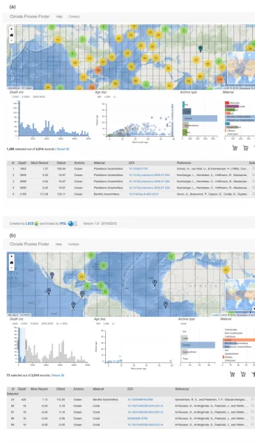
Figure 1.Web portal screen captures illustrating the search
crite-ria(a), the resulting maps(b), and the time-series plot(c).
0 50 100 150 200 250
0 5 10 15 20 25 30 35 40 45
1965 1970 1975 1980 1985 1990 1995 2000 2005 2010
Nu
mb
e
r
of r
e
cor
d
s
p
e
r
ye
ar
Nu
mb
e
r
of p
u
b
lic
ations
p
e
r
ye
ar
Year CE
Compiled records and publications per year
Figure 2.Number of publications and records in the database
ver-sus year of publication.
ocean, speleothem, tree) and material (e.g., carbonate, coral, etc.). A table of the available records is also displayed at the bottom of the screen (first 100 only). This table displays in-formation about the records (depth, age (most recent, oldest), archive, material, DOI, and the reference of the correspond-ing scientific paper). The DOI is hyper-linked to the Google Scholar search engine. The user can interactively filter the dataset by clicking or brushing over any of these charts or by dragging and zooming in and out of the map. Since all charts are interconnected, they will automatically be updated according to the filter selections. Figure 1b shows an exam-ple of this interactive filtering with the selection of ocean archive type near the surface (0–500 m). Accordingly, due to the cross-filtering functionality, all other charts and the table reflect only the proxies selected by these filters. This appli-cation also allows the user to display an interactive plot of the time series of the available isotopes by clicking on a map marker (see Fig. 1c for an illustration).
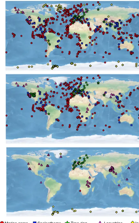
Marine cores Speleothems Tree-ring
cellulose Lacustrinecores Ice cores
Figure 3.Map indicating the position of archives with different
symbols representing the type of archive for datedδ18O (top)δ13C
(center) andδD records (bottom) available on the online portal.
Note that these maps only display the location of dated records, and stack and multi-sites composite records are not included.
Lastly, the user is able to download, in a zip file, the se-lected proxy data as CSV files and time-series plots by click-ing on the shoppclick-ing cart icon.
The Climate Proxies Finder application continues to evolve as new features are needed, such as adding a filter for proxy chronological information quality.
6 Results
0 50 100 150 200 250 300
-90 -80 -70 -60 -50 -40 -30 -20 -10 0 10 20 30 40 50 60 70 80 90
N
u
mb
er
o
f
co
mp
il
ed
reco
rd
s
Latitude (°N)
Ice core records Marine records Lacustrine records Speleothem records Tree ring records
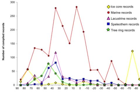
Figure 4.Diagram showing the distribution of ice core, tree-ring,
lacustrine, speleothem and marine records as a function of latitude (◦).
6.1 Geographical distribution of data and temporal resolution
This section briefly describes the status of the database for marine and terrestrial records (Fig. 3) and provides a synthe-sis of stable isotope data for each focus period.
A total of∼6400 records were collected from the NOAA and PANGAEA data repositories as well as from the internal LSCE database. About 3300 marine records were rejected, as they are not yet published. Following the settings of our online portal, we also isolated about 300δ18O andδ13C pub-lished records not dated (∼200 records) or containing no information about the core site elevation or depth (∼100 records). We thus accumulated about 1700δ18O records from
∼900 sites, about 900δ13C records from 450 sites, and about 230 δD records from 60 core sites (with 20 additional deu-terium excess records). When considering the different types of archives, we compiled about 1200 δ18O and∼700δ13C records from 600 marine sediment cores, 200δ18O and 75 δ13C speleothems records from 60 caves, 200 dated δ18O records from 50 ice cores (with about 60 additional dated δD datasets and∼20δ17O records), 60δ18O and 60δ13C la-custrine records (withδD datasets), and 85δ18O and 80δ13C records from tree rings.
Among all the 1900 collected marine records, about 850 do not present any information about the construction of their age model and about 950 records are associated with age model tie points or by default associated with an excellent chronology (e.g., modern corals), while most of the lacus-trine cores and speleothems are associated to chronological information. We also note that, when not considering tree-ring records, about 500 dated records do not present any sam-pling depth or distance scale. The absence of the age scale and/or chronological tie points clearly prevents any compar-ison with other records or with climate model output. Simi-larly, the absence of a depth scale prevents the detection of
potential sedimentary or chronological issues and therefore the correction with existing age models.
6.1.1 Geographical distribution
For each period of interest, although the number of compiled records is large enough, the geographic distribution of ma-rine cores is not homogenous, as 75 % of theδ18O andδ13C dated records are located in the Northern Hemisphere, with a maximum density in the northern subtropical band (Figs. 3 and 4). The Atlantic Ocean is the best documented (about half of all marine records). Most of the compiled records for the Indian, Pacific and Southern oceans come from sediment cores recovered on continental margins, because a part of the seafloor in the open ocean is deeper than the carbonate compensation depth in these basins (Berger and Winterer, 1974), and the sedimentation rate is particularly low in the large oligotrophic areas of the open ocean. This lack of suit-able core sites constitutes a critical limitation for the doc-umentation of the past open-ocean circulation and mecha-nisms affecting the entire Indian and Pacific basins, such as ENSO, latitudinal migrations of the ITCZ, and fluctuations in the thermohaline circulation, with possible formation of past North Pacific intermediate and deep water (Mix et al., 1999; Ahagon et al., 2003; Max et al., 2014) and storage of car-bon in the Southern Ocean (Skinner et al., 2010; Burke and Robinson, 2011). Vast areas remain virtually undocumented in the Indian, Pacific and Southern oceans. A large majority (about 90 %) of the records of the ocean database are based on foraminifera, while corals are much scarcer and only a few studies use mollusks or diatoms.
The distribution of continental records (Fig. 3) naturally depends on the position of caves, lakes, forests, and ice sheets and glaciers. Speleothemδ18O records are found on each continent, but with a very heterogeneous distribution. In fact, due to the distribution of caves presenting exploitable speleothems, several large areas (Russia and central Asia, northern and tropical Africa, Canada, central South America) remain undocumented, while the density of records is large in Europe, USA, Central America and China. While they have provided highly resolved records of regional climate variabil-ity (e.g., the monsoon and ITCZ, circum-Mediterranean con-tinental climate), speleothems do not provide a global cover-age. Lacustrine records are also very unevenly distributed, with very few dated isotopic records in South America, Africa, Russia and Australia, although these regions present numerous lakes.
0 50 100 150 200 250 300 350 400 7500
7000 6500 6000 5500 5000 4500 4000 3500 3000 2500 2000 1500 1000 500 500 1000 1500 2000 2500 3000 3500 4000 4500 5000
Number of records
D
e
p
th
(m
)
0
Ice cores
Lacustrine cores
Speleothems
Tree rings
Marine cores
Figure 5.Diagram showing the distribution of ice cores, tree-ring,
lacustrine, speleothem and marine records as a function of coring site elevation.
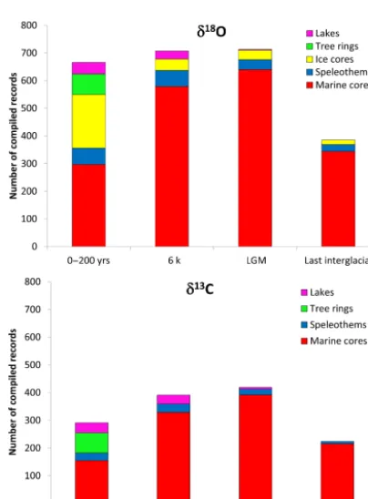
Figure 6.Diagrams showing the number ofδ18O andδ13C records
from marine and lake cores, speleothems, ice cores, and tree-ring cellulose for each PMIP time slice.
datasets (mainly δ13C records) are restricted to a few sites in Asia, South America, Siberia, Costa Rica and USA. This distribution of records implies that associated large-scale cli-mate reconstructions are somewhat constrained to Europe.
With respect to ice cores, 75 % of the compiledδ18O and δD are from Greenland and Antarctica. Few cores indeed were recovered from high-elevation ice caps and glaciers from the Andes, Alaska, Arctic Russia, Svalbard, Mount
Kil-Excellent
Good
Average
Marine cores
Speleothems
Tree-ring cellulose
Below average
Poor
Absent
Lacustrine cores
Ice cores Archive type
Age model quality evalua�on
Figure 7.Location of lacustrine (triangles), speleothems (squares)
and marine records (circles) where chronological information is available, and with quality flags for age model quality evaluation.
imanjaro and the high-latitude Canadian islands, close to Greenland (Fig. 3). We stress the fact that most published ice core records from Tibet spanning the past centuries are not available from open-access sources.
Contrary to the geographical distribution, the vertical dis-tribution of marine cores along the water column is relatively homogenous for the global ocean (Fig. 5), with more than 100 datasets in each of the 500 m thick layers from the sur-face down to 4000 m, while data are scarce below this level.
6.1.2 Temporal distribution
We now describe the distribution of records throughout the different periods of interest (Fig. 6). Marineδ18O andδ13C records are well represented over the four periods, with at least 200 records available for each of the time slices. How-ever, many marine sediment core tops are poorly dated, and thus the number of marine data delivering a robust character-ization of recent oxygen and carbon isotopic composition is limited. About half of the marine records have only one data point over the last 200 years (about 50 % of theδ18O records and 60 % of theδ13C records), and most of them have fewer than 10 data points over the last 200 years (∼65 % ofδ18O andδ13C records). When considering the other PMIP key periods, it appears that the distribution is similar for the MH (about 90 % of theδ18O and δ13C records have fewer than 10 data points), while the resolution is slightly better for the LGM (65 % ofδ18O and 70 % ofδ13C records have fewer than 10 data points) and for the large time interval assimi-lated here to the last interglacial (∼50 % records have fewer than 10 data points).
Marine records (reversed) Speleothems Lacustrine records Ice cores
MH-PD difference not significant
3 2 1 0.8 0.6 0.4 0.2 0 -0.2 -0.4 -0.6 -0.8 -1 -1.5 -2 -2.5 -3 0 5 10 15 20 25 -4 -3 -2 -1 0 1 2 3 4 -3 -2.5 -2 -1.5 -1
-0.8 -0.4 0.4
-0.2 0
-0.6 0.2 0.6 0.8
1 2 3
MH-PD�18O difference(‰)
MH-P D � 18O dif ference (‰ ) Fr ac ti on of th e total recor ds (%)
Figure 8.Map showing the location ofδ18O records spanning the
MH and PD with the symbols reflecting the type of source archive
and colors documenting the amplitude ofδ18O variations between
these two periods (MH-PD). The bottom figure shows the color scale as well as the fraction of records as a function of the MH-PD
δ18O anomaly. Note the non-linear scale forδ18O difference. The
δ18O difference from marine records was reversed for coherency
with the sign of changes of terrestrial records. Note that some proxi-mate core-sites may not be visible on the figure because of graphical overlaps.
As a result, although we compiled more than 200 speleothem δ18O records, none of the four key time slices selected by the PMIP project contains more than 60 records (30 for δ13C), due to the fact that many records span time inter-vals that are in between these time slices. Also, only three dated speleothem δ18O records span the entire time inter-val from the last interglacial period to present day, and only 14 records span both the LGM and the MH. In general, speleothem records have a better temporal resolution than marine records. For each of the four key periods, at least 60 % of the records display more than 10 data points. One diffi-culty arises from the fact that exceptionally long speleothem records such as the one obtained from the Hulu and Dongge caves records (Wang et al., 2001, 2005) have been obtained from the compilation of measurements performed on sev-eral speleothems/cores from one single cave. These multiple individual cores may present significant and varying offsets which can be identified over different periods of overlap (see Wang et al., 2001; Yuan et al., 2004). As a result, establish-ing a robust composite record allowestablish-ing calculation of anoma-lies between different past periods is particularly delicate for these archives. For this reason, we decided to keep the
indi-LIG-MH difference not significant Mar ine r ecor ds ( r ever sed) Speleot hem s I ce cor es
Fraction of the total recor ds (%) LIG-MH δ O d if fe re n c e (‰ ) 3 2 1 0.8 0.6 0.4 0.2 0 -0.2 -0.4 -0.6 -0.8 -1 -2 -3 0 5 1 0 1 5 2 0 2 5 3 0 - 4 - 3 -2 -1 0 1 2 3
-3 -2 -1
-0.8 -0.4 0.4
-0.2 0
-0.6 0.2 0.6
0.8
1 2 3
LIG-MH�18O difference (‰)
18
Figure 9.Same as Fig. 8 but for the difference between LIG and
MH values (LIG-MH).
LGM-MH difference not significant Marine records (reversed) Speleothems Ice cores LGM-M H � 18O dif ference (‰ ) Fraction of the total recor ds (%) 3 2 1 0 -0.3 -0.6 -0.9 -1.2 -1.5 -1.8 -2.1 -2.4 -2.7 -3 -4.5 -6 -8 0 5 10 15 20 25 -12 -10 -8 -6 -4 -2 0 2 4
-8 -6 -4.5 -3
-2.7 -2.1 -0.9
-1.8 -1.5
-2.4 1.2 -0.6 -0.3
0 1 2 3
LGM-MH�18O difference (‰)
Figure 10.Same as Fig. 8 but between the MH and the LGM
(LGM-MH).
vidual short datasets separated, following the way their au-thors published them, and we did not build long and continu-ous composite records. Therefore, composite records cannot be displayed in our LIG–MH comparison map (Fig. 9).
MH,∼40 for the LGM, and 14 concerning the LIG (13, 13 and 6 forδD, respectively). Only fiveδ18O records are con-tinuous from the LIG to the Holocene. Ice core records, how-ever, provide a wealth of information on the spatial and tem-poral variability of surface snow isotopic composition over the last decades, as about 140 of the ∼180 compiledδ18O dated records spanning the last 200 years exhibit at least 10 data points within this period (50 out of 55 dated records for δD and deuterium excess).
As the effect of burial on δ18O of fossil wood cellulose remains poorly known (Richter et al., 2008), we selected records exclusively based on living trees or timber wood. Consequently, the compiled records from tree-ring cellulose can only be used to monitor the climate fluctuations of the last millennium at the very best. We have identified ∼80 tree-ring cellulose δ18O records which cover the past 200 years (∼80 forδ13C). Most of the records have been pro-vided at seasonal to decadal temporal resolution.
Lacustrine cores are generally short and records generally span relatively limited time intervals. As a result, only the PD and MH are covered by a relatively large number of records (∼35δ18O, 30δ13C and∼135δD records for PD; 25δ18O, 30δ13C and∼45δD records for MH), while datasets span-ning the LGM and LIG are very scarce (30 when considering δ18O,δ13C andδD records).
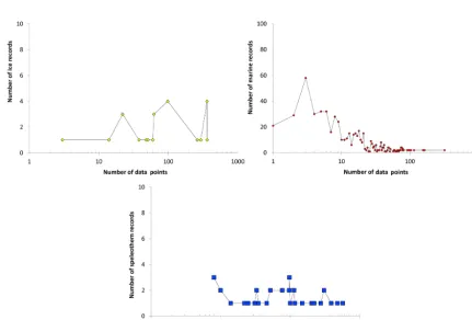
6.1.3 Datasets’ temporal resolution
Figure A1 (see Appendix A) shows the variety of temporal resolutions in the compiled records spanning the past 200 years (1800–2013 CE). Dating of marine sediment core tops remains a critical issue, due to alterations during the coring process as well as sediment reworking and bioturbation. In fact, the upper first centimeters are generally water-soaked and thus often lost or altered during the recovering of marine cores, which, in the case of moderate or low sedimentation rates, leads to the loss of material spanning the last hundreds or thousands of years. Additionally, bioturbation can alter the upper sediment down to 10 cm below the water–sediment in-terface (Boudreau, 1998). As a result, many core tops pro-vided as present-day references might actually reflect older conditions (from several centuries to a few millennia; Barker et al., 2007; Löwemark et al., 2008; Fallet et al., 2012). Solv-ing these issues might require a precise investigation of bio-turbation tracks in the upper layers of sediment cores and drastic improvement in the coring and analysis techniques, as suggested by the final conclusions of Keigwin and Guilder-son (2009): “Until we can directly radiocarbon date individ-ual foraminifera, the role of bioturbation will always be a problem in core top calibration studies.” These sedimentary issues are often accompanied by insufficient resolution and quality of the sediment core-tops dating procedure. In fact, present-day conditions are represented by only one data point in about half of the datasets, generally dated via linear ex-trapolation of deeper tie points. About 95 marine δ18O and
35δ13C records exhibit a decadal to annual resolution, gen-erally arising from corals (65 % of the records) with robust layer-counted annual chronology.
While chronology is not an issue for tree-ring cellulose records, the number of individual tree samples combined for each year can be a limiting factor. Several studies have in-vestigated the signal-to-noise ratio, and demonstrated the im-portance of combining at least 4–5 trees from a forest to ex-tract the common climate signal (e.g., McCarroll and Loader, 2004; Daux et al., 2011; Labuhn et al., 2014). The same issue arises for ice core records, especially for the past centuries, when the noise caused by processes such as wind scouring can be significant when compared to the small climatic signal (e.g., Fisher et al., 1985; Masson-Delmotte et al., 2015). As a result, the records resulting from stacks combining several ice cores from a given site have stronger climatic relevance than records based on individual ice cores. However, the non-polar ice cores experience their best dating on this period. The dating is usually based on the multi-proxy annual layer counting, which is based on the seasonal variations of insol-uble particles and the isotopic composition of ice. Moreover, the natural radioactive material decay of suitable radionu-clides (Pb210 for example) and the identification of promi-nent horizons of known age from radioactive fallout after at-mospheric thermonuclear test bombs (Cs137, Sr90, Am241) provide absolute reference horizons and are currently used in the Southern Hemisphere (Vimeux et al., 2008, 2009a, for example in the Andes).
Several recent speleothem and short ice core records ben-efit from annual layer counting, with an accurate chronol-ogy, but this is not systematic. Ice core datasets encompass a large proportion (∼70 %; 120 records) of highly resolved (decadal to annual) records, while this percentage is signif-icantly reduced for speleothems (about one-half of the 90 records spanning the last 200 years).
For the MH and LGM, marine records also have the low-est temporal resolution, as 80 % of these datasets exhibit four data points or less over the 5.5–6.5 ka interval, and none of the records are available with a resolution better than respec-tively 20 and 40 years (Figs. A2 and A3 in Appendix A). Ice core records spanning the MH and the LGM are rela-tively scarce (55 and∼50 datasets, respectively), and most of them exhibit decadal to centennial resolution. Speleothem records are slightly more abundant than ice core records (90 and 55 records for the MH and the LGM, respectively), with very variable resolution, from millennial to subdecadal. Speleothems and ice core records spanning the last inter-glacial are scarce (about 35 and 15 records, respectively; Fig. A4 in Appendix A) and only some of them present a cen-tennial resolution or better, while marine records are abun-dant, but most of them have millennial or lower temporal resolution.
the Holocene period, and few datasets cover the glacial pe-riod.
The present day is somewhat well resolved, as about 65 % of theδ18O andδ13C records spanning this time interval ex-hibit at least 10 data points. This trend is also observed for the MH, with about 65 % of the records presenting 10 or more data points.δD records appear to be much less well resolved, mostly because a large number of records originate from sur-face sediment studies based on dated core tops, resulting in a single data point. As a result, only 20 % on theδD records show at least 10 data points for the PD. This lower resolu-tion forδD is also verified for the MH, as none of the records present more than 10 data points.
6.1.4 Age model quality evaluation
Results from the evaluation of the quality of chronologies are highly variable from marine and lacustrine cores to speleothems (Fig. 7). The overall quality of age models for marine records is moderate. In fact, we note that most of the records published in the 20th century present a miss-ing or crude age model based on an insufficient number of AMS 14C dates, with a lack of reported technical informa-tion. Although this result is somewhat deceiving, the qual-ity of age controls has strongly improved during the last 15 years, thanks to better dating technologies and the growing awareness of the absolute necessity to publish robust and well-detailed chronologies to precisely reconstruct past cli-mate fluctuations.
Age models in speleothems are much better constrained, as most of the records present an “excellent” or “good” qual-ity flag. Speleothem records are indeed generally constrained by abundant U–Th dates and authors often provide highly detailed technical information. Age anomalies such as age reversals, outliers and hiatuses are nevertheless identified in many records. These anomalies can be caused by analytical issues (e.g., sample contamination, Th adsorption; Musgrove et al., 2001; Wainer et al., 2011) or natural factors occurring simultaneously or after sedimentation process (diagenetic al-teration). Hiatuses may be induced by climatic (e.g., severe droughts or permafrost impacts) or post-deposition (e.g., car-bonate dissolution) factors (Lachniet, 2009; Breitenbach et al., 2012).
The age models of lacustrine records are relatively good overall, with, however, largest discrepancies in the qual-ity of chronologies, depending on the dating technique. In fact, some lacustrine records are dated by counting an-nual/seasonal varves or laminations, leading to an excellent chronology. This dating technique is, however, generally lim-ited to relatively short records. Records providing longer signals (i.e., spanning several thousand years) are generally dated by AMS 14C dates. Similarly to what is observed for marine core dating, we note the possible lack of technical information in publications, as well as limited resolution of dates, which prevents the establishment of robust age
mod-els. Also, the potential adjustment applied to14C ages to cor-rect from radiocarbon reservoir and residence time effects is not systematically provided, nor is the presence of possible hiatuses.
6.2 Changes between PMIP key periods
δ18O from oceans and atmospheric water (and therefore con-tinental archives) vary in an opposite directions with climate fluctuations. We thus reversedδ18O fluctuations from ocean records in order to map coherent δ18O trends from all the different archives. However, we report the original values in the text. We report anomalies with respect to the MH for co-herency.
6.2.1 Changes between MH and present day
The relatively large number of datedδ18O datasets covering both the last 200 years (PD) and the mid-Holocene (MH) al-lows us to estimate possible offsets between these two pe-riods (MH-PD; ∼100 records from 70 sites; Fig. 8). We restrict the record selection to datasets presenting multiple data points for each of the two periods of interest, thus doc-umenting both the signal (average value) and noise (standard deviation). Results indicate a large dispersion of data, rang-ing from large positive to negative offsets, while most of the records depict in fact very similar values for the two periods. This feature reflects the spatial heterogeneity of the response to climate changes, making the establishment of large-scale patterns particularly difficult. In a given region, differences also emerge between records from different archives (e.g., opposite sign of changes in speleothem vs. lake records in eastern Europe). The average difference is low in ice cores, but the overall negative offset observed in ice cores indicates a polar cooling during the last 6 kyr, except around the Ross Sea in Antarctica. Particularly remarkable is also the positive anomaly from Chinese speleothems, commonly attributed to changes in Asian summer monsoon with a decrease in rain-fall amount through the Holocene (Cai et al., 2010). The stan-dard deviation of the data for the two periods of interest are, however, quite large in most cases. In fact, in the three types of archives, this noise is either of the same order or higher than the calculated PD–MH offset. As a result, the relatively weak isotopic change between these two periods is not sig-nificant in 2/3 of the records. Because we did not account for the analytical error associated withδ18O measurements (as this indication was missing in some of the datasets), we may underestimate the noise level and thus the number of records presenting an insignificant PD–MH offset.
6.2.2 Changes between the last interglacial and MH
two periods of interest. We observe more enriched continen-tal (more depleted marine)δ18O values for LIG than during the MH in∼20 records, suggesting relatively warmer condi-tions during LIG, with no apparent geographical trend. How-ever, about half of the LIG–MH anomalies are in the range of the natural standard deviation and thus cannot be consid-ered as statistically significant. Considering only the records presenting a significant offset nevertheless suggests warmer conditions (enriched continental and depleted marineδ18O) values during the LIG than MH.
Recent syntheses have shown contrasting results in tem-perature changes between the last interglacial period and present day (e.g., Otto-Bliesner et al., 2013), with positive temperature anomalies at both poles, but not occurring si-multaneously (Capron et al., 2014), and negative temperature anomalies in some tropical areas. Contrasting regional pat-terns are expected from the different orbital configurations. Several studies have also highlighted a large magnitude of climate variability during the LIG period (Cheddadi et al., 1998; Lototskaya and Ganssen, 1999; Hearty et al., 2007; Rohling et al., 2007; Pol et al., 2014).
6.2.3 Changes between the LGM and MH
Due to the limited amount of well-dated marineδ18O records covering both the LGM and present day with more than one data point, we compare the LGM and the MH for investigat-ing the isotopic amplitude of last termination (Fig. 10). The LGM–MH comparison reveals a significant negative (posi-tive) offset in almost all the terrestrial (marine) records, with only few speleothem and coral records showing the opposite trend, mostly in the subtropics, where they may reflect pre-cipitation or atmospheric circulation effects rather than local temperature variations.
The highest deglacial amplitude is recorded in high-elevation and polar ice core records, while the offset is less marked in oceans and speleothems. Marine datasets reveal a latitude-independent general amplitude of∼1.45 ‰ (1.55 ‰ when considering only foraminiferal records, with a similar average value for benthics and planktonics), out of which
∼1 ‰ is due to the change in land ice volume. In addi-tion, we observe specific regional patterns. Larger ampli-tudes are identified in marine records from the north and southeast Atlantic (about 1.7 ‰), which contrast with smaller amplitudes in the tropics (∼1.5 ‰) and maximum signals in the Mediterranean Sea (about 2.5 ‰). In this basin, this strong isotopic change is understood to reflect large SST deglacial warming and salinity changes induced by shifts in the regional atmospheric circulation (Bigg, 1994; Emeis et al., 2000; Hayes et al., 2005; Mikolajewicz, 2011). Statis-tics based on benthic foraminiferalδ18O records (including datasets presenting only one data point in the periods of in-terest) reveal that there is no influence of core site depth on the amplitude of the LGM to MH transition (R2=0.0029; n=180).
Ice cores records from high latitudes are all marked by a−3.3 to−7.7 ‰ δ18O shift, with, however, regional dif-ferences such as east–west gradients in both Greenland and Antarctica. Such regional differences may be induced by changes in ice sheet topography and different amplitudes of surface elevation changes at different locations (e.g., Vinther et al., 2009). Similar mechanisms may be at play in Antarc-tica, but these remain poorly documented (e.g., Masson-Delmotte et al., 2011b). There is also evidence for regional differences in the response of Antarctic temperature to cli-matic changes (Turner et al., 2005; Steig et al., 2009; Steig and Orsi, 2013). The larger amplitude of glacial–interglacial isotopic changes in West Antarctica has been suggested to re-flect regional processes coupling the Southern Ocean, sea ice extent and atmospheric heat transport (WAIS Divide Project Members, 2013). It is worth noting that Andean ice cores spanning the last glacial–interglacial transition show a sim-ilar deglacial isotopic shift (Vimeux, 2009b). The water sta-ble isotopic composition in those ice cores is likely reflecting precipitation changes at the regional scale, and such a similar deglacial structure is explained by simultaneous cold condi-tions in the high latitudes and wetter condicondi-tions in the Andes (Vimeux et al., 2005; Chiang and Koutavas, 2004).
Different patterns emerge from speleothem records cov-ering the LGM and MH, as only half of the datasets are marked by a more depleted glacialδ18O level. Depending on the location, speleothem calciteδ18O may reflect paleotem-perature and/or past changes in the atmospheric water cy-cle (including precipitation and circulation). Additional site-specific factors (cave microclimate, mixing and evaporation of source waters through the soil and the epikarst, kinetic fractionation during carbonate precipitation) may also influ-ence the signal (Lachniet, 2009). Regional effects may also be at play in the western Middle East, where speleothem records can be directly influenced by changes in the Mediter-ranean or the Black Sea, which had diverging oceanographic evolutions between the LGM and the MH, with the open-ing of the Bosphorus Strait. Individual records must therefore be understood in their own regional environmental context, a feature also evidenced by different amplitudes of change aris-ing from different source archives. Thus, Figs. 8–10 might be considered as an inventory of the available datasets, rather than a cartography of the amplitude of climatically relevant signals, expected to be representative of the amplitude of an-nual mean precipitation or sea water isotopic composition changes.
7 Conclusions, recommendations and perspectives
datasets provided by authors. This effort would be made eas-ier if the data and publication information (core site spec-ifications, references, article title and abstract) were stored in individual CSV (comma-separated value) text files, rather than within files specifically designed for spreadsheet soft-ware (e.g., Microsoft Excel/Apache OpenOffice), sometimes containing several spreadsheets, that may not be readable by automated data extraction programs. We also think that building a fixed disposition for datasets constitutes a prelim-inary step and that it is essential for the existing and future data depositories to find an agreement for an harmonized dis-position, structure, and labeling for metadata and age mod-eling data storage. Some projects are following a promis-ing philosophy of homogenously structured metadata (e.g., LiPD; McKay and Emile-Geay, 2016). We highly encourage these constructive initiatives, as it is becoming urgent for the paleoclimate research community to definitively adopt a uni-versal file format and metadata disposition and to define the type of contents to be included, before starting to compile data, as this will otherwise lead to a high risk of incompati-bility or of conflicting information from different sources or projects. Adopting this universal format will, however, ne-cessitate a clear agreement between data producers, users, and compilers, as it requests at the end a unique structure compatible with all types of archive and proxies, which may lead to some complications due to the variable number of parameters to be included for each proxy and archive. If a universal standard format is definitively adopted, the conver-sion of our metadata spreadsheet into a hierarchical struc-tured may be relatively easy and fast.
Divergences in data units also constitute a major obsta-cle for automated extraction, intercomparison of records, and model–data comparisons. An illustrative example is the use of various time units (years CE, years or before 2000 CE, years before 1950 CE, kiloyears BP, and million years BP). The establishment of standard time units for paleoclimatol-ogy such as the use of “ka” (calendar kiloyears before 1950) would avoid errors and homogenization of future datasets. Several discrepancies also exist with respect to the geograph-ical coordinates of core sites. Although the most common format found in the literature is DMS (degrees, minutes, sec-onds; e.g., 25◦22034 N, 38◦16043 W), it is not supported by most mapping programs. Here, we converted all the geo-graphical coordinates into decimal degrees. We again highly encourage the adoption of a standard notation, with the sys-tematic presence of the decimal degree version of the coordi-nates; we observe that an increasing number of authors now provide both DMS and decimal formats.
Gathering information about the age models was a par-ticularly critical step of the construction of this database, in particular for the inclusion of lacustrine and deep-sea cores as well as speleothems. We highly encourage authors to sys-tematically provide both depth and age scales as well as a comprehensive description of the methodology used to es-tablish the age scale, when available. While our earlier
com-ment was centered on deep-sea cores, the same features ap-ply for the description of lake sediment cores, ice cores and speleothem chronologies. Even if the methodology devel-oped for the successive chronologies of deep ice cores is usu-ally precisely documented, no standardized reporting proto-col exists for ice cores from tropical and temperate glaciers. There is, however, no existing standard procedure for the de-scription of age models. The available information is often fragmented, with missing information (raw AMS14C dates, calibration program/curve used to compute calendar ages, species used for analysis, amount of material measured, ma-rine reservoir ages, tie points, identification of hiatuses in speleothems etc.). A standardized format including all the information related to the establishment of the age models would be a major step forward. Finding a common structure might, however, constitute a fastidious task, particularly be-cause the samples dating techniques are radically different for the different types of archives. A first step would con-sist in finding a standard structure to be adopted for AMS
14C measurements performed, for instance, on speleothems,
marine and lacustrine cores. Many old records are associ-ated with very limited information concerning their chronol-ogy, which prevents any attempt to reproduce the age model. Consequently, it is becoming necessary to adopt a common format which would be interoperable between the different data repositories and would include all the necessary infor-mation to recalculate age models. For age models based on AMS14C dating, we suggest that the following information should become mandatory:
– core ID;
– sample ID, lab name;
– sample depth with indication of any depth correction;
– type of material analyzed, including species;
– indication of sedimentary disturbances (hiatuses, tur-bidites, tephras, etc.) and their corresponding depth;
– AMS14C ages and the associated error;
– calibrated ages and the associated error;
– program/calibration curve used for14C dates calibra-tion;
– reservoir age for marine cores, and the associated un-certainties;
– dates removed from the construction of the age model and the reason why they were eliminated.
We have noticed a clear improvement in the quality of age models and in dating technique description during the last two decades, and most of the low quality chronologies were published more than 20 years ago. This improvement in age models is particularly critical with respect to the sequences of events during fast transient climate reorganizations. In fact, previous studies have shown that many past major climate changes involved abrupt responses (e.g., de Menocal et al., 2000; Genty et al., 2006; Carlson et al., 2007; Zuraida et al., 2009; Clark et al., 2012; Rach et al., 2014) as well as short delays between different proxy records and regions, like the vigorously debated date and triggering of the onset of Ter-mination I (Schaeffer, 2006; Stott et al., 2007; Koutavas and Sachs, 2008; Smith et al., 2008; Bromley et al., 2009; Clark et al., 2009; Shakun et al., 2012; Parrenin et al., 2013). In this context of successive rapid climatic events, and keeping in mind the growing interest on transient climate simulations, it thus becomes necessary to have a large amount of pre-cisely dated and well-defined records. Reservoir ages remain a critical issue in paleoceanography, as do their uncertain-ties. Many efforts have been deployed during the last decade to better estimate reservoir ages. Several publications have also suggested changes in reservoir ages between glacial and interglacial periods (e.g., Waelbroeck et al., 2001; Bondevik et al., 2006; Sikes and Guilderson, 2013). In this context, the age model of many old records may be outdated, and even considered to be wrong. Unfortunately, the lack of informa-tion concerning the construcinforma-tion of these initial age models makes the construction of an updated age model virtually im-possible. In this study, we did not aim to evaluate the accu-racy of published reservoir ages, which remain sometimes vigorously debated. We encourage authors of publications to systematically justify their choice of a reservoir age, to de-scribe the associated uncertainties, together with the detailed age model information.
Our database may in the future allow the implementation of statistical age models built on the existing age markers. Reporting the exact number of source records for tree rings and ice cores is also important with respect to the signal to noise issue; this is not always a standard practice.
Our software tool was designed to make the update of the database user-friendly and easy in order to allow future extension. Indeed, major synthesis efforts as the MARGO project (Waelbroeck et al., 2009) are time-limited (MARGO only includes records published prior to 2005). Options for an automatic update include regular browsing of new pub-lished data, but we highly encourage authors to upload their new data in our database using the user-friendly interface on the online platform. This constitutes a fast and easy way to disseminate new data and increase their visibility, and a unique opportunity for the scientific community to access and exploit newly published datasets. This allows “data pro-ducers” to easily compare their records with other existing records in a given area or at the global scale, and climate
modelers to access easily the data, and to the source refer-ences and their authors.
In the future, and if manpower resources are available, the database and web interface could be easily opened to other proxies (paleotemperature proxies and nitrogen iso-topes for seawater, CO2and CH4 from ice cores, tree-ring
width and boreholes, pollen, circulation tracers such as14C and Pa/Th, etc.) of past and future datasets. We also hope that our database, associated with current and upcoming projects focusing on time-series age control (INTIMATE PROJECT, COST Action ES0907) and chronological data managing (Mulitza and Paul, 2013), will in the future facilitate the use of paleoclimate datasets for data comparison and integration into models with an homogenous and robust chronological frame. This is expected to strengthen the use of proxy in-formation for model–data comparisons, a topic promoted in the Stable Water Isotope Intercomparison Group (SWING) and the isotope modeling working group of the Paleoclimate Modelling Intercomparison project, with the potential to bet-ter document projections (Schmidt et al., 2014).
8 Data availability
Appendix A: Statistical analysis – estimation of the significance of the offset between PMIP time slices
The significance of the difference between two different PMIP time slices (AandB) was assessed by simply com-paring the offset between the average isotopic value of these two periods (AandB) to the average value of the standard deviations of the isotopic record for each of the two periods (σ Aandσ B).
A−B⇐⇒σ A+σ B
2
Figure A2.Same as Fig. 1 but for the mid-Holocene (5.5–6.5 ka). Note the different vertical scales.