https://doi.org/10.5194/os-14-999-2018
© Author(s) 2018. This work is distributed under the Creative Commons Attribution 4.0 License.
Circulation of the Turkish Straits System under interannual
atmospheric forcing
Ali Aydo˘gdu1,2,3, Nadia Pinardi4,5, Emin Özsoy6,7, Gokhan Danabasoglu8, Özgür Gürses6,9, and Alicia Karspeck8 1Science and Management of Climate Change, Ca’ Foscari University of Venice, Venice, Italy
2Centro Euro-Mediterraneo sui Cambiamenti Climatici, Bologna, Italy 3Nansen Environmental and Remote Sensing Center, Bergen, Norway
4Department of Physics and Astronomy, University of Bologna, Bologna, Italy 5Istituto Nazionale di Geofisica e Vulcanologia, Bologna, Italy
6Institute of Marine Sciences, Middle East Technical University, Erdemli, Turkey 7Eurasia Institute of Earth Sciences, Istanbul Technical University, Istanbul, Turkey 8National Center for Atmospheric Research, Boulder, CO, USA
9Alfred Wegener Institute for Polar and Marine Research, Bremerhaven, Germany Correspondence:Ali Aydo˘gdu ([email protected])
Received: 16 January 2018 – Discussion started: 31 January 2018
Revised: 31 May 2018 – Accepted: 25 July 2018 – Published: 11 September 2018
Abstract. A simulation of the Turkish Straits System (TSS) using a high-resolution, three-dimensional, unstruc-tured mesh ocean circulation model with realistic atmo-spheric forcing for the 2008–2013 period is presented. The depth of the pycnocline between the upper and lower lay-ers remains stationary after 6 years of integration, indicat-ing that despite the limitations of the modellindicat-ing system, the simulation maintains its realism. The solutions capture im-portant responses to high-frequency atmospheric events such as the reversal of the upper layer flow in the Bosphorus due to southerly severe storms, i.e. blocking events, to the ex-tent that such storms are present in the forcing dataset. The annual average circulations show two distinct patterns in the Sea of Marmara. When the wind stress maximum is localised in the central basin, the Bosphorus jet flows to the south and turns west after reaching the Bozburun Peninsula. In con-trast, when the wind stress maximum increases and expands in the north–south direction, the jet deviates to the west be-fore reaching the southern coast and forms a cyclonic gyre in the central basin. In certain years, the mean kinetic energy in the northern Sea of Marmara is found to be comparable to that of the Bosphorus inflow.
1 Introduction
The Turkish Straits System (TSS) connects the Marmara, Black and Mediterranean seas through the Bosphorus and Dardanelles straits. The near-surface layer of low salinity wa-ters originating from the Black Sea enwa-ters from the Bospho-rus, flowing west and exiting into the Aegean Sea at the Dar-danelles. The deeper, more saline waters of Mediterranean origin enter from the Dardanelles in the lower layer and eventually reach the Black Sea through the undercurrent of the Bosphorus. The strongly stratified marine environment of the TSS is characterised by a sharp pycnocline positioned at a depth of 25 m (Ünlüata et al., 1990). The complex to-pography of the Sea of Marmara consists of a wide shelf in the south, a narrower one along the northern coast and three east–west deep basins separated by sills, connected to the two shallow, elongated narrow straits providing passage to the ad-jacent seas at the two ends, as shown in Fig. 1.
filer (ADCP) measurements at the straits (Özsoy et al., 1988, 1998; Altıok et al., 2012; Jarosz et al., 2011b, a, 2012, 2013). Updated reviews of TSS fluxes based on combined data have been provided by Schroeder et al. (2012), Özsoy and Altıok (2016), Sannino et al. (2017) and Jordá et al. (2017).
The hydrodynamic processes of the TSS extend over a wide range of interacting space scales and timescales. The complex topography of the straits and property distributions have resulted in hydraulic controls being anticipated in both straits (Özsoy et al., 1998, 2001), which can only partially be demonstrated by measurements at the northern sill of the Bosphorus (Gregg and Özsoy, 2002; Dorrell et al., 2016). Hydraulic controls have since been found by modelling at the southern contraction-sill complex and the northern sill, confirming a unique maximal exchange regime adjusted to the particular topography and stratification (Sözer and Öz-soy, 2017a; Sannino et al., 2017). These findings support the notion that the Bosphorus is the more restrictive of the two straits in controlling the outflow from the Black Sea to the Mediterranean. The analysis of moored measurements by Book et al. (2014) demonstrated this and indicated a more re-strained sea level response transmitted across the Bosphorus than in the Dardanelles.
Improvements in modelling have provided a better sci-entific understanding of the TSS circulation, and they can now address the complex processes characterising the sys-tem. The initial step in this formidable task is to construct separate models of the individual compartments of the sys-tem, which are the two straits and the Marmara basin. The first simplified models of the Bosphorus were by Johns and O˘guz (1989), who solved the turbulent transport equations in 2-D and found a two-layer stratification to develop. Sim-plified two-layer or laterally averaged models of the Dard-anelles and Bosphorus were later developed by O˘guz and Sur (1989), Stashchuk and Hutter (2001) and O˘guz et al. (1990), respectively, while Hüsrevo˘glu (1998) introduced a 2-D reduced gravity ocean model of the Dardanelles in-flow into the Sea of Marmara. Similar 2-D laterally aver-aged models (Maderich and Konstantinov, 2002; Ilıcak et al., 2009; Maderich et al., 2015) and 3-D models (Kanarska and Maderich, 2008; Öztürk et al., 2012), which were of limited extent, have been used to construct simplified solutions for the Bosphorus exchange flows. Bosphorus hydrodynamics were extensively investigated by Sözer and Özsoy (2017a) using a 3-D model with turbulence parameterisation under idealised and realistic topography with stratified boundary
Very few studies have attempted to model the circulation in the Sea of Marmara, even as a stand-alone system exclud-ing the dynamical influences of the straits and atmospheric forcing. Chiggiato et al. (2012) modelled the Sea of Marmara using realistic atmospheric forcing and open boundaries at the junctions of the straits with the sea, indicating surface cir-culation changes in response to changes in the strength and directional pattern of the wind force.
Similarly, the interannual variability of the Sea of Mar-mara has been examined by Demyshev et al. (2012) using open boundary conditions at the strait junctions in the ab-sence of atmospheric forcing. They reproduced the S-shaped jet current traversing the basin under the isolated conditions of a net barotropic current, which with appropriate parame-terisation successfully preserved the sharp interface between the upper and lower layers when the model steady state was reached after 18 years of simulation. The S-shaped upper layer circulation of the Sea of Marmara predicted by Demy-shev et al. (2012) appears similar to what Be¸siktepe et al. (1994) found in summer, when wind forcing is at its min-imum or at least close to being in a steady state. An anti-cyclonic pattern has generally been identified in the central Sea of Marmara, like the cases reported by Be¸siktepe et al. (1994).
The challenges of modelling the entire TSS domain were recently undertaken by Gürses et al. (2016). The effects of at-mospheric forcing were considered, excluding the effects of the net flux through the TSS. The study used an unstructured triangular mesh model, the Finite Element Sea-Ice Ocean Model (FESOM), with a high horizontal resolution reaching about 65 m in the straits in the horizontal. The water column is discretised by 110 vertical levels.
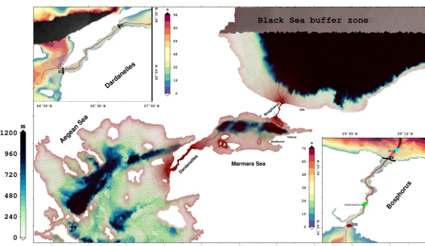
Figure 1.Bathymetry of the Turkish Straits System and the whole model domain. Bathymetry of the Bosphorus and Dardanelles straits is detailed in the small panels. The colours represent the depth. The colour bar scales are different for the straits and the whole domain. A triangular mesh is overlaid with red for the entire domain and with grey for the straits in small panels. The thalweg used to display the cross-section throughout the TSS is represented by the black line. The grey shaded area in the Black Sea functions as a buffer zone and is described in the text. Cross-sections at the boundaries of the straits are used for volume flux computations. NB, SB, ND and SD in the small panels are northern Bosphorus, southern Bosphorus, northern Dardanelles and southern Dardanelles, respectively. In the Bosphorus panel, the green and cyan squares show the locations of the contraction and northern sill, respectively. Finally, the red square B1 indicates the middle of the Sea of Marmara exit of the Bosphorus strait.
lower layer in the Bosphorus being blocked. The most sig-nificant finding was the non-linear sea level response, which deviated widely from the linear response predicted by the stand-alone Bosphorus model of Sözer and Özsoy (2017a).
Stanev et al. (2017) approached the challenge by using an unstructured mesh model. The model covers the entire Black Sea and is seamlessly linked to the TSS and the northern Aegean Sea with open boundaries in the south and uses re-alistic atmospheric forcing. The focus is on the transport at the straits and the resulting dynamics of the Black Sea. Re-garding the TSS, the results support the notion of multiple controls of the barotropic flow. They were also able to sim-ulate short-term events such as severe storm passages. How-ever, in a high-resolution model of the TSS, the Courant– Friedrichs–Lewy (CFL) condition (Courant et al., 1967) re-stricts the time step to a few seconds with explicit schemes. As a solution, Stanev et al. (2017) used an implicit advec-tion scheme for transport to handle a wide range of Courant numbers (Zhang et al., 2016) while satisfying the stability of the solution. However, the computational burden of us-ing an implicit scheme imposed a coarser model resolution with 53 vertical levels at the deepest point of the Black Sea. We note that this limitation may, particularly in the Bospho-rus, lead to excessive vertical mixing or a widened interface
thickness, which are crucial for the intrusion of the Mediter-ranean origin water into the Black Sea. This can be seen in their Fig. 11c and d, for example.
Another recent study by Ferrarin et al. (2018) presents the tidal dynamics in the TSS which is seamlessly included in a model domain covering whole Black Sea – Mediter-ranean system. They use a barotropic version of SHYFEM (Umgiesser et al., 2004) to provide the hydrodynamical back-ground to the tidal analysis.
In our work, we simulate the complete TSS with a high-vertical-resolution unstructured grid model forced by com-plete heat, water and momentum fluxes. A long-term 6-year simulation is used to analyse the combined response of the Sea of Marmara to atmospheric forcing and strait dynamics. The questions addressed in this paper are
– What is the mean Sea of Marmara circulation and its variability in a long-term simulation?
– What are the effects of the atmospheric forcing on the Sea of Marmara dynamics and circulation?
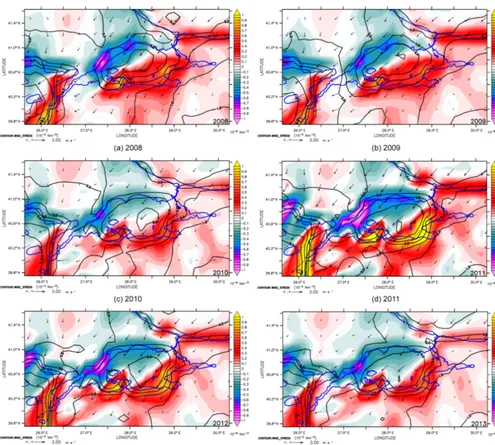
Figure 2.Annual mean of wind velocity (ms−1, arrows), wind stress (10−2Nm−2, black contours) and wind stress curl (10−6Nm−3, shades) in the Sea of Marmara for each year from 2008(a)to 2013(f). The coastline is overlaid in blue.
level differences along the TSS are demonstrated. The re-sulting volume transport through the straits, and the kinetic energy and circulation in the Sea of Marmara, are presented. Finally, in Sect. 4, we summarise and discuss the results.
2 Model setup
Models for solving the dynamical equations for an un-structured mesh using finite element or finite volume meth-ods have been implemented for many idealistic applications (White et al., 2008; Ford et al., 2004) and in realistic coastal ocean studies (Zhang et al., 2016; Federico et al., 2017;
Stanev et al., 2017). An obvious advantage of using an un-structured mesh model is the varying resolution, which al-lows for a finer mesh resolution in coastal areas than in the open ocean. The general ocean circulation model used in this study is FESOM. FESOM is an unstructured mesh ocean model using finite element methods to solve hydro-static primitive equations with the Boussinesq approximation (Danilov et al., 2004; Wang et al., 2008). We use the initial implementation of Gürses et al. (2016).
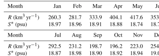
Table 1.Monthly Black Sea river discharge (R) and salinity relaxation values (S∗).
Month Jan Feb Mar Apr May Jun
R(km3yr−1) 260.3 281.7 333.9 404.1 417.6 353.6
S∗(psu) 18.97 18.96 18.91 18.88 18.74 18.74
Month Jul Aug Sep Oct Nov Dec
R(km3yr−1) 292.5 231.2 198.7 196.2 223.0 254.2
S∗(psu) 18.87 18.98 18.90 18.92 18.94 19.02
Sea of Marmara, the resolution is always finer than 1.6 km and is not coarser than 5 km in the Black Sea and the Aegean Sea. The water column is discretised by 110 verticalzlevels. The vertical resolution is 1 m in the first 50 m depth and in-creases to 65 m at the bottom boundary layer in the deepest part of the model domain.
Model equations and parameters are documented in Ap-pendix A. The current model implementation considers closed lateral boundaries. Therefore, volume and salinity conservations are imposed to prevent drifts in the tracer fields. Our approach for volume and salinity conservations is described in Appendix B.
The experiment detailed below was conducted over 6 years, commencing on 1 January 2008 and continuing un-til 31 December 2013. The initial fields were obtained af-ter a 3-month integration of a lock-exchange case, which was initialised from different temperature and salinity pro-files in the basins of the Black, Marmara and Aegean seas (Gürses et al., 2016; Sannino et al., 2017). Fine mesh resolu-tion and energetic flow structures in the straits require small time steps so the CFL condition is not violated. The time step is thus set to 12 s throughout the integration. The simulation was forced by atmospheric fields provided by European Cen-tre for Medium-Range Weather Forecasts (ECMWF) with 1/8◦ resolution. The forcing data cover the whole experi-ment period with a time frequency of 6 h. Precipitation data are obtained from monthly CPC Merged Analysis of Precip-itation (CMAP; Xie and Arkin, 1997) and interpolated to the ECMWF grid as daily climatology.
The annual means of wind, wind stress and wind stress curl for the simulation period are shown in Fig. 2. Wind stress,τ, is calculated as
τ =ρ0Cd|uwind|uwind, (1) whereCdis the drag coefficient anduwindis the wind veloc-ity. The annual mean wind fields are northeasterlies which were strongest in 2011.τ was higher than 0.04 Nm−2in the central north Sea of Marmara in 2009. It then expands in a north–south direction, exceeding 0.05 Nm−2 in the central basin, in 2011, and then weakens again in 2013. The wind stress curl is a dipole shaped by the northeasterlies and is negative in the north and west, and positive in the south and
east of the Sea of Marmara. In 2011, the wind stress curl in the coastal zones was more intense than in the other years.
A surface area of 22 693 km2 north of 42.5◦N in the Black Sea functions as a buffer zone (the grey shaded area in Fig. 1). This zone is utilised to provide required water fluxes for a realistic barotropic flow through the Bosphorus. The model is forced by climatological runoff in the Black Sea, which is essential to generate realistic sea level differ-ences between the compartments of the system (Peneva et al., 2001). The monthly runoff climatology for water fluxes was obtained from Kara et al. (2008) and is the same for all the 6 years. The surface salinity at the buffer zone was relaxed to a monthly climatology, computed from a 15-year simulation by the Copernicus Marine Environment Monitoring Service Black Sea circulation model (Storto et al., 2016). The salin-ity relaxation time is approximately 2 days. Although this is a strong constraint, it is required to prevent the surface salin-ity from decreasing in the buffer zone due to the excessive amount of fresh water input. The climatological values used for runoff and salinity relaxation are shown in Table 1.
Here, we note again that the model having closed lat-eral boundaries requires a correction for the water and mass fluxes which we discuss in Appendices A and B. Very briefly, the access or deficit of the water fluxes is redistributed to the surface model nodes weighted by the corresponding element area. Since a runoff climatology is inserted in the Black Sea to maintain the sea level difference along the system, the cor-rection will enforce the volume conservation. This method was also used by Gent et al. (1998) for a climate global model. Another method was explored by Gürses et al. (2016) where the correction was applied only in the Aegean area but salinities became too high and the salinity profile of the simulation became unrealistic.
3 Results
Figure 3.Monthly averaged net heat (blue) and water (black) fluxes in the Sea of Marmara, along with evaporation (dashed) and precip-itation (dotted). Runoff is zero in the Sea of Marmara. The blue vertical axis (right) is for heat flux and the black vertical axis (left) for water fluxes. Water flux correction described in Appendix A is shown in red. The 6-year mean values of fluxes are marked on the figures and shown in legends.
are analysed. Although we will include results demonstrating the response of the system to daily atmospheric events, we focus on the interannual changes in the TSS. Therefore, we consider only annual means in time averages. The computed time averages for the simulation are for the period 2009– 2013, as the first months of 2008 are considered as an initial spin-up period.
3.1 Surface heat and water fluxes
The monthly averages of water fluxes and net heat flux are shown in Fig. 3a for the whole domain and Fig. 3b for the Sea of Marmara. The mean runoff, evaporation and precipitation in the whole domain are 278.1, −131.5 and 70.8 km3yr−1, respectively. The resulting net water flux into the ocean is therefore 226.4 km3yr−1which is balanced by the correction term (see Appendix A) shown in red in Fig. 3a. As a result, the model volume is conserved.
In the Sea of Marmara, runoff is identically zero (Fig. 3b). Mean evaporation and precipitation are−8 and 6.8 km3yr−1, respectively. The water flux correction applied in the Sea of Marmara is −15.9 km3yr−1. This means there is a net surface flux loss in the Sea of Marmara of about
−17.1 km3yr−1. The total water budget of the Sea of Mar-mara will be further discussed in Sect. 3.3.
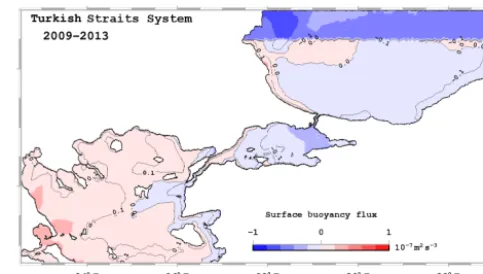
Figure 4.Mean of surface buoyancy fluxes for 2009–2013. A neg-ative value is the buoyancy flux down into the ocean.
The net heat flux in the Sea of Marmara is calculated in the range of−123.3 to 138.4 W m−2with minimums and maxi-mums in December–January and May–June, respectively.
The daily buoyancy fluxes were averaged between 2009 and 2013, and are shown in Fig. 4. The buoyancy flux was computed using the following formula:
Qb=
gα ρ0Cw
QH−βS0gQw, (2) whereαandβare thermal expansion and haline contraction coefficients (McDougall, 1987),QHis the heat flux (positive towards the ocean),Cwis the specific heat capacity,S0is the surface salinity, andQwis the water flux.
The Black Sea and the Sea of Marmara gain buoyancy ex-cept for a small area near their western coasts (Fig. 4), while the Aegean Sea has a buoyancy loss except near the Dard-anelles exit and the Anatolian coast. The average buoyancy flux changes between−7×10⁻⁸and 3.4×10⁻⁸m2s−3over the domain. It does not show significant spatial differences interannually, but the gradient between the Aegean and Black seas was stronger in 2011 than in the other years (not shown). 3.2 Water mass structure and validation
Figure 5.The mean sea surface salinity for 2009–2013. Contours are overlaid with a 1 psu interval.
are colder and continuously modified by the Dardanelles in-flow after the initialisation, as can be seen in Fig. 7, in which the volume temperature has a negative trend and salinity a positive one. We argue that this is due to initialisation adjust-ment and the closed boundary conditions. Salinity is com-pletely mixed in the Sea of Marmara below 100 m depth.
In the Bosphorus, Altıok et al. (2012) reported a cold tongue in June–July between 1996 and 2000, with a temper-ature of about 11–12◦C, extending to the Sea of Marmara. This cold tongue is reproduced in the simulation (Fig. 6b) and emerges as a cold intermediate layer (CIL) at the posi-tion of the halocline.
The mean sea surface temperature in the Sea of Marmara fluctuates between 4.4 and 28.3◦C (Fig. 7). Surface mean salinities are lower in the spring and early summer than at other times of the year. The volume mean temperature de-creases from 11 to 9–10◦C and varies seasonally.
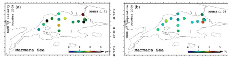
Three datasets of in situ conductivity–temperature–depth (CTD) observations were collected by R/V Bilim-2 from the Institute of Marine Sciences (IMS/METU1) on 4– 11 April 2008, 1–4 October 2008 and 18–23 June 2013 are used to validate the simulation.
Figure 8 shows the spatial distribution of the salinity and temperature RMS errors in the first 50 m of the water col-umn in October 2008. The error is higher in the eastern Sea of Marmara close to the Bosphorus. The mean RMS errors of temperature and salinity are listed in Table 2. The errors are similar in April and October 2008 but notably increase after 6 years of integration in June 2013, which can be expected after such a long integration and, spatially, the errors are this time higher on the Dardanelles side of the Sea of Marmara than on the Bosphorus side. The RMS error is larger than 1Two datasets are from European SESAME-Southern Euro-pean Seas: Assessing and Modeling Ecosystem Changes Integrated Project/FP6. The other dataset is from the subsequent PERSEUS: Policy-oriented marine Environmental Research for the Southern European Seas, funded by the EU under the FP7 theme “Oceans of Tomorrow” (OCEAN.2011-3 grant agreement no. 287600).
those found in operational models of the Mediterranean Sea (Oddo et al., 2009), but this is due to a thermocline and halo-cline vertical shift, as shown in Fig. 9a. The vertical mix-ing and the missmix-ing interannual variability of the Black Sea runoff probably account for this. The model performs sub-stantially better at the surface and below 30 m in depth than it does at the depth of the interface between the upper and lower layers of around 20 m (Fig. 9b). Temperature RMS errors are highest around the seasonal thermocline in June 2013, while at the same level as the halocline in the other 2 months.
3.3 Sea level and volume fluxes through the straits
The time mean of the sea surface height across the system is shown in Fig. 10 for the 2009–2013 period. The SSH is approximately 0.12 m in the Black Sea and−0.12 m in the Aegean Sea. In the Sea of Marmara, SSH is higher in the western basin. The differences between the two ends of the Bosphorus are approximately 0.18 m and in the Dardanelles are about 0.11 m.
Moller (1928) measured the sea level differences between the two ends of the Dardanelles and the Bosphorus as 7 and 6 cm, respectively. Gunnerson and Ozturgut (1974) and Büyükay (1989) found the sea level difference in the Bospho-rus to be 35 cm for the 1966–1967 period and 28–29 cm for 1985–1986 period, respectively. Bogdanova (1969) gave a sea level difference of 42 cm between the northern Black Sea (Yalta) and southern coast of Turkey (Antalya) with high sea-sonal variability. Alpar et al. (2000) suggested a mean sea level difference of 55 cm between the Black Sea entrance of the Bosphorus and the Aegean entrance of the Dardanelles for the 1993–1994 period. We cannot assess the accuracy of our model against these values in the literature with such a wide range of variability.
Figure 6.Annual mean of(a)salinity and(b)temperature for 2013 along the thalweg.
Table 2.Mean RMS of salinity and temperature error with respect to CTD measurements in April and October 2008 and June 2013.
Apr 2008 Oct 2008 Jun 2013
psu/◦C Salinity Temperature Salinity Temperature Salinity Temperature
1.34 0.77 1.71 1.09 3.18 2.09
Figure 7.Daily time series of mean sea surface temperature (SST), mean sea surface salinity (SSS), volume mean temperature (VT) and volume mean salinity (VS) in the Sea of Marmara. Temperature and salinity are shown in black and red, respectively.
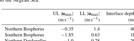
Table 3.Along-strait maximum velocity for the upper layer (UL) and lower layer (LL) and interface depth in each strait exit. Units are in m s−1and metres for the velocity and depth, respectively. A negative value indicates the flow in the direction from the Black Sea to the Aegean Sea.
UL|umax| LL|umax| Interface depth (m s−1) (m s−1) (m)
Northern Bosphorus −0.35 1.4 40 Southern Bosphorus −1.85 0.63 10 Northern Dardanelles −1.0 0.78 20 Southern Dardanelles −1.8 0.5 10
The accuracy of the atmospheric forcing is in this case limit-ing the correct oceanic response.
The salinity structure on 15 November 2008 represented in Fig. 12 along the thalweg line of Fig. 1 corresponds to the situation typically observed in the Bosphorus with a nor-mal range of net flow. The features of the salinity distribution shown in Fig. 12a are similar to those shown by the measure-ments of Özsoy et al. (2001) and Gregg and Özsoy (2002), and computed by Sözer and Özsoy (2017a) and Sannino et al. (2017), respectively, in stand-alone Bosphorus and integrated TSS models of exchange flows under a medium range of net flows excluding the effects of atmospheric forcing. The in-terface becomes thinner in the buoyant Bosphorus jet flow-ing into the Sea of Marmara and at the northern sill, where the lower layer reaches supercritical speeds through the hy-draulic control, followed by a series of hyhy-draulic jumps (Dor-rell et al., 2016).
Figure 8.Spatial distribution of RMS of(a)salinity and(b)temperature error computed at the top 50 m of each CTD cast in October 2008.
Figure 9. (a)Mean temperature and salinity profiles of observations (dashed) and simulation (line) and(b)vertical distributions of RMS errors in April 2008 (blue), October 2008 (green) and June 2013 (red).
Figure 10.The mean sea surface height for 2009–2013. Contours are overlaid with 2 cm interval.
upper layer up in the middle of the Bosphorus but not all the way to the northern end as indicated by the measurements. The upper layer has been pushed north of the southern con-traction, suggesting that the hydraulic control there has been lost. However, the thin interface layer on top of the northern sill and the flow north of it continue to preserve its shape, suggesting continued hydraulic control at the northern sill.
All the above features are consistent with the findings ob-tained from idealised and realistic models of the Bosphorus
provided in Sözer and Özsoy (2017a) and the TSS model ex-periments of Sannino et al. (2017).
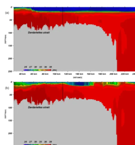
In the Dardanelles, the two-layered water mass and flow structure can be seen in Fig. 13. The simulated layered-structure in the Dardanelles is similar to those of Sannino et al. (2017, Fig. 7) under normal atmospheric conditions (Fig. 13a). The severe storm event on 22 November 2008 results in extensive mixing in the upper layer (Fig. 13b) where the salinity increases substantially. Furthermore, even the stratification is broken partially on the Sea of Marmara side of the strait.
south-Figure 11.Sea level difference (SLD) between Yalova and ¸Sile and daily averages of the meridional wind speed at B1 (see Fig. 1) between 2008 and 2011. The SLDs in the in situ observation (OBS) and the simulation (SIM) in metres are shown by the blue and red lines, respectively. The meridional wind speed is in orange in metres per second. The 4-year means, which are subtracted from the time series, are shown in the legend. A positive SLD means the sea level is higher in Yalova than in ¸Sile. A positive wind speed means the wind direction is northward. The grey circles mark the Orkoz events on 22 November 2008 and 21 August 2010 as suggested by the observations.
Figure 12. Cross-section of salinity in the Bosphorus strait on
(a) 15 November and(b) 22 November 2008 along the thalweg between 440 and 510 km. Contraction and the northern sill loca-tions are marked with green and cyan lines, respectively, as shown in Fig. 1.
ern Dardanelles, which are 39, 13.5, 22 and 13 m, respec-tively.
The net, annual mean upper layer and lower layer volume fluxes are given in Table 4, and the daily and monthly aver-ages are shown in Fig. 14. The estimations from Jarosz et al. (2011b, 2013) from direct measurements are also indicated. The mean net volume fluxes through the straits compare well with the observations between 2 September 2008 and 5 February 2009 for the Bosphorus, and 1 September 2008
Figure 13.Same as Fig. 12 but for the Dardanelles strait and its Sea of Marmara extension.
and 31 August 2009 for the southern Dardanelles. However, the variability in time is not as high as in the observations (Fig. 14). In the northern Dardanelles, there is a large dis-crepancy between the simulated net fluxes and the estimates from observations.
Figure 14.Daily upper layer (blue, UL), lower layer (red, LL) and net (grey, NET) volume fluxes through northern Bosphorus (NB), southern Bosphorus (SB), northern Dardanelles (ND) and southern Dardanelles (SD) in km3yr−1. Monthly and 6-year averages are overlaid with a darker tone of the same colour. The monthly aver-ages of volume fluxes computed by Jarosz et al. (2011b, 2013) are shown in green for the period of observations.
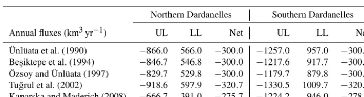
The historical estimates of the Dardanelles layer volume fluxes show much higher values than our simulation (Ta-ble 5). The changes found in the layer flux from one end of the strait to the other have been attributed to turbulent entrainment processes, which transport water and properties across the hypothesised layer interface (Ünlüata et al., 1990; Özsoy et al., 2001; Özsoy and Altıok, 2016). The larger dis-agreement of baroclinic volume fluxes compared to the net fluxes, and the lower estimations of the model layer fluxes, suggest that bottom friction parameterisation is too strong and possibly a problem in the vertical mixing submodel cho-sen.
The net volume transport in the model is approximately half of the historical estimations based on mass conserva-tion laws assuming a net water flux into the Black Sea of about 300 km3yr−1. Our choice to conserve the model vol-ume in a closed lateral boundary model by correcting the water flux every time step comes with the limitation of
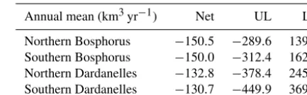
re-Table 4.Annual mean of net, upper layer and lower layer volume fluxes (km3yr−1) for the whole simulation period. A negative value indicates the flux is in the Black Sea – Aegean Sea direction.
Annual mean (km3yr−1) Net UL LL
Northern Bosphorus −150.5 −289.6 139.1 Southern Bosphorus −150.0 −312.4 162.4 Northern Dardanelles −132.8 −378.4 245.6 Southern Dardanelles −130.7 −449.9 369.2
ducing the transport along its way from the Black Sea to the Aegean Sea. The total water flux over the Sea of Marmara is
−17.1 km3yr−1(Fig. 3b) which is balanced by the difference between the southern Bosphorus and northern Dardanelles (Table 4). Due to the surface flux correction, the net outflow in the Dardanelles is decreased by about 10 % with respect to what entered the Bosphorus. However, such correction al-lowed us to obtain realistic salinity profiles with respect to other correction methods such as that used by Gürses et al. (2016).
Finally, the differences in transport between the transects at the two ends of each strait are 0.5 and 2.1 km3yr−1in the Bosphorus and Dardanelles, respectively. We attribute these differences partially again to the water flux correction at the surface. The rest is due to the numerical errors accumulating during the post-processing of the model outputs.
3.4 Dynamics and circulation in the Sea of Marmara Using the 6-year simulation, it is now possible to estimate the kinetic energy input by the wind in the Sea of Marmara.
The time series of monthly mean wind stress is shown in Fig. 15. It exhibits interannual differences with a mean of about 0.03 Nm−2and a maximum of around 0.05 Nm−2in August 2008. The monthly mean is highly variable and there is not a well-defined seasonal cycle between 2008 and 2013. The wind work normalised by the density and surface area is computed as
1 ρ0A
Z
A
τ·usdxdy, (3)
whereρ0is the surface density,τis the wind stress,usis the current velocity at the surface, andAis the surface area of the Sea of Marmara. The wind work is positively correlated with the wind stress. It is highest in 2011 and the maximum monthly mean wind work is 9.1×10⁻⁶m3s−3in the autumn of 2011.
Figure 15.Monthly time series of the wind work (m s ) and wind stress (Nm ) in the Sea of Marmara. The wind work normalised by the density and surface area of the Sea of Marmara is shown in grey in the right vertical axis. The wind stress is the black curve and its values are shown on the left vertical axis.
Table 5.Annual means of volume fluxes (km3yr−1) through the Dardanelles estimated by different studies. UL, LL and Net stand for upper layer, lower layer and net fluxes, respectively. A negative value indicates the volume flux is from the Sea of Marmara to the Aegean Sea.
Northern Dardanelles Southern Dardanelles
Annual fluxes (km3yr−1) UL LL Net UL LL Net
Ünlüata et al. (1990) −866.0 566.0 −300.0 −1257.0 957.0 −300.0 Be¸siktepe et al. (1994) −846.7 546.8 −300.0 −1217.6 917.7 −300.0 Özsoy and Ünlüata (1997) −829.7 529.8 −300.0 −1179.7 879.8 −300.0 Tu˘grul et al. (2002) −918.6 597.9 −320.7 −1330.5 1009.7 −320.8 Kanarska and Maderich (2008) −666.7 391.0 −275.7 −1224.2 946.0 −278.2
the Baltic Sea was computed to be 9.15×10⁻⁹m2s−3, which is comparable to the Sea of Marmara but is still lower.
The volume-mean kinetic energy in the Sea of Marmara normalised by the unit mass is calculated as 0.006 m2s−2 for 6 years. The daily mean kinetic energy time series re-veals that severe atmospheric events are able to energise the basin up to 0.03 m2s−2(not shown). The monthly volume-mean kinetic energy averages fluctuate between 0.005 and 0.01 m2s−2. It is higher in winter and early spring, whereas it is always below the mean in summer. The highest kinetic energy inputs are in October 2010, April 2011 and Novem-ber 2011. The kinetic energy is higher in the upper layer of the water column. The time mean of surface kinetic energy is about 0.03 m2s−2. Daily surface averages are capable of reaching 0.2 m2s−2. The monthly mean increases to approx-imately 0.05 m2s−2in November 2011.
In the Sea of Marmara, the buoyancy gain is mainly due to the Bosphorus inflow, and thus the latter competes with the wind work to change the kinetic energy of the basin, as explained by Cessi et al. (2014). However, at the surface, the kinetic energy shows that the Bosphorus surface jet energises the northeastern basin in addition to the wind (Fig. 16). The kinetic energy of the Bosphorus inflow is always greater than 0.075 m2s−2. In 2009, a kinetic energy maximum appears in the north of the Bozburun Peninsula where the Bosphorus jet arrives. In the western basin, the kinetic energy is generally less than 0.025 m2s−2. In 2011, the kinetic energy intensifies in the central north and exceeds 0.1 m2s−2. Almost all of the basin, except near the coastal areas, has a kinetic energy
higher than 0.025 m2s−2. Energy is mostly confined to the northeast of the central basin in 2013. The time mean for 2009–2013 reflects the characteristics of 2011 but with less amplitude.
The energetic Bosphorus jet generates a dipole vortic-ity field, which is anticyclonic in the west and cyclonic in the east (Fig. 17). Northern and western coasts are dom-inated by anticyclonic vorticity. Conversely, cyclonic vor-ticity dominates the southern coast. Positive and negative vorticity in the northern and southern coasts of the islands and peninsulas, respectively, are other common structures for all the years. The mean vorticity fields are consistent with upwelling-favourable conditions on the southern coasts of the Sea of Marmara. Primarily, a cyclonic gyre located at 28◦200N–40◦350E forms in the central basin after 2011, showing that the circulation changed sign between 2008 and 2011.
is-Figure 16.Annual mean of surface kinetic energy in the Sea of Marmara for(a)2009,(b)2011 and(c)2013.(d)The time mean of the 2009–2013 period. Units are in m2s−2as kinetic energy is normalised by the unit mass.
Figure 18.Annual mean of current velocity in the Sea of Marmara for(a)2009 at the surface,(b)2009 at 30 m,(c)2011 at the surface,
Figure 19.Schematic representation of the surface mean circulation in the Sea of Marmara for the 2009–2013 period. The thickness of curves shows the relative intensity of the associated current.
lands in the southwestern Sea of Marmara and eventually exiting from the Dardanelles. This circulation pattern in the western Sea of Marmara is persistent throughout the simu-lation but with different intensities. This type of circusimu-lation structure has been reported in other studies (Chiggiato et al., 2012; Be¸siktepe et al., 1994). In 2011 (Fig. 18c), the circu-lation in the middle of the Sea of Marmara evolves into a single cyclonic structure. The shift in the circulation can be explained by the shift of the wind stress maximum towards the north (Fig. 2). Sannino et al. (2017) demonstrates a sim-ilar cyclonic pattern in the central Sea of Marmara due to the potential vorticity input by the Bosphorus. However, in our case, the main driver of the cyclone should be the wind, as the volume transport through the Bosphorus is much lower than that of Sannino et al. (2017) case. Thus, in certain condi-tions, both the wind and the Bosphorus can induce a cyclonic circulation in the Sea of Marmara. The cyclonic surface cir-culation dominates the mean between 2009–2013. The mean surface circulation in the sea can be sketched as in Fig. 19.
Below the pycnocline at 30 m, two main structures can be identified. An anticyclonic formation appears in the cen-tral basin intensifying in 2013. On the Dardanelles side, a flow enters the Sea of Marmara and partially heads south-east. Another structure recirculates after reaching Marmara Island and joins the southwestward flow exiting the Sea of Marmara. In 2011, a meander heading west is formed in the northern basin. This feature is not present in other years and results from the deepening of the upper layer (not shown) due to stronger wind stress.
The mean circulation of the Sea of Marmara, schemati-cally shown in Fig. 19, is dominated by the Bosphorus jet and the Marmara jet meandering cyclonically. The mid-Marmara jet is divided into three before reaching mid-Marmara Island, and one branch heads to the northwest and the other two reach the Dardanelles after circulating around the island. Finally, weak currents move in an east–west direction on the southern coast of the basin.
4 Summary and discussion
We present a 6-year simulation of the Turkish Straits System, with a highly resolved unstructured mesh model of the TSS using realistic atmospheric forcing to identify the circulation structure and the interplay between the atmospheric forcing and the Bosphorus input. The results demonstrate that a re-alistic representation of the pycnocline from the two straits to the Sea of Marmara is possible. The model is capable of reproducing the historically reported water mass structure of the Sea of Marmara. Model errors peak at the halocline and thermocline depths, where small changes in the interface depth induce greater error.
The strait volume transport has been compared with the observations. The net volume transport in the Bosphorus agrees with the estimates based on the observations. The model solution departs from the observations in the northern Dardanelles, but closer agreement is found elsewhere. The baroclinic transport shows larger discrepancies between the observations and the model, possibly because of uncertain-ties in the bottom boundary layer dissipation mechanisms and turbulence parameterisation. The model is capable of simulating blocking events in the straits during severe storm passages, to the extent that such storms are present in the at-mospheric dataset, as shown for the 22 November 2008 case. The circulation in the Sea of Marmara shows two patterns in the interannual timescales. The first is dominated by the buoyant plume of the Bosphorus to the south around an an-ticyclonic circulation structure in the eastern and northern parts of the basin. This type of circulation has been observed and modelled by several earlier studies (Be¸siktepe et al., 1994; Chiggiato et al., 2012; Sannino et al., 2017). The other circulation structure includes a cyclone in the central basin because of intensifying and expanding wind stress over the Sea of Marmara. Small-scale vortices are also formed in var-ious parts of the basin and a larger one appears in the north-west after 2011. The cyclonic gyre in the central Sea of Mar-mara is shown numerically only by Sannino et al. (2017), in the case of extreme net volume flux through the Bosphorus. However, here, we show that the wind can produce the cy-clonic circulation in addition to the Bosphorus jet.
The long-term simulation with atmospheric forcing made it possible to evaluate the wind energy input and compute the kinetic energy in the Sea of Marmara. The wind work in the Sea of Marmara is shown to be even higher than the Baltic Sea. The high energy input from the wind significantly increases the kinetic energy in the Sea of Marmara. During severe storms, kinetic energy can increase by 10 times the time-averaged value. The annual mean of kinetic energy in the regions under the influence of the wind forcing can also exceed that from the Bosphorus jet, depending on the wind stress structure.
atmospheric forcing used in the simulation. Within the rel-atively small domain of the TSS, an improved representa-tion of the atmospheric forcing, particularly during the se-vere storms frequenting the region in winter, appears to be essential for improving its skill.
do˘gdu et al. (2018), should also be considered for a better state estimate.
Appendix A: Model equations
FESOM solves the standard set of hydrostatic primitive equa-tions with the Boussinesq approximation (Wang et al., 2008).
The momentum equations are ∂tu+v· ∇3u+fkˆ×u= −
1 ρ0
∇p −g∇η− ∇Ah∇(∇2u)
+∂zAv∂zu, (A1)
whereu=(u, v)andv=(u, v, w)are 2-D and 3-D veloc-ities, respectively, in the spherical coordinate system, ρ0 is the mean density,gis the gravitational acceleration,ηis the sea surface elevation, f is the Coriolis parameter, andkˆ is the vertical unit vector.∇ and∇3stand for 2-D and 3-D gra-dients or divergence operators, respectively. The horizontal and vertical viscosities are denoted byAh andAv.p is the hydrostatic pressure obtained integrating the hydrostatic re-lation (Eq. A3) fromz=η. Atmospheric pressure is not con-sidered in order to not excite basin modes in a closed lateral boundary model.
The Laplacian viscosity is known to be generally too damping and strongly reduces the eddy variances of all fields compared to observations when the model is run at eddy resolving resolutions (Wang et al., 2008). Therefore, bihar-monic viscosity is used in the momentum equations. Here, Ahis scaled by the cube of the element size with a reference valueAh0of 2.7×10¹³m4s−1(Table A1), which is set for the reference resolution of 1◦.
The continuity equation is used to diagnose the vertical velocityw:
∂zw= −∇ ·u, (A2)
and the hydrostatic equation is
∂zp= −gρ, (A3)
whereρis the deviation from the mean densityρ0. Tracer Eqs. (A4) and (A5),
∂tT +v· ∇3T− ∇ ·Kh∇T−∂zKv∂zT =0 (A4)
∂tS+v· ∇3S− ∇ ·Kh∇S−∂zKv∂zS=0, (A5)
are solved for the potential temperature, T, and salinity,S, whereKh andKv are the horizontal and vertical eddy dif-fusivities, respectively. Laplacian diffusivity is used for the tracer equations.Khis again scaled asAhbut by the element size with a reference value of 2.0×10³m2s−1. These values are set following the convergence study of Wallcraft et al. (2005).
The Pacanowski and Philander (1981) (PP) parameterisa-tion scheme is used for vertical mixing, with a background vertical viscosity of 10−5m2s−1 for momentum and diffu-sivity of 10−6m2s−1for tracers. The maximum value is set to 0.005 m2s−1.
The density anomalyρis computed by the full equation of state (Eq. A6).
ρ=ρ(T , S, p) (A6)
The surface and bottom momentum boundary conditions are, respectively,
Av∂zu=τ (A7)
Av∂zu+Ah∇H· ∇u=Cdu|u|, (A8) whereτ andCdare the wind stress and the surface drag co-efficient, respectively.
The surface kinematic boundary condition is
w=∂tη+u· ∇η+(E−P−R)+Wcorr, (A9) whereE(m s−1) andP (m s−1) are evaporation and precipi-tation, respectively.R(km3yr−1) is runoff (see Table 1). It is converted to m3s−1and normalised by the area of the buffer zone in the Black Sea (see Fig. 1) before entering to the equa-tion. Finally, Wcorr is a correction applied to conserve the volume of the model, as described later.
The sea surface height equation can now be derived from Eqs. (A2) and (A9) as
∂tη+ ∇ · z=η Z
z=−H
udz= −(E−P−R)−Wcorr. (A10)
The upper limit of integration in Eq. (A10) is set toηin this version of FESOM and is different from Wang et al. (2008) to provide a non-linear free surface solution.
The bottom boundary conditions for the temperature and salinity are
(∇T , ∂zT )·n3=0 (A11)
(∇S, ∂zS)·n3=0, (A12)
wheren3is the 3-D unit vector normal to the respective sur-face.
The surface boundary condition for temperature is Kv∂zT
z=η=
Q ρ0Cp
, (A13)
whereCp=4000 J kg−1K−1andQ(W m−2) is the surface
net heat flux into the ocean.
In global applications, surface salinity is generally relaxed to a climatology to prevent a drift. In our regional application, the water flux term in the boundary condition (Eq. A14) is applied over the whole domain, whereas the relaxation term is prescribed only in the Black Sea buffer zone.
Kv∂zS
RB Black Sea runoff Table 1
S0 Sea surface salinity psu
S∗ Salinity relaxed in the Black Sea buffer zone Table 1 psu
γ Salinity relaxation coefficient 5.79×10⁻⁶ m s−1
Wcorr Water flux correction m s−1
Scorr Salinity flux correction psu m s−1
Ah0 Horizontal eddy viscosity reference value 2.7×10¹³ m4s−1
Kh0 Horizontal eddy diffusivity reference value 2.0×10³ m2s−1
Av0 Vertical background viscosity 1.0×10⁻⁵ m2s−1
Kv0 Vertical background diffusivity 1.0×10⁻⁶ m2s−1
Appendix B: Salt conservation properties
As our model domain is closed, we need to enforce salt con-servation. Volume salinity conservation requires the time rate of the change in the volume salinity term in Eq. (B1) to be zero. A balance must be satisfied between the two integrals.
∂ ∂t
Z Z Z
V
SdV = Z Z
AD
(Kv∂zS
z=η)dAD=0 (B1)
In FESOM, this balance is achieved by applying a cor-rection for each term separately. The amount of water flux by evaporation, precipitation and runoff is integrated over the surface with every time step (Eq. B2). After normalising by the domain area as in Eq. (B3), the surplus or deficit is added to or subtracted from the total water flux equally from each node of the mesh with theWcorrterms in Eqs. (A9) and (A10).
1(E−P−R)= Z
x,y
(E−P−R)dxdy (B2)
Wcorr=
1E−P−R
AD
(B3)
The salinity flux is corrected in a similar manner for the boundary condition:
1S= Z
x,y
(S0(E−P−R)+γ (S∗−S0))dxdy (B4)
Scorr= 1S AD
. (B5)
Author contributions. ÖG and AA implemented the model in the Turkish Straits System. AA, NP and EÖ designed the experiment. AA analysed the results. AA, NP, EÖ and GD contributed to the interpretation of the results and writing the paper. AK contributed to the interpretation of the results.
Competing interests. The authors declare that they have no conflict of interest.
Acknowledgements. The simulations in this study are performed in the CMCC/ATHENA cluster. The work is a part of the PhD study of Ali Aydo˘gdu and funded by Ca’ Foscari University of Venice and CMCC. The preparation of the manuscript continued under the funding of the REDDA project of the Norwegian Research Council under contract 250711 during his post-doctoral research. NCAR is sponsored by the US National Science Foundation. The authors thank Georg Umgiesser, two anonymous referees and the editor for their careful assessment of the manuscript which helped us to improve it substantially.
Edited by: Markus Meier
Reviewed by: Georg Umgiesser and two anonymous referees
References
Alpar, B., Do˘gan, E., Yüce, H., and Altıok, H.: Sea level changes along the Turkish coasts of the Black Sea, the Aegean Sea and the Eastern Mediterranean, Mediterr. Mar. Sci., 1, 141–156, 2000. Altıok, H., Sur, H. ˙I., and Yüce, H.: Variation of the cold
intermedi-ate wintermedi-ater in the Black Sea exit of the Strait of Istanbul (Bospho-rus) and its transfer through the strait, Oceanologia, 54, 233–254, 2012.
Aydogdu, A., Hoar, T. J., Vukicevic, T., Anderson, J. L., Pinardi, N., Karspeck, A., Hendricks, J., Collins, N., Macchia, F., and Özsoy, E.: OSSE for a sustainable marine observing network in the Sea of Marmara, Nonlin. Processes Geophys., 25, 537–551, https://doi.org/10.5194/npg-25-537-2018, 2018.
Be¸siktepe, ¸S. T., Sur, H. I., Özsoy, E., Latif, M. A., O˘guz, T., and Ünlüata, Ü.: The circulation and hydrography of the Marmara Sea, Prog. Oceanogr., 34, 285–334, 1994.
Bogdanova, C.: Seasonal fluctuations in the inflow and distribution of the Mediterranean waters in the Black Sea, in: Basic Features of the Geological Structure, of the Hydrologic Regime and Bi-ology of the Mediterranean Sea, Academy of Sciences, USSR, Moskow., 131–139, english translation 1969 Institute of Modem Languages, Washington DC, 1969.
Book, J. W., Jarosz, E., Chiggiato, J., and Be¸siktepe, ¸S.: The oceanic response of the Turkish Straits System to an extreme drop in at-mospheric pressure, J. Geophys. Res.-Oceans, 119, 3629–3644, https://doi.org/10.1002/2013JC009480, 2014.
Büyükay, M.: The surface and internal oscillations in the Bospho-rus, related to meteorological forces, Master’s thesis, Institute of Marine Sciences, Middle East Technical University, Erdemli, Içel, Turkey, 1989.
Cessi, P., Pinardi, N., and Lyubartsev, V.: Energetics of Semien-closed Basins with Two-Layer Flows at the Strait, J.
Phys. Oceanogr., 44, 967–979, https://doi.org/10.1175/JPO-D-13-0129.1, 2014.
Chiggiato, J., Jarosz, E., Book, J. W., Dykes, J., Torrisi, L., Poulain, P. M., Gerin, R., Horstmann, J., and Be¸siktepe, ¸S.: Dynamics of the circulation in the Sea of Marmara: Numer-ical modeling experiments and observations from the Turk-ish straits system experiment, Ocean Dynam., 62, 139–159, https://doi.org/10.1007/s10236-011-0485-5, 2012.
Courant, R., Friedrichs, K., and Lewy, H.: On the partial difference equations of mathematical physics, IBM J. Res. Dev., 11, 215– 234, 1967.
Danilov, S., Kivman, G., and Schröter, J.: A finite-element ocean model: principles and evaluation, Ocean Model., 6, 125–150, 2004.
Demyshev, S., Dovgaya, S., and Ivanov, V.: Numerical modeling of the influence of exchange through the Bosporus and Dardanelles Straits on the hydrophysical fields of the Marmara Sea, Izvestiya, Atmospheric and Oceanic Physics, 48, 418–426, 2012.
Dorrell, R., Peakall, J., Sumner, E., Parsons, D., Darby, S., Wynn, R., Özsoy, E., and Tezcan, D.: Flow dynamics and mixing pro-cesses in hydraulic jump arrays: Implications for channel-lobe transition zones, Mar. Geol., 381, 181–193, 2016.
Falina, A., Sarafanov, A., Özsoy, E., and Utku Turunço˘glu, U.: Observed basin-wide propagation of Mediterranean water in the Black Sea, J. Geophys. Res.-Oceans, 122, 3141–3151, https://doi.org/10.1002/2017JC012729, 2017.
Federico, I., Pinardi, N., Coppini, G., Oddo, P., Lecci, R., and Mossa, M.: Coastal ocean forecasting with an un-structured grid model in the southern Adriatic and north-ern Ionian seas, Nat. Hazards Earth Syst. Sci., 17, 45–59, https://doi.org/10.5194/nhess-17-45-2017, 2017.
Ferrarin, C., Bellafiore, D., Sannino, G., Bajo, M., and Umgiesser, G.: Tidal dynamics in the inter-connected Mediterranean, Mar-mara, Black and Azov seas, Prog. Oceanogr., 161, 102–115, 2018.
Ford, R., Pain, C., Piggott, M., Goddard, A., De Oliveira, C., and Umpleby, A.: A nonhydrostatic finite-element model for three-dimensional stratified oceanic flows. Part I: model formulation, Mon. Weather Rev., 132, 2816–2831, 2004.
Gent, P. R., Bryan, F. O., Danabasoglu, G., Doney, S. C., Holland, W. R., Large, W. G., and McWilliams, J. C.: The NCAR climate system model global ocean component, J. Climate, 11, 1287– 1306, 1998.
Gregg, M. C. and Özsoy, E.: Flow, water mass changes, and hydraulics in the Bosphorus, J. Geophys. Res., 107, 3016, https://doi.org/10.1029/2000JC000485, 2002.
Gunnerson, C. G. and Ozturgut, E.: The Bosporus, The Black Sea– geology, chemistry and biology, AAPG Bull, 20, 99–114, 1974. Gürses, Ö., Aydo˘gdu, A., Pinardi, N., and Özsoy, E.: A finite
ele-ment modeling study of the Turkish Straits System, in: The Sea of Marmara – Marine Biodiversity, Fisheries, Conservations and Governance, edited by: Özsoy E., Çaˇgatay, M. N., Balkis, N., and Öztürk, B., TUDAV Publication, 169–184, 2016.
Hüsrevo˘glu, S.: Modeling Of The Dardanelles Strait Lower-layer Flow Into The Marmara Sea, Master’s thesis, Institute of Marine Sciences, METU, 1998.
Jarosz, E., Teague, W. J., Book, J. W., and Be¸siktepe, ¸S.: Observed volume fluxes and mixing in the Dard-anelles Strait, J. Geophys. Res.-Oceans, 118, 5007–5021, https://doi.org/10.1002/jgrc.20396, 2013.
Johns, B. and O˘guz, T.: The modelling of the flow of water through the Bosphorus, Dynam. Atmos. Oceans, 14, 229–258, 1989. Jordà, G., Von Schuckmann, K., Josey, S. A., Caniaux, G.,
García-Lafuente, J., Sammartino, S., Özsoy, E., Polcher, J., Notarste-fano, G., Poulain, P.-M., Adloff, F., Salat, J., Naranjo, C., Schroeder, K., Chiggiato, J., Sannino, G., and Macías, D.: The Mediterranean Sea heat and mass budgets: estimates, un-certainties and perspectives, Prog. Oceanogr., 156, 174–208, https://doi.org/10.1016/j.pocean.2017.07.001, 2017.
Kanarska, Y. and Maderich, V.: Modelling of seasonal exchange flows through the Dardanelles Strait, Estuar. Coast. Shelf S., 79, 449–458, 2008.
Kara, A. B., Wallcraft, A. J., Hurlburt, H. E., and Stanev, E.: Air– sea fluxes and river discharges in the Black Sea with a focus on the Danube and Bosphorus, J. Marine Syst., 74, 74–95, 2008. Maderich, V. and Konstantinov, S.: Seasonal dynamics of the
sys-tem sea-strait: Black Sea–Bosphorus case study, Estuar. Coast. Shelf S., 55, 183–196, 2002.
Maderich, V., Ilyin, Y., and Lemeshko, E.: Seasonal and interannual variability of the water exchange in the Turkish Straits System estimated by modelling, Mediterr. Mar. Sci., 16, 444–459, 2015. Marshall, J., Adcroft, A., Hill, C., Perelman, L., and Heisey, C.: A finite-volume, incompressible Navier Stokes model for studies of the ocean on parallel computers, J. Geophys. Res.-Oceans, 102, 5753–5766, https://doi.org/10.1029/96JC02775, 1997.
McDougall, T. J.: Neutral surfaces, J. Phys. Oceanogr., 17, 1950– 1964, 1987.
Moller, L.: Alfred Merz Hydrographiche unter Suchungen in Bosphorus and Dardanalten, Veroff. Insr. Meeresk, Berlin Uni., Neue Folge A, 18, 1928.
Oddo, P., Adani, M., Pinardi, N., Fratianni, C., Tonani, M., and Pet-tenuzzo, D.: A nested Atlantic-Mediterranean Sea general circu-lation model for operational forecasting, Ocean Sci., 5, 461–473, https://doi.org/10.5194/os-5-461-2009, 2009.
O˘guz, T. and Sur, H.: A 2-layer model of water exchange through the Dardanelles strait, Oceanol. Acta, 12, 23–31, 1989.
O˘guz, T., Özsoy, E., Latif, M. A., Sur, H. I., and Ünlüata, Ü.: Mod-eling of hydraulically controlled exchange flow in the Bosphorus Strait, J. Phys. Oceanogr., 20, 945–965, 1990.
Özsoy, E. and Altıok, H.: A review of water fluxes across the Turk-ish Straits System, in: The Sea of Marmara – Marine Biodiver-sity, Fisheries, Conservations and Governance, edited by: Özsoy, E., Çaˇgatay, M. N., Balkis, N., and Öztürk, B., TUDAV Publica-tion, 42–61, 2016.
Strait: Exchange fluxes, currents and sea-level changes, NATO Science Series 2, Environmental Security, 47, 1–28, 1998. Özsoy, E., Di Iorio, D., Gregg, M. C., and Backhaus, J. O.:
Mix-ing in the Bosphorus Strait and the Black Sea continental shelf: observations and a model of the dense water outflow, J. Marine Syst., 31, 99–135, 2001.
Öztürk, M., Ayat, B., Aydo˘gan, B., and Yüksel, Y.: 3D Numeri-cal Modeling of Stratified Flows: Case Study of the Bosphorus Strait, Journal of Waterway, Port, Coastal, and Ocean Engineer-ing, 138, 406–419, https://doi.org/10.1061/(ASCE)WW.1943-5460.0000132, 2012.
Pacanowski, R. and Philander, S.: Parameterization of vertical mix-ing in numerical models of tropical oceans, J. Phys. Oceanogr., 11, 1443–1451, 1981.
Peneva, E., Stanev, E., Belokopytov, V., and Le Traon, P.-Y.: Wa-ter transport in the Bosphorus Straits estimated from hydro-meteorological and altimeter data: seasonal to decadal variabil-ity, J. Marine Syst., 31, 21–33, 2001.
Sannino, G., Sözer, A., and Özsoy, E.: A high-resolution modelling study of the Turkish Straits System, Ocean Dynam., 67, 397–432, https://doi.org/10.1007/s10236-017-1039-2, 2017.
Schroeder, K., Garcìa-Lafuente, J., Josey, S. A., Artale, V., Buon-giorno Nardelli, B., Carrillo, A., Gaˇci´c, M., Gasparini, G. P., Herrmann, M., Lionello, P., Ludwig, W., Millot, C., Özsoy, E., Pisacane, G., Sánchez-Garrido, J. C., Sannino, G., Santoleri, R., Somot, S., Struglia, M., Stanev, E., Taupier-Letage, I., Tsimplis, M. N., Vargas-Yáñez, M., Zervakis, V., and Zodiatis, G.: Circula-tion of the Mediterranean Sea and its variability, in: The Climate of the Mediterranean Region – From the past to the future, edited by: Lionello, P., Elsevier, p. 592, https://doi.org/10.1016/B978-0-12-416042-2.00003-3, 2012.
Sözer, A. and Özsoy, E.: Modeling of the Bosphorus exchange flow dynamics, Ocean Dynam., 67, 1–23, https://doi.org/10.1007/s10236-016-1026-z, 2017a.
Sözer, A. and Özsoy, E.: Water Exchange through Canal ˙Istanbul and Bosphorus Strait, Mediterr. Mar. Sci., 18, 77–86, 2017b. Stanev, E. V., Grashorn, S., and Zhang, Y. J.: Cascading ocean
basins: numerical simulations of the circulation and interbasin exchange in the Azov-Black-Marmara-Mediterranean Seas sys-tem, Ocean Dynam., 67, 1–23, 2017.
Stashchuk, N. and Hutter, K.: Modelling of water exchange through the Strait of the Dardanelles, Cont. Shelf Res., 21, 1361–1382, 2001.
Storto, A., Ciliberti, S., Peneva, E., and Macchia, F.: Quality In-formation Document for Black Sea Physical Reanalysis product, Tech. rep., Copernicus Marine Environment Monitoring Service, 2016.
2011, in: The Sea of Marmara – Marine Biodiversity, Fisheries, Conservations and Governance, edited by: Özsoy, E., Çaˇgatay, M. N., Balkis, N., and Öztürk, B., TUDAV Publication, 2016. Tu˘grul, S., Be¸siktepe, T., and Saliho˘glu, I.: Nutrient exchange fluxes
between the Aegean and Black Seas through the Marmara Sea, Mediterr. Mar. Sci., 3, 33–42, 2002.
Umgiesser, G., Canu, D. M., Cucco, A., and Solidoro, C.: A finite element model for the Venice Lagoon. Development, set up, cal-ibration and validation, J. Marine Syst., 51, 123–145, 2004. Ünlüata, Ü., O˘guz, T., Latif, M., and Özsoy, E.: On the physical
oceanography of the Turkish Straits, in: The physical oceanogra-phy of sea straits, Springer, 25–60, 1990.
Wallcraft, A. J., Kara, A. B., and Hurlburt, H. E.: Con-vergence of Laplacian diffusion versus resolution of an ocean model, Geophys. Res. Lett., 32, l07604, https://doi.org/10.1029/2005GL022514, 2005.
Wang, Q., Danilov, S., and Schröter, J.: Finite element ocean circulation model based on triangular prismatic ele-ments, with application in studying the effect of topogra-phy representation, J. Geotopogra-phys. Res.-Oceans, 113, C05015, https://doi.org/10.1029/2007JC004482, 2008.
White, L., Legat, V., and Deleersnijder, E.: Tracer conservation for three-dimensional, finite-element, free-surface, ocean modeling on moving prismatic meshes, Mon. Weather Rev., 136, 420–442, 2008.
Xie, P. and Arkin, P. A.: Global precipitation: A 17-year monthly analysis based on gauge observations, satellite estimates, and nu-merical model outputs, B. Am. Meteorol. Soc., 78, 2539–2558, 1997.