www.atmos-meas-tech.net/8/267/2015/ doi:10.5194/amt-8-267-2015
© Author(s) 2015. CC Attribution 3.0 License.
Development and validation of inexpensive, automated, dynamic
flux chambers
B. B. Almand-Hunter1, J. T. Walker2, N. P. Masson1, L. Hafford1, and M. P. Hannigan1
1Mechanical Engineering Department, University of Colorado, 427 UCB, Boulder, CO, 80303, USA
2Air Pollution Prevention and Control Division, National Risk Management Research Laboratory, US Environmental
Protection Agency, E305-2, MD-63, Research Triangle Park, NC 27711, USA Correspondence to: B. B. Almand-Hunter ([email protected])
Received: 15 May 2014 – Published in Atmos. Meas. Tech. Discuss.: 10 July 2014 Revised: 29 October 2014 – Accepted: 19 November 2014 – Published: 13 January 2015
Abstract. We developed and validated an automated, inex-pensive, and continuous multiple-species gas-flux monitor-ing system that can provide data for a variety of relevant atmospheric pollutants, including O3, CO2, and NOx.
Val-idation consisted of conducting concurrent gas-phase dry-deposition experiments, using both dynamic flux chambers and an eddy-covariance system, in a grassy clearing in the Duke Forest (Chapel Hill, NC). Experiments were carried out in June and September under a variety of meteorological con-ditions. Ozone-deposition measurements from the two meth-ods matched very well (4–10 % difference in mean flux rate) when the leaf-area index (LAI) inside the chambers was rep-resentative of the average LAI in the field. The dynamic flux chambers can be considered an accurate measurement sys-tem under these conditions.
1 Introduction
Deposition of pollutants – including ozone, nitrogen, and acidic compounds (SOx, NOy) – places environmental
stress on sensitive vegetated landscapes and aquatic ecosys-tems (Driscoll et al., 2001; Williams and Tonnessen, 2000; Fangmeier et al., 1994). Examples of this stress include in-creased susceptibility to injury (DeHayes et al., 1999) and decreased growth for sensitive plant species, decreased wa-ter quality, toxicity to freshwawa-ter organisms, eutrophication, change in greenhouse emissions from soil (Fenn et al., 1998), reduction in biodiversity, and interference with a plant’s up-take of other important cations, such as potassium (Fang-meier et al., 1994). These negative effects can be
particu-larly pronounced at high altitudes, where buffering capacities can be below average (Fenn et al., 1998; Williams and Ton-nessen, 2000; Benedict et al., 2013). There has been debate over whether ozone damage to vegetation is best quantified and regulated using ambient concentrations or atmospheric fluxes (Musselman et al., 2006). While the use of ambient concentrations is certainly much simpler, fluxes have more physical meaning.
Dry deposition, which is the process by which pollutants are transported from the atmosphere to the earth’s surface without precipitation (Seinfeld and Pandis, 2006), is an im-portant component of atmospheric deposition. This process is estimated to account for up to 50 % of total atmospheric deposition in the United States (EPA, 2010; Wesely and Hicks, 2000). Despite this sizable contribution to total at-mospheric deposition, there is a shortage of direct ments of dry deposition in the US. Because of this measure-ment shortage, improving deposition models is crucial. Ad-ditionally, understanding deposition and emission rates is an important piece of estimating atmospheric concentrations in the planetary boundary layer for climate and weather mod-els. Efforts to improve deposition models are ongoing (Say-lor et al., 2014; Zhang et al., 2003; Brook et al., 1999; Pleim et al., 2013), and models estimate flux well under some con-ditions, but fluxes determined by different models and obser-vations can vary by a factor of 2 to 3 (Schwede et al., 2011; Wu et al., 2011; Flechard et al., 2011). Direct dry-deposition measurements are needed to improve and validate models for a variety of ecosystems and environmental conditions.
prohibitively expensive and complex. This results in signif-icant uncertainty in deposition loads, specifically regarding transfer ratios (the relationship between ambient concentra-tions and total deposition). Given the large spatiotemporal variability in air–surface exchange rates of reactive com-pounds, there is a need for low-cost, easily deployable sys-tems to measure dry deposition directly. These measurement devices should be automated and remotely controlled, so that they can be deployed for extended periods of time without excessive maintenance.
Currently, the most accurate direct method for measuring atmospheric fluxes is eddy covariance (Seinfeld and Pan-dis, 2006; Turnipseed et al., 2009). Eddy covariance con-sists of taking high-speed measurements of concentration and three-dimensional wind velocity. The flux is computed from the covariance between the fluctuating components of wind velocity and concentration (Turnipseed et al., 2009). This method is the most mathematically robust and accurate way to acquire dry-deposition measurements, but it is expen-sive and technically difficult compared with indirect mea-surement methods (Baldocchi et al., 1988).
Another method for measuring flux, which is used more frequently to measure emissions than it is to measure de-position, is the flux chamber. Advantages of flux chambers over eddy covariance include reduced cost, the ability to de-termine spatial variability in deposition, the ability to take measurements in areas with complex topography and areas with non-uniform vegetation (eddy covariance typically re-quires an area of uniform vegetation that is≥100 m2), mo-bility, and the potential to be used with inexpensive sensors (Horst and Weil, 1994). The main drawback of using cham-bers for flux measurements is that they alter the environment in which they are placed. Static chambers, which are com-monly used to measure emissions, significantly affect envi-ronmental conditions (Pape et al., 2009).
Dynamic flux chambers minimize the alteration of envi-ronmental conditions by constantly pumping ambient air into the chamber. Table 1 lists previous flux-chamber measure-ments of NO, NO2, CO2, and O3. One type of flux chamber
listed in Table 1 is the leaf-scale dynamic chamber, which is used to measure fluxes to and from individual leaves and branches (Breuninger et al., 2012, 2013; Geßler et al., 2000; Sparks et al., 2001; Altimir et al., 2002). While leaf-scale de-position measurements are important for understanding plant dynamics, they can be difficult to translate to the canopy scale and do not directly represent ecosystem-level flux.
Another type of chamber listed in Table 1 is the dynamic soil-flux chamber (Remde et al., 1993; Norman et al., 1997). A significant portion of the chambers listed did not have open tops, and the soil or vegetation in the chamber was only ex-posed to ambient conditions via air pumped into the chamber. These chambers, which are not normally open to the ambi-ent environmambi-ent, have significant drawbacks. They all block a fraction of incoming solar radiation, and in order to
main-tain ambient conditions they have to be moved frequently, which makes long-term or remote deployments difficult.
Several research groups have addressed these issues by de-veloping chambers with lids that open and close automati-cally (Meixner et al., 1997; Pape et al., 2009; Kitzler et al., 2006). These automatic chambers operate in a normally open mode, with lids that close for just a few minutes per hour. Provided that the chambers are made out of highly transpar-ent materials, so sunlight can reach the vegetation inside, the environmental conditions in the chamber remain very close to ambient (Pape et al., 2009).
While many chamber measurements have been made (Ta-ble 1), very few of these studies compare O3fluxes measured
by chambers to measurements acquired via micrometeoro-logical techniques. Several groups have compared chamber measurements of NO fluxes from soils to gradient measure-ments (Parrish et al., 1987; Stella et al., 2012). Norman et al. (1997) compared several types of static and dynamic cham-bers with each other and eddy correlation for measuring CO2
fluxes in forest soils, but only two data points for eddy corre-lation were available for comparison, each representing one day. Li et al. (1999) compared chamber measurements of NO fluxes from agricultural soils with eddy-correlation measure-ments and found that the fluxes measured by the chambers were higher than the eddy-correlation measurements but fol-lowed a similar diurnal trend. Pape et al. (2009) compared an automatic, dynamic flux chamber with an eddy-covariance system at a grassland site and demonstrated good agreement for CO2 deposition. Due to the fact that these comparison
studies are limited in number, and sometimes did not yield good agreement between methods, further comparisons of flux chambers and micrometeorological methods are war-ranted.
Our research effort expands on this validation-based flux-chamber development through the creation of an automated, inexpensive, and continuous multiple-species gas-flux mon-itoring system, which can provide data for a variety of rel-evant atmospheric pollutants, including O3, CO2, and NOx.
The chambers have automatic lids, which keep the environ-ment in the chambers close to ambient, and eliminate the need to regularly remove them from sampling plots. This project is unique because our chambers not only build on the limited chamber-validation literature, but also utilize an inexpensive design (<USD 2000 each). The chambers are equipped with inexpensive metal-oxide O3 and NO2
sen-sors, which cost between USD 10 and 100, and our ultimate goal is to obtain fluxes using these inexpensive sensors. The first step toward reaching that goal is to use data from estab-lished O3, CO2, and NOx monitors to validate the dynamic
flux-chamber measurements, which enables us to isolate the uncertainty related to the use of inexpensive sensors from chamber performance. We present preliminary results, com-paring chamber fluxes to eddy-covariance fluxes for O3and
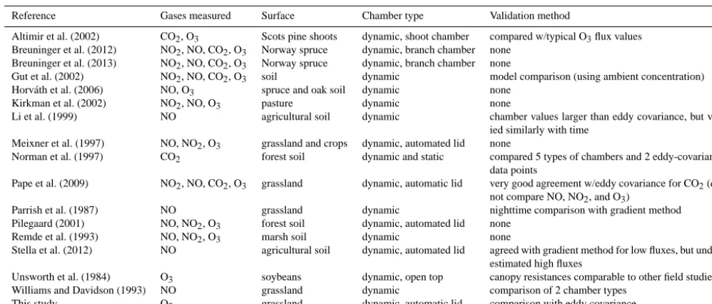
Table 1. Summary of selected chamber measurements of NO2, NO, O3, and CO2.
Reference Gases measured Surface Chamber type Validation method
Altimir et al. (2002) CO2, O3 Scots pine shoots dynamic, shoot chamber compared w/typical O3flux values
Breuninger et al. (2012) NO2, NO, CO2, O3 Norway spruce dynamic, branch chamber none
Breuninger et al. (2013) NO2, NO, CO2, O3 Norway spruce dynamic, branch chamber none
Gut et al. (2002) NO2, NO, CO2, O3 soil dynamic model comparison (using ambient concentration)
Horváth et al. (2006) NO, O3 spruce and oak soil dynamic none
Kirkman et al. (2002) NO2, NO, O3 pasture dynamic none
Li et al. (1999) NO agricultural soil dynamic chamber values larger than eddy covariance, but var-ied similarly with time
Meixner et al. (1997) NO, NO2, O3 grassland and crops dynamic, automated lid none
Norman et al. (1997) CO2 forest soil dynamic and static compared 5 types of chambers and 2 eddy-covariance
data points
Pape et al. (2009) NO2, NO, CO2, O3 grassland dynamic, automatic lid very good agreement w/eddy covariance for CO2(did
not compare NO, NO2, and O3)
Parrish et al. (1987) NO grassland dynamic nighttime comparison with gradient method
Pilegaard (2001) NO, NO2, O3 forest soil dynamic, automated lid none
Remde et al. (1993) NO, NO2, O3 marsh soil dynamic none
Stella et al. (2012) NO agricultural soil dynamic, automated lid agreed with gradient method for low fluxes, but under-estimated high fluxes
Unsworth et al. (1984) O3 soybeans dynamic, open top canopy resistances comparable to other field studies
Williams and Davidson (1993) NO grassland dynamic comparison of 2 chamber types
This study O3 grassland dynamic, automatic lid comparison with eddy covariance
2 Methods 2.1 Overview
We conducted gas-phase dry-deposition experiments in a grassy clearing in the Blackwood Division of Duke For-est in Orange County, North Carolina, USA (35.97◦N, 79.09◦W). The field is 480 m×305 m, and the vegetation is primarily tall fescue (Festuca arundinacea Shreb.), which is a common C3 grass in the southeastern United States. Less-prominent vegetation includes C3 and C4 grasses, herbs, and forbs, which are present in smaller amounts (Fluxnet, 2013). We used five pairs of acrylic-glass flux chambers to mea-sure dry deposition of NOx, O3, and CO2 to the
grass-land vegetation. Experiments were carried out in June and September, under a variety of meteorological conditions. We compared the chamber results with eddy-covariance mea-surements, which were conducted by the EPA at the same site.
2.2 Leaf-area index
The LAI in the field, as well as in chambers A and B, was measured on 11 November. LAI measurements in the open field were made by sampling at regular distances along 100 m transects (n= 10 locations) to the southwest and northwest of the eddy-covariance tower (prevailing fetch) with a LI-COR Model LAI-2000 plant canopy analyzer (LI-LI-COR Bio-sciences, Lincoln, NE). LAI measurements within the cham-bers were made by inserting the leaf area meter through a port at the bottom of the chamber. Individual measurements consisted of one above-canopy measurement and five below-canopy measurements. Three replicate measurements were taken in each chamber. Measurements within the control
chambers showed no difference between above- and below-canopy measurements.
The LAI in the field was between 2.8 and 3.5, the LAI in chamber A was between 2.4 and 2.9, and the LAI in cham-ber B was between 2.75 and 3.1. While the chamcham-ber-LAI measurements were on the low end of the field measure-ments, they were inside the range of LAI measurements in the field. The mean grass height in the field did not signif-icantly change between June and November, and measured heights were 42.2 and 43.7 cm, respectively.
2.3 Eddy-covariance measurements
Above-canopy fluxes of CO2, H2O, O3, sensible heat, and
momentum were measured using an instrument package that consisted of an R.M. Young sonic anemometer (Model 81000V, Traverse City, MI), aspirated thermocouple (Model ASPTC, Campbell Scientific, Logan, UT), LI-COR (Lin-coln, NE) Model 7500 (CO2 and H2O) open-path infrared
gas analyzer (IRGA), and a custom fast chemiluminescence O3sensor, positioned at 2.5 m above the canopy. Gas-phase
instruments were calibrated weekly by mass-flow-controlled dilution of compressed gas standards with clean air. Wind speed components (u, v, w), temperature, and air concen-trations were sampled at a frequency of 10 Hz, and data were recorded on a single laptop, using a custom data-acquisition system. Data were reduced to 30 min and hourly averages us-ing a custom SAS program (SAS Institute, 2003).
Eddy-covariance O3 fluxes were measured with a
Guesten et al. (1992) are generally credited with developing the first of these systems for flux measurement applications, a number of variants of the original design have been devel-oped over the following years (see Zahn et al., 2012). This measurement technique is known as “dry chemilumines-cence”, and the air sample passes over a disk, which is coated with Coumarin-1 dye (Bagus Consulting, Speyer, Germany). The reaction of O3 with the dye results in luminescence,
which is quantified by counting the resulting photons with a photomultiplier tube that views the reaction chamber from the side opposite the Coumarin disk. The ozone concentra-tion is proporconcentra-tional to the number of photons produced. How-ever, this is not an absolute measurement, and the disks have a limited lifetime over which the photon yield per unit O3
de-creases. Thus, to calculate the absolute flux, the fast sensor must be calibrated to a second collocated sensor. The second sensor measures absolute O3concentrations, at a frequency
consistent with the timescale of the flux, which is 30 min to 1 h. The collocated instrument is a Model 205 dual-beam in-strument (2B Technologies, Boulder, CO), which measures O3 by UV absorption. Ozone fluxes were calculated from
10 Hz measurements, calibrated to the 2B sensor, using the ratio-offset method recommended by Muller et al. (2010).
For flux calculations, 10 Hz data were subjected to spike filtering, 2-D coordinate rotation, correction for the time de-lay between the chemical sensor and vertical velocity, appli-cation of Webb–Pearman–Leuning correction (CO2, H2O),
and correction for high-frequency spectral attenuation (O3)
(Horst, 1997; Webb et al., 1980). The fast O3sensor has an
effective time response of approximately 1.5 Hz. At lower frequencies, the cospectra of O3and vertical velocity match
the shape of the temperature/vertical velocity cospectra well, with both following the generalized cospectral characteris-tics described by Kaimal and Finnigan (1994). In this case, the method described by Horst (1997) was used to correct for spectral attenuation at frequencies>1.5 Hz (Horst and Weil, 1994). Tests for stationarity and the presence of fully developed turbulence were also applied (Foken and Wichura, 1996). More information about the eddy-covariance method is available in the Supplement.
2.4 Ancillary measurements
Ancillary measurements included net solar radiation (Rebs Q7.1 Net Radiometer, Campbell Scientific, Logan, UT), pho-tosynthetically active radiation (Model LI190 quantum sen-sor, LI-COR, Inc., Lincoln, NE), soil heat flux (Model HP101 heat flux plate, Hukseflux USA, Inc., Manorville, NY), soil temperature (thermocouple, OMEGA Engineering, Stam-ford, CT), soil volumetric water (Model CS615 water content reflectometer, Campbell Scientific, Logan UT) leaf wetness (Model 237, Campbell Scientific, Logan UT), and rainfall (Model TE525 rain gauge, Campbell Scientific, Logan, UT). Data are recorded on a Campbell Scientific CR23X datalog-ger and reduced to 30 min and hourly averages.
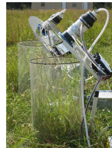
Figure 1. The photo above shows a pair of flux chambers at the field site in the Duke Forest.
2.5 Flux-chamber description
The dynamic flux chambers, which are shown in Fig. 1, were constructed using clear, cylindrically shaped acrylic. The chambers were constructed in pairs, and each pair had an open-bottomed chamber, which measured deposition to the vegetation inside, and a “blank” chamber, which had an acrylic bottom, and enabled us to measure deposition in the absence of vegetation. The blank measurement represents trace-gas losses to the chamber walls as well as any chem-ical reactions in the chamber that are unaccounted for in the flux calculations.
All of the chambers have a 45.7 cm diameter and 0.48 cm wall thickness. Four pairs of chambers have a height of 83.8 cm, and the remaining pair has a height of 58.4 cm. The chambers were designed with this height distribution because many species of natural vegetation, including grassland, are taller than 58.4 cm. The shorter chambers were designed to measure fluxes over shorter vegetation, such as alpine tundra, which is present in sensitive areas like Rocky Mountain Na-tional Park. The shorter chambers are likely more accurate for vegetation below 59 cm tall, since they increase the ratio of vegetative surface area to volume.
Air Outlet to small pump (5 L/min), which pulls air over control board and inexpensive sensors
Air Outlet to O3, NOx, H2O, and CO2 monitors Outlet: Main Vacuum
Pump (80 L/min)
Automated lid
Air Inlet Air Inlet
12.5 cm long spacer for #10 socket haed cap screw
46.67 ST OCK
10.16 STOCK PVC PIPE
0.47 STOCK
8
5.20
10.16 83.80
20.32
12.5 cm long spacer for!
#10 socket head cap screw!
Figure 2. The plot above shows the dimensions of the chamber and the locations of the air inlets and outlet.
top of the chamber, as shown in Fig. 2. The grass outside the chamber, near the inlet holes, is removed, which prevents trace gases from depositing to external vegetation before the air stream enters the chamber.
Air is pulled through the chamber by a US General 3 CFM Two-Stage Vacuum Pump, and concentration samples were measured in one of two polytetrafluoroethylene (PTFE) tubes at the outlet. Gas-phase sampling is discussed in more detail in Sect. 2.6.
For most experiments, the pump was set to pull 80 L min−1 of air through the chamber. In addition to the flow induced by the vacuum pump, the 2B ozone monitor pulled ap-proximately 1 L min−1; the Thermo Scientific NOxanalyzer
pulled 0.1 L min−1; the LI-COR H2O/CO2monitor pulled
0.25 L min−1; and the small, inexpensive pump, which pulled air over the inexpensive sensors, pulled 5 L min−1. Thus, the total flow rate through the chamber was 86.35 L min−1, which equates to a residence time of 1.5 min. Pape et al. (2009) found that other researchers have operated dynamic flux chambers with residence times ranging from 10 s to 24 min and chose to operate their dynamic flux chambers at a residence time of 40 s (Pape et al., 2009). Gillis and Miller
(2000) found that changes in air-stream residence time in flux chambers caused proportional changes in mercury flux for both absorption and emission (Gillis and Miller, 2000). Aeschlimann and coworkers used a residence time of 15 s during the day and 60 s at night (Aeschlimann et al., 2005), which reflects ambient diurnal variation in friction velocity. Low residence times ensure that chambers are well mixed and minimize reactions between gases in the chamber. How-ever, reducing residence times also reduces the difference in ambient and steady-state trace-gas concentrations in the chamber. Thus, as residence time is decreased, more precise instrumentation is required. We chose to operate our cham-bers with a 1.5 min residence time, because 1.5 min is suf-ficiently low to keep environmental conditions close to am-bient yet still yield a trace-gas concentration change that is large enough to be detected by inexpensive sensors. This res-idence time also translates to a flow rate that can be generated with an inexpensive pump.
Another way that we reduced the cost of the chamber was by designing our own control system, using inexpen-sive electronic components. A customized embedded-system platform was used to automate the flux-chamber sampling system. The system is based on the low-cost M-Pod air qual-ity monitor (Masson, 2014), with additional instrumentation for pump and actuator control. Firmware running on the com-mon Atmel (San Jose, CA) Atmega 328 microcontroller con-trols both the data logging and flux-chamber sampling rou-tine.
Each chamber runs approximately once an hour, and the main vacuum pump is off when the chamber is not sampling. Once per hour, a predefined and automated sampling sched-ule begins, and the vacuum pump turns on and runs with the lid open for 6.75 min. The pressure change caused by the pump can cause fluctuations in instrument readings, and this boot-up time allows the instruments to stabilize before the chamber lid closes. After the 6.75 min initialization, the chamber lid closes and remains closed for 5 min. It is impor-tant to note that the eddy-covariance measurements are fluxes averaged over a 30 min or 1 h time period, and the chamber measurements are a 5 min average, taken every 53 min.
Fluxes were calculated based on the assumption that the chamber was well mixed. A mass balance in the chamber yields the equation
Vdµj(t )
dt =Qµj,amb−Qµj(t )−FjAs, (1)
whereµj(t )is the mixing ratio in the chamber of gas,j, with
respect to time;Qis the flow rate of air through the chamber;
µj,ambis the ambient mixing ratio of gas,j;t is time;Asis
the surface area of the opening at the bottom of the chamber;
V is volume of the chamber; andFj is the flux of gas,j, to
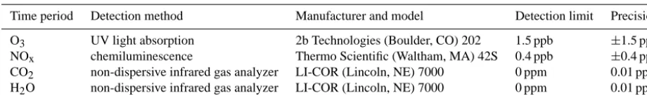
Table 2. Trace gas detectors used in this study, with manufacturers’ specifications.
Time period Detection method Manufacturer and model Detection limit Precision
O3 UV light absorption 2b Technologies (Boulder, CO) 202 1.5 ppb ±1.5 ppb
NOx chemiluminescence Thermo Scientific (Waltham, MA) 42S 0.4 ppb ±0.4 ppb
CO2 non-dispersive infrared gas analyzer LI-COR (Lincoln, NE) 7000 0 ppm 0.01 ppm H2O non-dispersive infrared gas analyzer LI-COR (Lincoln, NE) 7000 0 ppm 0.01 ppm
µj(t )=µj,amb−
FjAs
Q (1−e
−Q
Vt). (2)
The steady-state solution to this equation, solving for flux, is
F = Q
As
(µj,amb−µj(τss)), (3)
whereτssis the time when the trace-gas concentration in the
chamber reaches steady state. 2.6 Gas-phase measurements
Figure 2 shows the flow path of sample air through the cham-ber. Gas-phase measurements were conducted at the chamber outlet, which consisted of an 11.4 cm diameter PVC pipe. Chamber air was pulled through the outlet via the main vac-uum pump. Two 4.76 mm diameter tubes were attached to the sides of the PVC pipe on one end, and instruments on the other. One tube was connected to a 2B Technologies Model 202 Ozone Monitor, Thermo Scientific Model 42S NOx
ana-lyzer, and LI-COR 7000 H2O/CO2monitor. More
informa-tion about the instruments is available in Table 2.
The second tube was connected to a small vacuum pump, which moved air through the chamber control box. In addi-tion to the control board, the box housed metal-oxide NOx
and O3sensors. Additional data were collected using these
commercially available sensors, specifically the Sensortech (Chemlsford, UK) (formerly e2v) MICS-2611 O3sensor. All
low-cost sensors implemented in the flux-chamber system ranged in cost from USD 10 to 100, and the O3sensors had
a detection limit well within typical concentration changes seen in ground-flux measurements. Complex quantification schemes are necessary to quantify the sensor output properly. Such schemes incorporate correction parameters for interfer-ence effects. Inexpensive sensor technology has the poten-tial to be incorporated into a flux-chamber system effectively, which would make widespread flux measurements a realiz-able objective.
2.7 Comparison of eddy-covariance and flux-chamber measurements
Theoretically, dry deposition flux (F) is proportional to the ambient concentration (C) of a trace gas at some reference height (Seinfeld and Pandis, 2006). The proportionality con-stant between the concentration and flux is called “deposition velocity” (vd) (Chamberlain and Chadwick, 1953), and
F = −vdC. (4)
The deposition process has been described using a resistance analogy (Wesely and Hicks, 2000), in which species trans-port from the atmosphere to the surface of a material is con-trolled by three resistances in series.
vd=
1
rt
= 1
ra+rb+rc
, (5)
wherertis the total resistance to deposition,rais the
resis-tance to aerodynamic transport,rbis the resistance to
diffu-sion through the quasi-laminar boundary layer, andrc is the
resistance to uptake of a trace gas by the canopy.
This resistance analogy is based on the assumption that the atmosphere is unaltered. It is an accurate analogy for eddy-covariance measurements, but flux chambers alter the wind speed above the canopy, so the resistance analogy must be adjusted. Pape et al. (2009) proposed an alternate resistance scheme, which replacesrawithrpurgeandrmix, which
repre-sent the purging resistance between ambient and chamber air, and mixing in the chamber, respectively. When the chamber is well mixed,rmixis very small, and it can therefore be
ne-glected in this case.rbis replaced with a modified
boundary-layer resistance,rb∗.rc should be modified very little by the
chamber, provided the chamber does not substantially alter the environmental conditions (temperature, relative humid-ity) of the natural environment.
Thus, the ratio of chamber flux to ambient flux can be writ-ten as
Fcham
Famb
= ra+rb+rc
rpurge+rb∗+rc
. (6)
In order to findrpurge+rb∗, we conducted an experiment,
20:57 20:58 21:00 21:01 21:02 21:04 21:05 21:07 21:08 21:10 0
2 4 6 8 10 12 14 16 18 20
Time of Day
Ozone Concentration (ppb)
vacuum pump pulls air through the chamber, and ozone concentration increases at an unrealistic rate
lid closes and concentration in chamber drops
concentration in chamber approaches steady state
Figure 3. The plot above is an example of a run where the data could not be used to calculate a flux. The ozone concentration increases by an unreasonable amount when the chamber lid opens, which likely indicated malfunction in the 2B ozone monitor.
sink, sorc can be approximated as zero (Galbally and Roy,
1980) in this experiment. We used the equation
vd=
1
rpurge+rb∗+rc
(7) and the measured deposition velocity from the KI experiment to calculaterpurge+rb∗(rpurge+rb∗=1/vd=57.5 s m−1). The
value ofrpurge+rb∗describes aerodynamic and quasi-laminar
boundary-layer resistance to deposition inside the chamber, so, while ozone was used to find the value, it is applicable to all gases. For future researchers, we would suggest repeating this experiment with different flow and vegetation character-istics.
We present both measured ozone fluxes and values ad-justed using this resistance analogy. While this conversion factor enables chamber flux to be scaled to ambient flux, it introduces modeling assumptions and additional uncertainty to an otherwise direct measurement.
3 Results and discussion 3.1 Data processing
We collected O3 flux data for 8 days. We used two pairs
of identical tall chambers and one pair of shorter chambers. Each set of data was based on a 5-minute chamber closure, which occurred once per hour. The flux during each sampling period was assumed to be constant. Each data run was ana-lyzed for noise and pattern, and some data sets were excluded from results.
Figure 3 is an example of a sampling period that we ex-cluded from our results. The ozone concentration increased
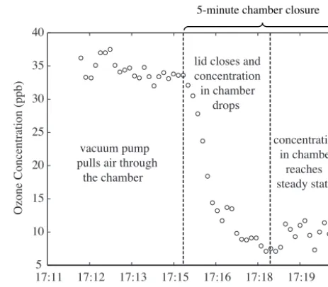
17:115 17:12 17:13 17:15 17:16 17:18 17:19 17:21 10
15 20 25 30 35 40
lid closes and concentration in chamber drops
vacuum pump pulls air through the chamber
concentration in chamber reaches steady state
Time of Day
Ozone Concentration (ppb)
5-minute sampling period!
5-minute chamber closure!
Figure 4. The plot above is an example of ozone data that can be analyzed using the steady-state mass-balance equation. The data be-fore the lid is closed and at the end of the sample both have low noise and stay relatively constant for at least 1 min.
by an unreasonable amount when the chamber lid opened, which likely indicates malfunction in the 2B ozone moni-tor. Nine percent of chamber A data were excluded, 11 % of chamber B data were excluded, and 0 % of the chamber C data were excluded.
Figure 4 shows the ozone concentration in the chamber during one sampling period, as an example of ozone data that can be analyzed using the steady-state solution. The area before the decline of the ozone concentration represents the time period when the chamber lid was open. After the lid closed, the concentration began to decline and eventu-ally reached a steady-state value. This data set met our data-quality requirements, as the data just before the lid closed and at the end of the sample both have low noise and stay relatively constant for at least 1 min. Therefore, the flux was computed using the steady-state solution (Eq. 3).
In addition to the data selection mentioned above, we also looked for short-term extreme fluctuations in the ozone time series. The first step in this process was to calculate rolling 1 min averages. Next, we found the standard deviation of the six concentration values used to calculate each 1 min aver-age. We excluded the 1 min averages with a standard devia-tion greater than 3 ppb. This value was chosen because, when we looked at a histogram of the standard deviations, values greater than 3 ppb were outliers. This data-quality-check pro-cess resulted in the removal of 1.4 % of the 1 min average data.
ozone concentration for each cycle by calculating the mean of the last 2 min of concentration data before the chamber lid closed. We found the steady-state concentration by cal-culating the mean of the data between 3 and 5 min after the chamber closed. Finally, we used the ambient and steady-state concentrations we found for each data set to compute flux, using Eq. (7).
When the ambient ozone concentration is below 5 ppb, we assume that the ozone flux is zero. Ambient O3
concentra-tions of 5 ppb or lower typically occur only at night, when wind speeds are low, which means that the aerodynamic re-sistance to deposition is high, equating to a low flux. The absolute highest flux rate that could occur, with an ambient concentration of 5 ppb, is 0.09 µg m−2s−1(from Eq. 3), and a flux rate this high is very unlikely with low wind speeds. The median ozone-flux rate measured via eddy covariance, when the ambient ozone concentration was≤5 ppb, during the eight-day sampling period was 0 µg m−2s−1, with a
stan-dard deviation of 0.05 µg m−2s−1.
We did not use the blank chamber data to make any ad-justments to the fluxes measured by the dynamic cham-bers. The median difference between ambient concentration and steady-state ozone concentration was 1.9 ppb for the blank chambers. Since the uncertainty in ozone concentra-tions measured by the 2B ozone monitor is ±1.5 ppb, the concentration difference is within a 95 % confidence inter-val for noise. Thus, correcting chamber fluxes for blank flux would only introduce more error into our measurements.
Also, the median flux measured by the blank cham-bers, when the open-bottom-chamber flux was nonzero, was −0.001 µg m−2s−1. This value is less than 1 % of the
me-dian of the nonzero open-bottom-chamber fluxes, which was −0.21 µg m−2s−1. Therefore, correcting for the blank
cham-ber fluxes would not have a significant impact on measure-ments. It was encouraging that the blank fluxes were so small, since this indicated that wall losses do not have a significant impact on the flux-chamber measurements. Since wall losses were insignificant, the chamber design could be further simplified by eliminating the blank chambers. 3.2 Photochemistry in the chamber
Photochemical reactions between NO, NO2, and O3can
oc-cur in the chamber and therefore must be considered in Eq. (1) (Meixner et al., 1997; Pape et al., 2009). The primary reactions of concern are
NO+O3→NO2+O2 (R1)
and NO2+hv
O2
→NO+O3, λ<420 nm. (R2)
Pape and coworkers measuredj (NO2)inside their
cham-ber and found that the average value of j (NO2)inside the
chamber was 48 % of the value outside the chamber (Pape
Date
Ozone Flux (ug/m2/s)
09/22 09/23 09/24 09/25 09/26 09/27 09/28
−0.1 0 0.1 0.2 0.3 0.4 0.5 0.6
Cham. A Eddy Cov. Cham. B Cham. C Model
O
zo
ne
F
lu
x
R
at
e
(
g
m
-2s -1)
µ
Chamber A in high LAI location
Chamber A moved to average LAI location
Date
Ozone Flux (ug/m2/s)
09/22 09/23 09/24 09/25 09/26 09/27 09/28
−0.1 0 0.1 0.2 0.3 0.4 0.5 0.6
Cham. A Eddy Cov. Cham. B Cham. C Model
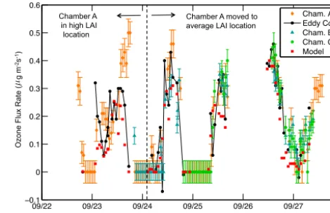
Figure 5. The plot above compares O3fluxes measured using eddy covariance (solid black line and black dots); surface-exchange mod-eling (red squares); and flux chambers A (orange diamonds), B (blue triangles), and C (green circles). The error bars represent the 95 % confidence interval. The tick marks represent midnight on the date listed.
et al., 2009). They fit a curve ofj (NO2)vs. global radiation
(G), and we used that curve in our calculations, since our chambers were similar in shape and material. To quantify the impact of this assumption, we calculated how increas-ing and decreasincreas-ingj (NO2)by 25 % affects ozone flux and
found that this changes ozone flux by<1 % in all cases. The maximum flux change due to photolysis in all of our results is 1.7 %. Thus, the impact of photolysis on ozone flux was small during our study. More information about our calcula-tion of photolysis rate can be found in the Supplement. 3.3 Ozone results
We measured ozone dry deposition with flux chambers for 2 days in June, and 8 days in September. When compared with eddy-covariance measurements, flux-chamber ozone mea-surements were able to capture the diurnal flux trends. It is important to remember that eddy-covariance measurements are not without error. For an eddy-covariance system simi-lar to the one used in this study, Finkelstein and Sims (2001) found that mean sampling errors for 30 min average eddy-covariance O3fluxes were in the range of 27–33 %.
Figure 5 shows O3 fluxes measured via eddy covariance
and flux chambers A, B and C, and also calculated using an indirect method, which combined meteorological data and surface-exchange model for the time period between 22 and 28 September. The theory used to calculate the model val-ues is described by Wesely (1989) and Seinfeld and Pandis (2006).
al-Figure 6. Chamber A (left). Chamber B (right). The vegetation in chamber A, prior to being moved on 24 September, was not repre-sentative of the typical vegetation type or LAI at the site. As a result, flux measurements prior to the move were large when compared with measurements from other chambers and eddy covariance. The vegetation in chamber B was representative of the vegetation in the field.
ways predict flux accurately (Wu et al., 2012; Schwede et al., 2011).
Chamber A was moved from its original location in the field to a different position on 24 September. Prior to be-ing moved, the chamber was on a plot of land with a less-prevalent vegetation type, which had a higher LAI than the dominant vegetation (see Fig. 6). After the chamber was moved to a location with more representative vegeta-tion, the data matched the eddy-covariance results much bet-ter. Before the chamber was moved (18 and 23 Septem-ber), the mean ozone-flux rate measured by eddy covari-ance was −0.16 µg m−2s−1, and the mean chamber flux
rate was −0.23 µg m−2s−1, which is 48 % higher than
the eddy-covariance measurement. After the move (24– 27 September), the mean eddy-covariance flux rate was −0.25 µg m−2s−1, and the mean flux measured by the chamber was −0.26 µg m−2s−1, which is 4 % higher than the eddy-covariance measurement. This difference in mea-surement agreement highlights the importance of selecting a chamber placement that contains vegetation representative of the footprint of the eddy-covariance tower.
Chamber B operated from 18 to 19 September, and again from 23 to 27 September. The mean ozone flux measured by the flux chamber during this period was−0.17 µg m−2s−1, which is 9 % higher than the mean eddy-covariance ozone flux during the same period (−0.15 µg m−2s−1).
Chamber C, which is the shorter chamber, was operated between 18 and 19 September, and again between 24 and 27 September. The mean chamber flux measured during this period was −0.115 µg m−2s−1, which was 6 % lower than the mean eddy-covariance flux during the same time period (−0.108 µg m−2s−1).
In addition to the September measurements, data were collected for 4 days in June. The chambers underestimated ozone flux by 50–100 % in June, and we believe that this was because the LAI was much lower in the chambers than in the
field during that time. Because we did not anticipate the spa-tial and temporal variability in LAI, nor its subsequent im-pact on flux measurements, we did not measure LAI during our June sampling period. However, we estimate, by visual inspection, that LAI in the chambers was about 50 % lower in June than in September. Further studies that measure ozone deposition with various known LAI values in the chamber could confirm the effects of changing LAI on measured flux. We will measure LAI in all future flux experiments.
There was not a systemic bias in the ozone flux data. The excellent agreement between the September flux-chamber and eddy-covariance measurements demonstrates that the flux chamber is capable of measuring ozone flux to grassland ecosystems when the LAI inside the chamber represents the average LAI in the field.
3.4 Chamber versus eddy-covariance regression analysis
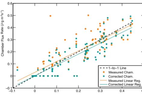
Plot 7 shows a regression analysis of measured chamber flux rates and chamber flux rates that are adjusted using the chamber-to-ambient flux rate correction versus eddy co-variance. While this plot is interesting, we need to be care-ful about placing too much emphasis on these results, since the averaging times were different for the eddy covariance (averaged over a 1 h period) and chamber measurements (5 min average). It is also important to remember that the eddy-covariance measurements have uncertainty, which Fin-klestein and Sims found to be 30%, on average, for half-hourly fluxes (Finkelstein and Sims, 2001).
Linear regressions were found for the measured and cor-rected chamber data versus eddy-covariance data. The mea-sured data had a slope of 0.89 and an intercept of 0.03, with a coefficient of determination (R2) of 0.64. With 95 % confidence, the slope is significantly different than 1 (pvalue = 5.8×10⁻²⁴), and the intercept is not significantly different than 0 (pvalue=0.55), although it is worth noting that the intercept would be significantly different than zero at a slightly higher confidence interval.
Linear regression between the corrected chamber and eddy-covariance data yielded a slope of 0.90 and an intercept of 0.002, with anR2of 0.77. With 95 % confidence, the slope is significantly different than 1 (p value=51.3×10⁻³³), and the intercept is not significantly different than zero (p value=0.89). While the corrected data has a slope closer to 1 and an intercept closer to 0 than the measured data, the two lines are not significantly different in slope (p value=0.92) or intercept (p value=0.91). Perhaps a more important result of the correction is that it pulled the 2 most extreme chamber flux values (both−0.5 µ g m−2s−1), closer to agreement with the eddy-covariance values; this is reflected in the increased value ofR2.
Eddy Covariance Flux
Chamber Flux
−0.1 0 0.1 0.2 0.3 0.4 0.5
−0.1 0 0.1 0.2 0.3 0.4 0.5 0.6
1−to−1 Line Raw Cham. Flux Corrected Cham. Flux Raw Linear Reg. Corrected Linear Reg.
Rate ( g m-2s-1) Eddy Covariance Flux
Chamber Flux
−0.1 0 0.1 0.2 0.3 0.4 0.5
−0.1 0 0.1 0.2 0.3 0.4 0.5 0.6
1−to−1 Line Raw Cham. Flux Corrected Cham. Flux Raw Linear Reg. Corrected Linear Reg.
R
at
e
(
g
m
-2s -1)
µ
µ
Measured Cham. Corrected Cham. Measured Linear Reg.
Figure 7. The plot above is a comparison of ozone fluxes measured using flux chambers with fluxes obtained via eddy covariance. The orange dots represent fluxes measured by the chambers, and the blue dots represent chamber fluxes that have been corrected using the adjusted resistance analogy. The dashed line is a 1-to-1 line. The orange line represents a linear regression of the measured cham-ber fluxes, and the blue line is a linear regression of the corrected chamber fluxes.
the corrected chamber data. While the mean of the corrected chamber flux rate is 9 % farther from the eddy covariance than the measured chamber flux rate, both are well within the uncertainty of the eddy-covariance measurements. Based on the reduction of extreme values and increasedR2, we believe that performing the correction improves the chamber results overall.
3.5 Seasonal flux and implications for chamber flux measurements
We completed this validation work in September, which demonstrates chamber performance in the late summer/early fall. In order to predict chamber performance in other seasons, we used seasonal meteorological data from the Duke Forest to calculate typical values of ra, rb, and rc
as well as the chamber-to-ambient flux correction factors (Fcham/ Famb) for winter, spring, summer, and fall. The
me-teorological data set includes air temperature, wind speed, friction velocity, relative humidity, global radiation, and rain-fall information from 2013. We chose 1 week of represen-tative data for each season (6–12 February, 21–27 April, 2–8 August, 2–8 November). We used a surface-exchange model, combined with the meteorological data, to calculate
ra,rb, and rc. The model is based on the theory in Wesely
(1989) and Seinfeld and Pandis (2006). A constant value of 57.5 s m−1was used forrpurge+rb∗(see Sect. 2.7 for details
on the calculation ofrpurge+rb∗).
As shown in Table 3, the aerodynamic (ra) and
quasi-laminar boundary-layer (rb) resistances are similar in all
seasons. The overall median canopy resistance is lowest in the summer (110 s m−1), slightly higher in the spring
(147 s m−1), higher still in the fall (263 s m−1), and
drasti-cally higher in the winter (1348 s m−1). In the spring,
sum-mer, and fall, the canopy resistance makes up approximately 50 % of the total resistance to deposition, whereas in the win-ter it contributes 90 % of the total deposition resistance. This discrepancy in canopy resistance results in seasonal variabil-ity of the chamber-to-ambient flux correction factors. The range of correction factors (5th to 95th percentile) is much larger in the spring (0.86–2.89), summer (0.87–2.82), and fall (0.92–2.84) than in the winter (0.99–1.35).
At night, the correction factor is typically greater than 1, which has the effect of reducing the flux measured by the chamber. This accounts for the fact that the turbulence in the chamber may exceed the ambient turbulence at night. The magnitude of the nighttime correction factor is reduced in the winter as a result of the very large canopy resistance, which is so dominant that differences in aerodynamic conditions are inconsequential. During the day, the typical correction factor is close to 1 in all seasons, and sometimes below 1, which means that the turbulence in the chamber during the day typ-ically matches the ambient conditions well but can be lower or higher than ambient at any given time.
Our validation experiments were conducted in late sum-mer/early fall. Since the chamber-to-ambient correction fac-tors vary the most in the spring, summer, and fall, we have demonstrated that chambers can accurately predict flux when the turbulence in the chambers differs from ambient. Due to the dominance of canopy resistance in the winter, aerody-namic differences should be negligible at that time of year. In addition to correction factors, it is important to consider overall median deposition velocities, which are greatest in the spring and summer (−0.35 and−0.32 cm s−1), slightly
lower in the fall (−0.27 cm s−1), and very low in the
Table 3. Seasonal mean resistance, correction factor, and deposition Velocity.
Winter Spring Summer Fall
medianvd(cm s−1) 0.07 0.35 0.32 0.27
medianra(s m−1) 56 45 71 67
medianrb(s m−1) 21 20 38 30
Overall medianrc(s m−1) 1348 147 110 263
medianFcham/ Famb 1.01±0.02 1.02±0.9 1.20±0.74 1.12±1.0
95th percentileFcham/ Famb 1.35 2.89 2.82 2.84
5th percentileFcham/ Famb 0.99 0.86 0.87 0.92
medianvd(cm s−1) 0.11 0.56 0.63 0.38
medianra(s m−1) 39 30 35 33
medianrb(s m−1) 15 13 21 16
Daytime medianrc(s m−1) 876 130 103 209
medianFcham/ Famb 1.00±0.02 0.94±0.31 0.99±0.53 0.97±0.66
95th percentileFcham/ Famb 1.03 1.53 1.47 1.25
5th percentileFcham/ Famb 0.98 0.84 0.84 0.91
medianvd(cm s−1) 0.05 0.25 0.23 0.22
medianra(s m−1) 91 101 145 128
medianrb(s m−1) 32 44 77 56
Nighttime medianrc(s m−1) 1348 245 255 282
medianFcham/ Famb 1.04±0.04 1.31±1.14 1.57±0.74 1.38±1.1
95th percentileFcham/ Famb 1.44 3.65 3.24 3.1
5th percentileFcham/ Famb 1.0 0.97 1.06 1.0
4 Conclusions
Ozone deposition onto a grassland ecosystem was measured using dynamic flux chambers and eddy covariance. Ozone-deposition measurements from the two methods matched very well (4–10 % difference) when the LAI inside the cham-bers was representative of the average LAI in the field. This discrepancy is within the uncertainty of eddy covariance, and the flux chambers are considered an accurate measure-ment system under these conditions. There was not a bias in the chamber data, when compared with the eddy-covariance data.
When LAI inside the chambers was significantly higher or lower than the rest of the field, chamber measurements over- or underpredicted flux, respectively. A discrepancy be-tween chamber and average LAI values can be caused by both inconsistency in vegetation density and differences in vegetation species. Eddy-covariance systems can only mea-sure net flux to an entire fetch (>100 m2), which means that they measure a mean flux to all vegetation in the field and cannot measure flux to small patches of different vegetation types. Flux chambers are able to measure flux onto different patches of vegetation, which enables the user to understand the relative contribution of different vegetation species to to-tal flux.
In this work, our strategy was to place every chamber on a plot of vegetation that represented the average vegetation in the field. This enabled us to confirm that the results were
consistent between chambers. In the field at the Duke Forest, the minority vegetation types represent such a small fraction of the overall grassland that it is very unlikely they have a large net effect on the flux.
It would be very interesting, in future work, to intention-ally place the chambers over different types of vegetation in a field and attempt to quantify what percentage of the vege-tation each plot represents, and then use a weighted average of ozone fluxes onto the five types of vegetation to estimate the overall flux.
We found that the median ozone flux measured by the blank chambers, when the open-bottom-chamber flux was nonzero, was−0.001 µg m−2s−1. This value is less than 1 % of the median of the nonzero open-bottom-chamber fluxes, which was−0.21 µg m−2s−1. Therefore, we can conclude that we achieved the design goal of minimizing trace-gas in-teractions with the walls of the chamber.
CO2 measurements were conducted for one 20 h period,
and the flux chamber captured the diurnal trend in CO2flux.
The quantity of the data was not sufficient to validate cham-ber performance, but the results show promise, and addi-tional experiments will be conducted to confirm that the flux chambers can measure CO2deposition accurately.
Flux-chamber NOx measurements were conducted for 4
days. Unfortunately, the eddy-covariance system for mea-suring NOxwas not available during this field campaign, so
comparisons could not be made. However, NOxfluxes
for the site. Additional experiments will be performed to con-firm that the chamber NOx-flux measurements are accurate.
The ultimate goal of our research is to operate the cham-bers with inexpensive sensors, and the next phase of the project is to validate performance for these sensors. Future work will also consist of measuring different species and us-ing the chambers to measure spatial variability in dry depo-sition.
The Supplement related to this article is available online at doi:10.5194/amt-8-267-2015-supplement.
Acknowledgements. We are grateful for the opportunity to do this
work, which was funded by the Electric Power Research Institute (EPRI). We would like to thank Corey Miller for his help building the flux chambers. We would like to thank Peter Hamlington, Nick Clements, Bill Mitchell, and Andrew Turnipseed for helpful discussions. This project would not have been possible without equipment borrowed from Christine Wiedinmyer and John Ortega, at the National Center for Atmospheric Research, as well as Joanna Gordon and Ashley Collier. Ricardo Piedrahita and Nick Masson’s sensor work is the basis for the inexpensive sensor portion of this project.
Disclaimer. This document has been reviewed in accordance
with US Environmental Protection Agency policy and approved for publication. The views expressed in this article are those of the author[s] and do not necessarily represent the views or policies of the US Environmental Protection Agency.
Edited by: T. F. Hanisco
References
Aeschlimann, U., Nösberger, J., Edwards, P. J., Schneider, M. K., Richter, M., and Blum, H.: Responses of net ecosystem CO2 ex-change in managed grassland to long-term CO2enrichment, N fertilization and plant species, Plant Cell Environ., 28, 823–833, 2005.
Altimir, N., Vesala, T., Keronen, P., Kulmala, M., and Hari, P.: Methodology for direct field measurements of ozone flux to fo-liage with shoot chambers, Atmos. Environ., 36, 19–29, 2002. Baldocchi, D. D., Hincks, B. B., and Meyers, T. P.: Measuring
biosphere–atmosphere exchanges of biologically related gases with micrometeorological methods, Ecology, 69, 1331–1340, 1988.
Benedict, K. B., Day, D., Schwandner, F. M., Kreidenweis, S. M., Schichtel, B., Malm, W. C., and Collett Jr., J. L.: Observations of atmospheric reactive nitrogen species in Rocky Mountain Na-tional Park and across northern Colorado, Atmos. Environ., 64, 66–76, 2013.
Breuninger, C., Oswald, R., Kesselmeier, J., and Meixner, F. X.: The dynamic chamber method: trace gas exchange fluxes (NO, NO2, O3) between plants and the atmosphere in the laboratory and in the field, Atmos. Meas. Tech., 5, 955–989, doi:10.5194/amt-5-955-2012, 2012.
Breuninger, C., Meixner, F. X., and Kesselmeier, J.: Field in-vestigations of nitrogen dioxide (NO2) exchange between plants and the atmosphere, Atmos. Chem. Phys., 13, 773–790, doi:10.5194/acp-13-773-2013, 2013.
Brook, J. R., Zhang, L., Di-Giovanni, F., and Padro, J.: Description and evaluation of a model of deposition velocities for routine es-timates of air pollutant dry deposition over North America: Part I: model development, Atmos. Environ., 33, 5037–5051, 1999. Chamberlain, A. and Chadwick, R. C.: Deposition of airborne
ra-dioiodine vapour, Nucleonics, 11, 22–25, 1953.
DeHayes, D. H., Schaberg, P. G., Hawley, G. J., and Strimbeck, G. R.: Acid rain impacts on calcium nutrition and forest health alteration of membrane-associated calcium leads to membrane destabilization and foliar injury in red spruce, BioScience, 49, 789–800, 1999.
Driscoll, C. T., Lawrence, G. B., Bulger, A. J., Butler, T. J., Cro-nan, C. S., Eagar, C., Lambert, K. F., Likens, G. E., Stod-dard, J. L., and Weathers, K.: Acidic Deposition in the Northeast-ern United States: Sources and Inputs, Ecosystem Effects, and Management Strategies: The effects of acidic deposition in the northeastern United States include the acidification of soil and water, which stresses terrestrial and aquatic biota, BioScience, 51, 180–19, 2001.
EPA US: Clean Air Status and Trends Network 2010 Annual Re-port, Tech. rep., AMEC Environment & Infrastructure, Inc, pre-pared for US EPA Under Contract No. EP-W-09-028, 2010. Fangmeier, A., Hadwiger-Fangmeier, A., Van der Eerden, L., and
Jäger, H.-J.: Effects of atmospheric ammonia on vegetation – a review, Environ. Pollut., 86, 43–82, 1994.
Fenn, M. E., Poth, M. A., Aber, J. D., Baron, J. S., Bormann, B. T., Johnson, D. W., Lemly, A. D., McNulty, S. G., Ryan, D. F., and Stottlemyer, R.: Nitrogen excess in North American ecosys-tems: predisposing factors, ecosystem responses, and manage-ment strategies, Ecol. Appl., 8, 706–733, 1998.
Finkelstein, P. and Sims, P.: Sampling error in eddy correlation flux measurements, J. Geophys. Res., 106, 3503–3509, 2001. Flechard, C. R., Nemitz, E., Smith, R. I., Fowler, D.,
Ver-meulen, A. T., Bleeker, A., Erisman, J. W., Simpson, D., Zhang, L., Tang, Y. S., and Sutton, M. A.: Dry deposition of reactive nitrogen to European ecosystems: a comparison of in-ferential models across the NitroEurope network, Atmos. Chem. Phys., 11, 2703–2728, doi:10.5194/acp-11-2703-2011, 2011. Fluxnet: Duke Forest Open Field, available at: http://fluxnet.ornl.
gov/site/867 (last access: 14 December 2013), 2013.
Foken, T. and Wichura, B.: Tools for the quality assessment of surface-based flux measurements, Agr. Forest Meteorol., 78, 83– 105, 1996.
Galbally, I. E. and Roy, C. R.: Destruction of ozone at the earth’s surface, Q. J. Roy. Meteor. Soc., 106, 599–620, 1980.
Geßler, A., Rienks, M., and Rennenberg, H.: NH3and NO2fluxes between beech trees and the atmosphere–correlation with cli-matic and physiological parameters, New Phytol., 147, 539–560, 2000.
Gillis, A. and Miller, D. R.: Some potential errors in the measure-ment of mercury gas exchange at the soil surface using a dynamic flux chamber, Sci. Total Environ., 260, 181–189, 2000.
Gut, A., Van Dijk, S., Scheibe, M., Rummel, U., Welling, M., Ammann, C., Meixner, F., Kirkman, G., Andreae, M., and Lehmann, B.: NO emission from an Amazonian rain forest soil: continuous measurements of NO flux and soil concen-tration, J. Geophys. Res.-Atmos., 107, LBA 24-1–LBA 24-10, doi:10.1029/2001JD000521, 2002.
Horst, T.: A simple formula for attenuation of eddy fluxes measured with first-order-response scalar sensors, Bound.-Lay. Meteorol., 82, 219–233, 1997.
Horst, T. and Weil, J.: How far is far enough? The fetch require-ments for micrometeorological measurement of surface fluxes, J. Atmos. Ocean. Tech., 11, 1018–1025, 1994.
Horváth, L., Führer, E., and Lajtha, K.: Nitric oxide and nitrous oxide emission from Hungarian forest soils; linked with atmo-spheric N-deposition, Atmos. Environ., 40, 7786–7795, 2006. Kaimal, J. and Finnigan, J.: Atmospheric Boundary-Layer Flows:
Their Structure and Measurement, Oxford University Press, 1994.
Kirkman, G., Gut, A., Ammann, C., Gatti, L., Cordova, A., Moura, M., Andreae, M., and Meixner, F.: Surface exchange of nitric oxide, nitrogen dioxide, and ozone at a cattle pasture in Rondonia, Brazil, J. Geophys. Res.-Atmos., 107, LBA 51-1– LBA 51-17, doi:10.1029/2001JD000523, 2002.
Kitzler, B., Zechmeister-Boltenstern, S., Holtermann, C., Skiba, U., and Butterbach-Bahl, K.: Nitrogen oxides emission from two beech forests subjected to different nitrogen loads, Biogeo-sciences, 3, 293–310, doi:10.5194/bg-3-293-2006, 2006. Li, Y., Aneja, V. P., Arya, S., Rickman, J., Brittig, J., Roelle, P., and
Kim, D.: Nitric oxide emission from intensively managed agri-cultural soil in North Carolina, J. Geophys. Res.-Atmos., 104, 26115–26123, 1999.
Masson, N.: UPOD: An open-source platform for air quality mon-itoring, available at: http://mobilesensingtechnology.com/ (last access: 10 January 2014), 2014.
Meixner, F., Fickinger, T., Marufu, L., Serca, D., Nathaus, F., Mak-ina, E., Mukurumbira, L., and Andreae, M.: Preliminary results on nitric oxide emission from a southern African savanna ecosys-tem, Nutr. Cycl. Agroecosys., 48, 123–138, 1997.
Muller, J. B. A., Percival, C. J., Gallagher, M. W., Fowler, D., Coyle, M., and Nemitz, E.: Sources of uncertainty in eddy co-variance ozone flux measurements made by dry chemilumines-cence fast response analysers, Atmos. Meas. Tech., 3, 163–176, doi:10.5194/amt-3-163-2010, 2010.
Musselman, R. C., Lefohn, A. S., Massman, W. J., and Heath, R. L.: A critical review and analysis of the use of exposure and flux-based ozone indices for predicting vegetation effects, Atmos. En-viron., 40, 1869–1888, 2006.
Norman, J., Kucharik, C., Gower, S., Baldocchi, D., Crill, P., Ray-ment, M., Savage, K., and Striegl, R.: A comparison of six meth-ods for measuring soil-surface carbon dioxide fluxes, J. Geophys. Res.-Atmos., 102, 28771–28777, 1997.
Pape, L., Ammann, C., Nyfeler-Brunner, A., Spirig, C., Hens, K., and Meixner, F. X.: An automated dynamic chamber system for surface exchange measurement of non-reactive and reactive trace gases of grassland ecosystems, Biogeosciences, 6, 405– 429, doi:10.5194/bg-6-405-2009, 2009.
Parrish, D. D., Williams, E. J., Fahey, D. W., Liu, S. C., and Fehsen-feld, F. C.: Measurement of nitrogen oxide fluxes from soils:
Intercomparison of enclosure and gradient measurement tech-niques, J. Geophys. Res.-Atmos., 92, 2165–2171, 1987. Pleim, J. E., Bash, J. O., Walker, J. T., and Cooter, E. J.:
Develop-ment and evaluation of an ammonia bidirectional flux parame-terization for air quality models, J. Geophys. Res.-Atmos., 118, 3794–3806, 2013.
Pilegaard, K.: Air–soil exchange of NO, NO2and O3in forests, Water Air Soil Pollut. Focus, 1, 79–88, 2001.
Remde, A., Ludwig, J., Meixner, F. X., and Conrad, R.: A study to explain the emission of nitric oxide from a marsh soil, J. Atmos. Chem., 17, 249–275, 1993.
SAS Institute: Version 9.3 System Help, 2003.
Saylor, R. D., Wolfe, G. M., Meyers, T. P., and Hicks, B. B.: A cor-rected formulation of the Multilayer Model (MLM) for inferring gaseous dry deposition to vegetated surfaces, Atmos. Environ., 92, 141–145, 2014.
Schwede, D. B., Zhang, L., Vet, R., and Lear, G.: An intercompar-ison of the deposition models used in the CASTNET and CAP-MoN networks, Atmos. Environ., 45, 1337–1346, 2011. Seinfeld, J. H. and Pandis, S. N.: Atmospheric Chemistry and
Physics, 2nd Edn., Wiley, 2006.
Sparks, J. P., Monson, R. K., Sparks, K. L., and Lerdau, M.: Leaf uptake of nitrogen dioxide (NO2) in a tropical wet forest: im-plications for tropospheric chemistry, Oecologia, 127, 214–221, 2001.
Stella, P., Loubet, B., Laville, P., Lamaud, E., Cazaunau, M., Laufs, S., Bernard, F., Grosselin, B., Mascher, N., Kurten-bach, R., Mellouki, A., Kleffmann, J., and Cellier, P.: Compar-ison of methods for the determination of NO-O3-NO2fluxes and chemical interactions over a bare soil, Atmos. Meas. Tech., 5, 1241–1257, doi:10.5194/amt-5-1241-2012, 2012.
Turnipseed, A., Burns, S., Moore, D., Hu, J., Guenther, A., and Monson, R.: Controls over ozone deposition to a high elevation subalpine forest, Agr. Forest Meteorol., 149, 1447–1459, 2009. Unsworth, M., Heagle, A., and Heck, W.: Gas exchange in open-top
field chambers – I. Measurement and analysis of atmospheric re-sistances to gas exchange, Atmos. Environ., 18, 373–380, 1984. Webb, E. K., Pearman, G. I., and Leuning, R.: Correction of flux
measurements for density effects due to heat and water vapour transfer, Q. J. Roy. Meteor. Soc., 106, 85–100, 1980.
Wesely, M.: Parameterization of surface resistances to gaseous dry deposition in regional-scale numerical models, Atmos. Environ., 23, 1293–1304, 1989.
Wesely, M. and Hicks, B. B.: A review of the current status of knowledge on dry deposition, Atmos. Environ., 34, 2261–2282, 2000.
Williams, E. and Davidson, E.: An intercomparison of two chamber methods for the determination of emission of nitric oxide from soil, Atmos. Environ. A-Gen., 27, 2107–2113, 1993.
Williams, M. and Tonnessen, K.: Critical loads for inorganic nitro-gen deposition in the Colorado Front Range, USA, Ecol. Appl., 10, 1648–1665, 2000.
Wu, W., Zhang, G., and Kai, P.: Ammonia and methane emissions from two naturally ventilated dairy cattle buildings and the influ-ence of climatic factors on ammonia emissions, Atmos. Environ., 61, 232–243, 2012.
veloci-ties of reactive nitrogen oxides and ozone from two community models over a temperate deciduous forest, Atmos. Environ., 45, 2663–2674, 2011.
Zahn, A., Weppner, J., Widmann, H., Schlote-Holubek, K., Burger, B., Kühner, T., and Franke, H.: A fast and precise chemi-luminescence ozone detector for eddy flux and airborne applica-tion, Atmos. Meas. Tech., 5, 363–375, doi:10.5194/amt-5-363-2012, 2012.