Predicting the residual aluminum level in water treatment process

Drink. Water Eng. Sci., 6, 39–46, 2013 www.drink-water-eng-sci.net/6/39/2013/ doi:10.5194/dwes-6-39-2013

©Author(s) 2013. CC Attribution 3.0 License.

History

of

Geo- and Space

Sciences

Open

Access

Advances

in

Science & Research

Drinking Water

Open Access

Open

Access

Earth System

Science

Data

Drinking Water

Discussions

O

pen

Acc

es

s

Open

Access

Earth System

Science

Data

D

iscussions

Predicting the residual aluminum level in

water treatment process

J. Tomperi1, M. Pelo2, and K. Leivisk¨a1

1_{University of Oulu, Control Engineering Laboratory, P.O. Box 4300, 90014 University of Oulu, Finland}

2_{Finnsugar Ltd, Sokeritehtaantie 20, 02460 Kantvik, Finland}

Correspondence to: J. Tomperi (jani.tomperi@oulu.fi)

Received: 18 May 2012 – Published in Drink. Water Eng. Sci. Discuss.: 27 June 2012 Revised: 10 April 2013 – Accepted: 10 May 2013 – Published: 3 June 2013

Abstract. In water treatment processes, aluminum salts are widely used as coagulation chemical. High dose of aluminum has been proved to be at least a minor health risk and some evidence points out that aluminum could increase the risk of Alzheimer’s disease. Thus it is important to minimize the amount of residual aluminum in drinking water and water used at food industry. In this study, the data of a water treatment plant (WTP) was analyzed and the residual aluminum in drinking water was predicted using Multiple Linear Regression (MLR)

and Artificial Neural Network (ANN) models. The purpose was to find out which variables affect the amount

of residual aluminum and create simple and reliable prediction models which can be used in an early warning system (EWS). Accuracy of ANN and MLR models were compared. The new nonlinear scaling method based

on generalized norms and skewness was used to scale all measurement variables to range [−2...+2] before

data-analysis and modeling. The effect of data pre-processing was studied by comparing prediction results to

ones achieved in an earlier study. Results showed that it is possible to predict the baseline level of residual

aluminum in drinking water with a simple model. Variables that affected the most the amount of residual

aluminum were among others: raw water temperature, raw water KMnO4and PAC/KMnO4(Poly-Aluminum

Chloride/Potassium permanganate)-ratio. The accuracies of MLR and ANN models were found to be almost

the same. Study also showed that data pre-processing affects to the final prediction result.

1 Introduction

In water treatment processes surface waters are most com-monly treated with chemical coagulation. Aluminum salts are widely used as a coagulant to reduce the organic mat-ter, color and turbidity of raw water. Using aluminum salts in a water treatment process may lead to an increased concen-tration of aluminum in drinking water if aluminum is over-dosed or the water treatment process is dysfunctional. The residual aluminum increases the water turbidity, may have

some health effects on consumers and aluminum

hydrox-ide may deposit on the walls of the pipes decreasing flow capacity (Driscoll and Letterman, 1995; WHO, 2008). Re-ported minor symptoms of the high level of residual alu-minum in drinking water are nausea, vomiting, diarrhea, mouth and skin ulcers, rashes and arthritic pain (WHO, 2003). Symptoms are generally mild and short-lived. More

serious health effects of aluminum in drinking water have

been studied widely and the results are conflicting. A Cana-dian study of health and aging claims that residual aluminum in drinking water does not increase the risk of Alzheimer’s disease (Leakey, 2004). However, several researches that showed relationships between aluminum in drinking wa-ter and Alzheimer’s disease have been found in George et al. (2010), Mclachlan et al. (1996), WHO (2008).

The total intake level of aluminum from drinking water varies according to the aluminum level in raw water and whether aluminum coagulants are used in a water treatment process. The concentration of aluminum in natural waters can vary significantly depending on various physicochem-ical and mineralogphysicochem-ical factors. The aluminum intake from food and water is unavoidable but only 5 % of the total

avoiding excessive dosing of aluminum, good mixing of co-agulants, optimum paddle speed in the flocculation process

and efficient floc filtration.

Artificial Neural Networks (ANN) has been reported to have many benefits against traditional data modeling meth-ods. Data-driven ANN can capture relationships using the desired input output mapping and physical processes do not have to be known explicitly like when using mechanistic models. In a drinking water treatment process modifications can occur frequently and very often micro-scale interactions are poorly understood. This makes it impossible to develop a useful mechanistic model. Using an ANN model gives the ability to quickly modify process models using full-scale op-eration data without necessity to understand all micro-scale interactions (Baxter et al., 2001; Maier et al., 2004).

The performance of Multiple Linear Regression (MLR) and Artificial Neural Network models has been compared in several studies (Juntunen et al., 2010; Maier et al., 2004; Bowden et al., 2006; Ibarra-Berastegi et al., 2007; Areer-achakul and Sanguansintukul, 2009; Kulkarni and Chellan, 2010) and ANN models have been found to outperform the

MLR models in training, testing and validation of different

prediction cases. However, the difference was not always

sig-nificant. The supremacy of ANN models indicates nonlin-ear relationships in used datasets. In the water treatment and drinking water production, ANN models have been success-fully used to among others modeling and predicting chlorine residual in a water distribution system (Bowden et al., 2006), drinking water quality (Baxter et al., 2001), contaminant

re-moval (Shetty et al., 2003), fouling and backwash efficiency

in ultrafiltration (Delgrange-Vincent et al., 2000), optimal aluminum doses (Maier et al., 2004) and residual aluminum (Juntunen et al., 2010) in the water treatment process. Baxter et al. (2001) created also a prediction model to provide plant operators with an early warning system (EWS) for raw water

quality changes and to improve treatment efficiency.

In this paper the data of a water treatment plant is an-alyzed and prediction models are created using traditional linear and nonlinear methods. The purpose was to find out

which variables affect the amount of residual aluminum in

drinking water and to study if it is possible to predict reli-ably the residual aluminum level using only a few impor-tant measurement variables. Information of the reliable sim-ple prediction model could be used for a EWS at the plant,

2.1 The water treatment plant

The data was collected from the water treatment plant (WTP) of Finnsugar Ltd. in Kirkkonummi, Finland. This chemi-cal treatment plant uses surface water from a lake nearby (Humalj¨arvi), an artificial lake (Pikkala) or the mixture of these two sources as raw water. Before adding the coagula-tion chemical the pH of raw water is adjusted to the opti-mal value with calcium hydroxide. Aluminum based coagu-lation chemical PAX-14 (Kemira Kemwater) is used in the coagulation process. The coagulation chemical dose is

con-trolled as a function of raw water KMnO4 (potassium

per-manganate) value. After the filtration, water pH is again ad-justed to the optimal level for distribution. UV-radiation and sodium hypochlorite are used for disinfection. The process stages of the WTP is shown in Fig. 1.

During the period of data collection, the long-term mean value of residual aluminum in drinking water produced at Finnsugar Ltd. WTP was less than half of the maximum

target value of the quality recommendation (0.2 mg l−1₎

de-fined in the Health Protection Act of the Finland’s Ministry

of Social Affairs and Health (FINLEX, 2000). Thus, a high

amount of residual aluminum in drinking water is not a seri-ous concern in this water treatment plant. Even so, Finnsugar Ltd. has a great interest to find out which variables have an

effect on the amount of residual aluminum and use this

infor-mation to keep it at minimum level.

2.2 Dataset

The quality of the developed model depends highly on the quality of the source dataset. The dataset used in analyses and modeling the water treatment process must be fully repre-sentative of the full spectrum of all possible conditions. The temperature of surface water, for instance, varies depending on the season of the year. Therefore the source dataset must encompass at least one full year of measured data (Baxter et al., 2001).

Figure 1.Processing stages of the Finnsugar Ltd. water treatment plant.

of drinking water were not used in modeling the residual alu-minum. Measured laboratory variables were pH, potassium permanganate, turbidity, hardness, color, conductivity, smell, chlorine, bacteria and aluminum.

The laboratory measurements of raw and drinking wa-ters were done at least once in every working day. If some measurement results showed anomalous values, new sam-ples were collected and analyzed. For the data analysis, all on-line measurements, which were originally stored at 5 min intervals, were averaged to one hour data. Laboratory mea-surement values were combined to the corresponding hour of on-line measurement data. Few evident outliers (values that were not realistic) were manually filtered out and miss-ing data values were added by linear interpolation usmiss-ing in-paint nans-Matlab function created by D’Errico (2004).

2.3 Nonlinear scaling

A dataset which contains several different measurement

vari-ables has to be scaled before data analysis to facilitate analy-sis and avoid incorrect conclusions. The inspection of the raw dataset may not reveal all the noteworthy changes or states.

After scaling different variables can easily be used in

calcu-lations and the real values of measurements are not revealed.

In this work, the dataset was scaled between [−2...+2]

us-ing the new nonlinear scalus-ing method based on generalized norms and skewness.

Nonlinear mapping function has been developed in Ju-uso (2010) and JuJu-uso (2011) to extract the meanings of vari-ables from measurement signals. These functions are called membership definitions. Membership definitions map the

real values of variables to the range of [−2...+2]. Thus, a

normal scaling to range [−1...+1] is combined with handling

of warnings and alarms. A trapezoidal membership function which is based on the support and core areas defined by fuzzy set theory is used to define the concept of the feasible range.

The support area is defined by the minimum, min(xj), and

maximum, max(xj), of the values of the variable. The value

range xj is divided into two parts by the central tendency

value cj. The core area [(cl)j,(ch)j] is limited by the central

tendency values of the lower and upper part. The mapping function contains one monotonously increasing function for

the values between−2 to 0 and one monotonously increasing

function between values 0 to+2. Membership functions

con-sist of two second order polynomials: one for the negative values and one for the positive values presented in Eq. (1).

f_j−=a−_jX2_j+b−_jXj+cj,Xj∈[−2,0),

f_j+=a+_jX2

j+b+jXj+cj,Xj∈[0,2].

(1)

Because the scaling idea is based on the membership func-tions of fuzzy set systems these values are called linguistic

values. The coefficients of the polynomials are defined by

the corner points

n

min(xj),−2),((cl)j,−1),cj,0),((ch)j,1),max(xj),2

o

. (2)

The detailed description of this new nonlinear scaling method is presented in Juuso (2010, 2011).

2.4 Variable selection

Variable selection is one of the most important steps in the model development process. The greater number of variables does not necessary mean better prediction results. Some in-put variables may be correlated, noisy or have no signifi-cant relationship with the output variable and thus will not be informative. Selecting non-essential inputs only increases computational complexity, makes the training process more

difficult and prediction results worse (Bowden et al., 2006).

potheses based on a scientific theory or prior research. A lin-ear equation is fitted to observe independent variables. MLR equation is a weighted linear combination of the independent variables and can be written as presented in Eq. (3) (Areer-achakul and Sanguansintukul, 2009; Matlab, 2011; Tranmer and Elliot, 2008; Audone and Giunta, 2008).

Y=b0+b1X1+b2X2+...+bnXn+e (3)

where bo is a constant value, b1...bn are regression coeffi

-cients, X1...Xnindependent variables and e is the error.

The major limitations of MLR are that it may not be use-ful with nonlinear features and that one can only ascertain relationships, but not be sure about underlying causal mech-anism.

2.6 Artificial Neural Network

An Artificial Neural Network typically consists of at least three layers: an input layer, one or more hidden layers and an output layer. External inputs of the network are received by neurons in the input layer. Inputs are multiplied by intercon-nection weights and sent forward to the hidden layer where they are summed and processed by a nonlinear transfer func-tion. Each value from the input layer is sent to every neuron in the hidden layer. If the network has more than one hidden layer, data is multiplied by interconnection weights, summed and processed by a transfer function in every layer before it is sent to the output layer. The output of the network is given by

the neurons on the output layer (Maier et al., 2004; Dayhoff,

1990).

The multilayer perceptron (MLP) is the most com-mon neural network model. MLP is a feedforward ANN which utilizes a supervised learning technique called back-propagation for training a network. Neural networks are trained by examples using historical data. The three-layer back-propagation network is one of the most used architec-tures in process modeling. Back-error propagation, or back-propagation, is widely and successfully used in Neural Net-work paradigms because it is easy to understand. The aim of the training process is to minimize the output error by ad-justing the interconnection weights which are set at random values at the beginning of the training. The error is defined to

be the difference between the predicted output and measured

layers and nodes are often found by trial and error. It has

been proven that one hidden layer can give sufficient degree

of freedom but using more than one hidden layer provides greater flexibility and enables the approximation of complex functions with fewer connection weights (Maier et al., 2004; Delgrange et al., 1998).

In this work the Neural Network consisted of measured variables as inputs, the predicted value of residual aluminum as output and one hidden layer (5 neurons). Resilient back-propagation was used as the training function and the mean squared error (MSE) as the performance function. Hyper-bolic tangent sigmoid was used as the transfer function for the hidden layer, and the linear transfer function for the out-put layer. The configuration was selected similar as used in the study of Juntunen et al. (2010) so that the comparison of prediction results would be easier and more reliable.

Hyperbolic tangent sigmoid is defined as Eqs. (4) and (5).

f (s)=1−e −2s

1+e−2s, (4)

where

e=

n

X

i=1

wixi+b, (5)

where wiare the weights, xiare the inputs of neurons, b is a

bias and n is the number of variables.

Performance of ANN and MLR models can be evaluated for example using Root Mean Square Error (RMSE), Mean

Absolute Error (MAE) and coefficient of determination (R2_).

MAE can be used to determine whether model predictions

are suitable for process control. R2value can be used to

com-pare the relative performance of the models (Baxter et al., 1999).

The coefficient of determination value R2 is defined as in

Eq. (6), RMSE is defined as in Eq. (7) and MAE is defined as in Eq. (8).

R2=1−

P_(y

meas−ypred)2 P_(y

meas−

P_y

meas

k )2

(6)

where ymeasis a measured value, ypredis a predicted value and

k is the number of values.

RMSE=

r

1 k

X

Figure 2.Trend lines of residual aluminum and important measurement variables. From top to down: residual aluminum, raw water

temper-ature, PAC/KMnO4, raw water color, raw water KMnO4, raw water pH and PAC-dosage.

where ymeasis a measured value, ypredis a predicted value and

k is the number of values.

MAE=1

k X

ypreds−ymeas

(8)

where ymeasis a measured value, ypredis a predicted value and

k is the number of values.

3 Results and discussion

3.1 General study

The combined on-line and laboratory measurement dataset was studied to find out significant correlations between mea-sured variables and residual aluminum. The highest corre-lated variables to residual aluminum are shown in Table 1 sections (A), (B), (C) and (D). It can be seen that results of correlation determination varied depending on the order of the nonlinear scaling and data interpolation. Section (A)

shows the correlation coefficients of the original,

unpro-cessed, dataset. Only the laboratory measurements of raw water had high correlation to residual aluminum and all

on-line measurements had very low correlation coefficients. In

section (B) correlation coefficients are presented when the

dataset was first scaled and then interpolated. Good correla-tions of some on-line measurements were now revealed. The

new nonlinear scaling method clearly improved the ability to identify interactions of measurement variables and changes in the specific trend line compared with original data trends. The number of variables with good correlation and values of

correlation coefficients decreased if the original data was at

first interpolated and then scaled, which can be seen in sec-tion (D). This indicates that there are several Not a Number, in other words missing values, in the measurement data of

that variable. Section (C) shows the correlation coefficients

of residual aluminum from the dataset which consists only of the on-line and laboratory measurement values at the ex-act time of drinking water sampling. Interpolation did not

affect the results of the correlation calculation. Selecting the

pre-processing method of the dataset is important because the

quality of the data affects the accuracy of prediction models.

It can be seen in Table 1 that certain variables, like

raw water temperature, PAC/KMnO4(Poly-Aluminum

Chlo-ride/Potassium permanganate)-ratio, raw water color, raw

water KMnO4 and pH, always have high correlation with

residual aluminum. The temperature, pH and PAC/KMnO4

-ratio were found to be affecting variables to residual

aluminum also in earlier studies of Driscoll and Letter-man (1995) and Juntunen et al. (2010).

Correlation coefficient Variable Correlation coefficient Variable

−0.65 Raw water temperature (on-line) −0.68 Raw water temperature (on-line)

0.60 PAC/KMnO4(on-line) 0.38 PAC/KMnO4(on-line)

0.50 Raw water color (lab) 0.37 Raw water color (lab)

0.49 Raw water KMnO4(on-line) 0.37 Raw water KMnO4(on-line)

−0.43 Raw water pH (lab) 0.26 Level of Humalj¨arvi

0.38 PAC-dose (on-line)

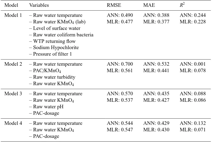
Table 2.Prediction models and goodness values of the models.

Model Variables RMSE MAE R2

Model 1 – Raw water temperature

– Raw water KMnO4(lab)

– Level of surface water – Raw water coliform bacteria – WTP returning flow – Sodium Hypochlorite – Pressure of filter 1

ANN: 0.490 MLR: 0.477

ANN: 0.388 MLR: 0.377

ANN: 0.244 MLR: 0.228

Model 2 – Raw water temperature

– PAC/KMnO4

– Raw water turbidity

– Raw water KMnO4

ANN: 0.700 MLR: 0.561

ANN: 0.532 MLR: 0.441

ANN: 0.001 MLR: 0.078

Model 3 – Raw water temperature

– Raw water KMnO4

– Raw water pH – PAC-dosage

ANN: 0.570 MLR: 0.537

ANN: 0.435 MLR: 0.427

ANN: 0.088 MLR: 0.086

Model 4 – Raw water temperature

– Raw water KMnO4

– PAC-dosage

ANN: 0.544 MLR: 0.547

ANN: 0.429 MLR: 0.430

ANN: 0.132 MLR: 0.071

The amount of residual aluminum is high when raw water

is cold even if the raw water KMnO4 and poly-aluminum

chloride (PAC) dosage are at the low level. When the raw

water temperature is higher and raw water KMnO4rises the

amount of residual aluminum is relatively low. This shows

the fact that the effectiveness of the water treatment process

is better when raw water is warmer which is very common in most of the WTP. It can be seen that autumn rains and

snow melting in the spring affects the quality of raw water

and the efficiency of the water treatment process. The raw

water color and KMnO4are at a higher level in the autumn,

late winter and spring seasons due to heavy raining and snow melting.

3.2 Prediction models

Prediction models were trained using 3/4 of the data and

tested using the final 1/4 of the data. Scaled and

interpo-lated dataset was used in modeling and the same variables were used in both MLR and ANN models. Created models

and calculated goodness of fit values (RMSE, MAE and R2₎

Figure 3.The testing periods of Model 1 (left) and the testing periods of Model 4 (right).

selected by a forward variable selection method. Model 2 was created using the best four variables of variable selec-tion presented in Juntunen et al. (2010) where the best MLP model was achieved with four variables. Manually selected variables were used in Model 3 and Model 4.

During the modeling session it was noticed that there are

several different combinations of variables that could be used

in modeling the residual aluminum with fairly good accu-racy. It was also noticed that the peak values of residual alu-minum could be predicted and the accuracy of the model improved only if some laboratory measurements of drink-ing water were used in the model. This, however, does not give any extra value for real-life application (EWS). The best prediction result was achieved with Model 1 and in Model 2 both ANN and MLR had the lowest accuracy of the

mod-els presented in this paper. The difference between ANN and

MLR is in Model 2 notably bigger than in Model 1. As it can be seen from Table 2, the error values of the ANN and MLR models were nearly the same in Models 1, 3 and 4, but ANN models seem to be slightly better in every variable set except in Model 2. The accuracy of MLR was better in Model 2 than the accuracy of ANN model. This is an opposite result than presented in Juntunen et al. (2010), where MLP showed a better performance than the MLR method. Modeling meth-ods were quite similar in both studies. Discrepancy between

the results could be explained by the significant differences

in data pre-processing. In Juntunen et al. (2010) the process data was averaged to 1 day data and combined with daily laboratory data, the measuring period was 275 days, and the

dataset was not scaled to range [−2...+2] using the new

non-linear scaling method.

The results of Model 1 and Model 4 testing periods are shown in Fig. 3 for both ANN and MLR methods. The baseline of the residual aluminum prediction is fairly good with both models. Modeled residual aluminum follows the changes of measured residual aluminum but the peak values could not be predicted. As the calculated results in Table 2

showed, the difference between ANN and MLR models is

minor. Model 4 was created using only three variables and the error values were not higher than in Model 1. This is an encouraging result for creating the EWS or on-line control. Almost the same accuracy can be attained with fewer vari-ables.

4 Conclusions

The purpose of this work was to analyze the data of the water

treatment plant, find out which variables affect the amount of

residual aluminum in drinking water, create as simple and reliable prediction models for residual aluminum as possible using ANN and MLR methods and to compare the accuracy of models with each other and to earlier presented results. Same modeling methods and the same data source were used

to study the effect of data pre-processing to modeling

accu-racy. Clear correlations to residual aluminum were found af-ter the dataset was scaled using the new nonlinear scaling method based on generalized norms and skewness. Variables that had the highest correlation to the amount of residual alu-minum were among others: the raw water temperature, raw

water KMnO4and PAC/KMnO4-ratio.

Decent prediction models were created using only a few important variables. The baseline of residual aluminum in drinking water can be predicted with fairly good accuracy with both MLR and ANN models. MLR and ANN methods gave almost the same results. Comparison to earlier results of modeling the residual aluminum at the same water treat-ment plant was done. In the earlier study the overall model-ing accuracy was slightly better. However, in this study the MLR method was found to be better than the ANN method when using the same variables as in the earlier study.

Dis-crepancy between the results can be explained by different

kind of data pre-processing. The accuracy of created

predic-tion models could be improved by using different variable

Edited by: L. Rietveld

References

Areerachakul, S. and Sanguansintukul, S.: A Comparison between the Multiple Linear Regression Model and Neural Networks for Biochemical Oxygen Demand Estimations, SNLP ’09, Eighth International Symposium on Natural Language Processing, 11– 14, 2009.

Audone, B. and Giunta, G.: Multiple Linear Regression to Detect

Shielding Effectiveness Degradations. International Symposium

on Electromagnetic Compatibility – EMC EUROPE 2008, 8–12 September 2008, 1–6, 2008.

Baxter, C. W., Stanley, S. J., and Zhang, Q.: Development of a full-scale artificial neural network model for the removal of natural organic matter by enhanced coagulation, J. Water Supply Res. T., 48, 129–136, 1999.

Baxter, C. W., Zhang, Q., Stanley, S. J., Shariff, R., Tupas, R.-R. T.,

and Stark, H. L.: Drinking water quality and treatment: the use of artificial neural networks, Can. J. Civil Eng., 28 (Suppl. 1), 26–35, 2001.

Beale, M. H., Hagan, M. T., and Demuth, H. B.: Neural Network Toolbox TM 7 User’s Guide, Matlab MathWorks Inc., September 2010.

Bowden, G. J., Nixon, J. B., Dandy, G. C., Maier, H. R., and Holmes, M.: Forecasting chlorine residuals in a water distribu-tion system using a general regression neural network, Math. Comput. Model., 44, 469–484, 2006.

Dayhoff, J. E.: Neural Network Architectures: An introduction, Van

Nostrand Reinhold, New York, ISBN: 0-442-20744-1, 259 pp., 1990.

Delgrange, N., Cabassud, C., Cabassud, M., Durand-Bourlier, L., and Laine, J. M.: Neural networks for prediction of ultrafiltration transmembrane pressure – application to drinking water produc-tion, J. Membrane Sci., 150, 111–123, 1998.

Delgrange-Vincent, N., Cabassud, C., Cabassud, M., Durand-Bourlier, L., and Laine, J. M.: Neural networks for long term

prediction of fouling and backwash efficiency in ultrafiltration

for drinking water production, Desalination, 131, 353–362, 2000. D’Errico, J.: “inpaint nans-function”, Matlab Central, File

Ex-chance, http://www.mathworks.com/matlabcentral/fileexchange/

4551 (last access: 26 October 2011), February 2004.

Driscoll, C. and Letterman, R.: Factors regulating residual alu-minium concentrations in treated water, Environmetrics, 6, 287– 309, 1995.

FINLEX: Decree of the Ministry of Social Affairs and Health:

Relating to the quality and monitoring of water intended for

Juntunen, P., Liukkonen, M., Pelo, M., Lehtola, M., and Hiltunen, Y.: Modelling of residual aluminum in water treatment process, in: Proceedings of the 7th EUROSIM Congress on Modelling and Simulation, 6–10 September 2010, Prague, Czech Republic, Vol. 2: Full Papers, 5 pp., 2010.

Juuso, E. K.: Data-based development of dynamic models for biological wastewater treatment in pulp and paper industry, Preprints of the 51st Conference on Simulation and Modelling, 14–15 October 2010, Oulu, Finland, 1–9, 2010.

Juuso, E. K.: Intelligent Trend Indices in Detecting Changes of Op-erating Conditions, in: Proceedings of UKSim 13th International Conference on Modelling and Simulation – UKSim 2011, Cam-bridge, UK, 30 March–1 April 2011, 162–167, 2011.

Kulkarni, P. and Chellam, S.: Disinfection by-product formation following chlorination of drinking water: Artificial neural net-work models and changes in speciation with treatment, Sci. Total Environ., 408, 4202–4210, 2010.

Leakey, H.: Aluminium residual management in drinking water us-ing selection criteria of aluminium based primary coagulants, M.Sc thesis, Royal Roads University Victoria, ISBN: 0-494-05113-2, 2004.

Maier, H. R., Morgan, N., and Chow, C. W. K.: Use of artificial neural networks for predicting optimal alum doses and treated water quality parameters, Environ. Modell. Softw., 19, 485–494, 2004.

Matlab Statistics Toolbox™ 7 User’s Guide, Matlab MathWorks

Inc., April 2011.

McLachlan, D. R. C., Bergeron, C., Smith, J. E., Boomer, D., and Rifat, S. L.: Risk for neuropathologically confirmed Alzheimer’s disease and residual aluminum in municipal drinking water em-ploying weighted residential histories, Neurology, 46, 401–405, 1996.

Pal, S. K. and Mitra, S.: Multilayer perceptron, fuzzy sets and clas-sification, IEEE Transactions on neural networks, 3, 683–697, 1992.

Shetty, G. R., Malki, H., and Chellam, S.: Predicting contaminant removal during municipal drinking water nanofiltration using ar-tificial neural networks, J. Membrane Sci., 212, 99–112, 2003. Tranmer, M. and Elliot, M.: Multiple Linear Regression, Catie

Marsh Centre for Census and Survey Research, Teaching papers, 47 pp., 2008.

WHO – World Health Organization: Aluminium in Drinking-water: Background document for development of WHO Guidelines for Drinking-water Quality, 2003.