https://doi.org/10.5194/se-8-987-2017
© Author(s) 2017. This work is distributed under the Creative Commons Attribution 3.0 License.
Methods and uncertainty estimations of 3-D structural modelling in
crystalline rocks: a case study
Raphael Schneeberger1, Miguel de La Varga2, Daniel Egli1, Alfons Berger1, Florian Kober3, Florian Wellmann2, and Marco Herwegh1
1Institute of Geological Sciences, University of Bern, Baltzerstrasse 1 + 3, 3012 Bern, Switzerland 2Graduate School AICES, RWTH Aachen University, Schinkelstrasse 2, 52062 Aachen, Germany 3Nagra, Hardstrasse 73, 5430 Wettingen, Switzerland
Correspondence to:Raphael Schneeberger ([email protected]) Received: 9 May 2017 – Discussion started: 12 May 2017
Revised: 16 August 2017 – Accepted: 21 August 2017 – Published: 28 September 2017
Abstract. Exhumed basement rocks are often dissected by faults, the latter controlling physical parameters such as rock strength, porosity, or permeability. Knowledge on the three-dimensional (3-D) geometry of the fault pattern and its con-tinuation with depth is therefore of paramount importance for applied geology projects (e.g. tunnelling, nuclear waste dis-posal) in crystalline bedrock. The central Aar massif (Cen-tral Switzerland) serves as a study area where we investi-gate the 3-D geometry of the Alpine fault pattern by means of both surface (fieldwork and remote sensing) and under-ground under-ground (mapping of the Grimsel Test Site) informa-tion. The fault zone pattern consists of planar steep major faults (kilometre scale) interconnected with secondary re-lay faults (hectometre scale). Starting with surface data, we present a workflow for structural 3-D modelling of the pri-mary faults based on a comparison of three extrapolation approaches based on (a) field data, (b) Delaunay triangula-tion, and (c) a best-fitting moment of inertia analysis. The quality of these surface-data-based 3-D models is then tested with respect to the fit of the predictions with the underground appearance of faults. All three extrapolation approaches re-sult in a close fit (>10 %) when compared with underground rock laboratory mapping. Subsequently, we performed a sta-tistical interpolation based on Bayesian inference in order to validate and further constrain the uncertainty of the extrapo-lation approaches. This comparison indicates that fieldwork at the surface is key for accurately constraining the geome-try of the fault pattern and enabling a proper extrapolation of major faults towards depth. Considerable uncertainties, how-ever, persist with respect to smaller-sized secondary
struc-tures because of their limited spatial extensions and unknown reoccurrence intervals.
1 Introduction
Geological information is inherently three-dimensional (3-D) in space but often represented in 2-D (Jones et al., 2009). With increasingly available computer power, 3-D modelling or geometrical visualizations have become widespread, as they can be performed on a desktop computer (e.g. Bistac-chi et al., 2008; Caumon et al., 2009; Hassen et al., 2016; Sausse et al., 2010; Stephens et al., 2015). 3-D models widely serve as a basis for subsequent investigations, such as stress modelling or fluid flow modelling (e.g. Hassen et al., 2016; Stephens et al., 2015). Explicit structural modelling can fur-ther be subdivided into stochastic and deterministic methods. Deterministic approaches yield a single output for input pa-rameters, analogous to drawing a map (e.g. Stephens et al., 2015), whereas as in stochastic approaches parameters are defined by a probabilistic density function with a component of randomness (e.g. Cherpeau and Caumon, 2015; González-Garcia and Jessell, 2016; Jørgensen et al., 2015; Koike et al., 2015).
tunnels or boreholes. Known information is then extrapolated towards the unknown. At the time of extrapolation, the valid-ity cannot be proven unless additional information, such as geophysical, borehole, or excavation data, is integrated.
Previous studies report that this extrapolation represents a main uncertainty within 3-D structural modelling of known structures (e.g. Baumberger, 2015; Bistacchi et al., 2008). From environments with sparse data, for example, the topol-ogy of the fault network is known to be highly uncertain or prone to the existence of unknown faults (e.g. Cherpeau et al., 2012; Cherpeau and Caumon, 2015; Hollund et al., 2002).
More generally, for kilometre-scale models, uncertainties in accuracy related to input data (i.e. GPS location, dip–dip azimuth measurements) are small compared to the uncer-tainty related to the data interpolation between known loca-tions or data extrapolation (Bond, 2015).
Uncertainties play an important role when considering decision-making based on information available from a 3-D model and have therefore been subject to extensive studies in the past (e.g. Bistacchi et al., 2008; Bond et al., 2007a; Lind-say et al., 2012; Tacher et al., 2006; Wellmann et al., 2010, 2014; Wellmann and Regenauer-Lieb, 2012; Yamamoto et al., 2014). Since models are a function of the data used, some of the approaches tend to analyse uncertainties in the input data before modelling (e.g. Bond et al., 2007b; Jones et al., 2009). Other approaches investigate the error propaga-tion into the models, inferring the uncertainty after modelling (Jessell et al., 2010; Lindsay et al., 2012; Viard et al., 2011; Wellmann et al., 2010). Most of these published studies were performed within sedimentary environments where parame-ters such as stratigraphy, layer thickness, layer orientation, and structural setting are well constrained. Uncertainty esti-mation and its potential reduction are less well constrained for the structural modelling of basement rocks (e.g. Svensk Kärnbränslehantering AB, 2009), which are characterized by intrusive contacts and a complex arrangement of deformation structures.
In this study, we focus on deformed basement rocks and the extrapolation of faults to depth. We follow two main goals: (i) the application of an extrapolation workflow for three different techniques for projection of surface structures to depth considering associated projection uncertainties and (ii) the design and application of a probabilistic approach to compare different extrapolation techniques in order to vali-date the generated models.
We focus specifically on the combination of observations in outcrops at the surface with observations in an under-ground facility, allowing for an extrapolation modelling ap-proach, and propose that it is possible to link these two types of observations in a probabilistic context by taking into ac-count uncertainties in measurements and the exact tie be-tween observed features at the surface and in the under-ground facility. We investigate a local case study in a rela-tively simple setting in crystalline rocks. The study area is characterized by well-exposed crystalline rocks of the Aar
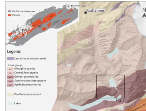
Figure 1.Geological map of the study area (modified after Berger et al., 2017). The coordinate system of the inset map is given in WGS84, whereas the coordinates of the local geological map are given in the Swiss coordinate system (CH1903).
massif in the central Swiss Alps (Fig. 1) and furthermore greatly benefits from subsurface information from the Grim-sel Test Site (GTS) underground rock laboratory run by the Swiss Cooperative for Disposal of Radioactive Waste (Na-gra).
This combination of good outcrop conditions at the sur-face and independent high-quality subsursur-face information al-lows for an extrapolation modelling approach and subsequent validation in a relatively simple and well-constrained high-topography crystalline setting.
2 Geological setting
The study site is located in the Haslital in the Central Alps (Switzerland; Fig. 1) within the Aar massif, an external crys-talline massif in the Alps representing exhumed basement rocks of the former European continental margin and thus belonging to the palaeogeographic Helvetic domain of the Alps (e.g. Mercolli and Oberhänsli, 1988; Pfiffner, 2009; von Raumer et al., 2009).
(Schneeberger et al., 2016). Furthermore, the concordant zir-con and titanite U–Pb intrusion ages of both rock units are overlapping within error; the GrGr intrusion has a concor-dant titanite U–Pb intrusion age of 299±2 Ma and the CAGr has an age of 299±2 Ma (Schaltegger and Corfu, 1992). The granitoids intruded during late to post-Variscan exten-sional tectonics into a polymetamorphic pre-Variscan base-ment (Abrecht, 1994; Berger et al., 2017; Labhart, 1977; von Raumer et al., 2009; Schaltegger, 1990, 1994).
Meta-basic dykes, formerly called lamprophyres (Ober-hänsli, 1986), intrude into the granitoid bedrock without al-tering the granitoid, indicating only slightly younger intru-sion ages of former basic dykes with respect to the calc-alkaline granitoids.
The aforementioned rock types are subsequently over-printed by metamorphism and deformation related to Alpine orogeny. Peak metamorphic conditions reached 450±30◦C
and 6±1 kbar (Challandes et al., 2008) at 22–20 Ma (Chal-landes et al., 2008; Rolland et al., 2009).
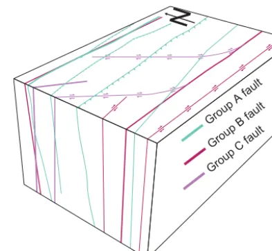
Several authors have described the deformation related to Alpine orogeny in the vicinity of the study area (e.g. Baum-berger, 2015; Challandes et al., 2008; Choukroune and Gapais, 1983; Goncalves et al., 2012; Keusen et al., 1989; Marquer et al., 1985; Rolland et al., 2009; Steck, 1968; Wehrens et al., 2016, 2017). Ductile deformation is ex-pressed by a pervasive foliation and localized high-strain zones (shear zones). The exact geometry of the 3-D shear zone network, which occurs at a variety of scales ranging from several kilometres down to millimetres, is complex (Choukroune and Gapais, 1983). It is, however, possible to extract a pattern of kilometre-long major shear zones inter-connected by hectometre-long subordinate bridging struc-tures. The major shear zones tend to be quasi-planar (Baum-berger, 2015; Wehrens et al., 2017) and we therefore as-sume a considerably simplified shear zone pattern with quasi-planar to quasi-planar geometries of the major shear zones grouped according to their strike orientation (Fig. 2).
The kinematic framework of Alpine deformation is con-troversial. Several kinematic models have been proposed for the shear zone network genesis in the study area, includ-ing sinclud-ingle-phase (Choukroune and Gapais, 1983) and multi-stage evolution models (Herwegh et al., 2017; Rolland et al., 2009; Steck, 1968; Wehrens et al., 2016, 2017). This study aims to reconstruct the present day 3-D geometry. Although the kinematic evolution is beyond the scope of this study, the generated models have been validated for kinematic in-consistency with respect to the known tectonic framework (e.g. models with unrealistic dip values have been removed; dip<60◦or north verging). The different orientations of the structures are therefore used without kinematic implications. The major orientation of structures within the area are NE– SW (group A), E–W (group B), and NW–SE (group C) trend-ing (Schneeberger et al., 2016; Wehrens et al., 2017).
The pervasive foliation and the highly localized shear zones form mechanical anisotropies, which favour
subse-N
Grou p A fa
ult
Grou p B fa
ult
Grou p C fa
ult
Figure 2.Schematic bloc diagram showing geometrical relation-ships between faults of different orientation groups (modified after Wehrens et al., 2017).
quent brittle localization (Belgrano et al., 2016; Kralik et al., 1992). Deformation in the brittle regime is expressed by frac-turing and cataclasis, often resulting in fault gouges (Bense et al., 2014; Wehrens et al., 2016). The spatial distribution of fractures and their reactivation in the form of fault gouge development is heterogeneous (Bossart and Mazurek, 1991; Mazurek, 2000).
Although the shear zones experienced a severe ductile de-formation history, most of them were reactivated in a brittle manner during the exhumation history (Wehrens et al., 2017). Subsequently, we therefore use the term fault as a summary term for high T ductile shear zones, low T ductile shear zones, and their reactivation by brittle shearing leading to cohesive (protocataclasite, cataclasite) or non-cohesive (fault gouge) fault rocks.
Present day seismic activity (Pfiffner and Deichmann, 2014) indicates ongoing recent tectonic activity in the deep subsurface of the Aar massif.
Glaciation and glacial retreat contributed to the latest his-tory of the area (Wirsig et al., 2016). Basal erosion and the latest young (17.7 ka, Wirsig et al., 2016) retreat ages produced excellent outcrop conditions, as most outcrops are glacially polished and above the treeline, exposing bare bedrock.
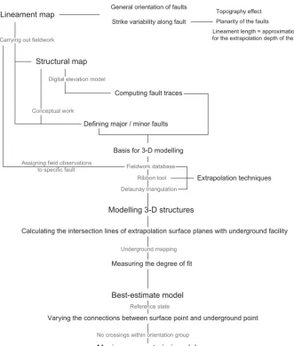
Extrapolation techniques
Lineament map General orientation of faults Strike variability along fault
Topography effect Planarity of the faults Lineament length = approximation for the extrapolation depth of the faults
Digital elevation model
Computing fault traces
Defining major / minor faults Carrying out fieldwork
Basis for 3-D modelling
Assigning field observations to specific fault
Ribbon tool
Delaunay triangulation Fieldwork database
Calculating the intersection lines of extrapolation surface planes with underground facility
Measuring the degree of fit Underground mapping
No crossings within orientation group Reference state
Varying the connections between surface point and underground point
Structural map
Modelling 3-D structures
Best-estimate model
Maximum a posteriori model Conceptual work
Figure 3.Employed modelling workflow to generate a 3-D structural model of the area based on a surface lineament map. As a major step, the workflow also considers the uncertainty related to the connection between mapped faults at the surface and underground.
3 Methods
3.1 Extrapolation workflow
In order to represent the 3-D geometry of faults, we devel-oped a workflow based on a combination of remote sensing and fieldwork (Fig. 3).
As a first step, we generated a lineament map using re-mote sensing data. We use the term lineament as defined by Gabrielsen and Braathen (2014) and O’Leary et al. (1976): a lineament is a mappable linear or curvilinear feature identi-fied by remote sensing, possibly representing the intersection between a planar to subplanar structural anisotropy and the Earth’s surface. Lineament mapping followed the method-ology presented by Baumberger (2015). Aerial photographs (swisstopo) and a digital elevation model (DEM; swisstopo) with resolutions of 0.5 and 2 m, respectively, served as a ba-sis.
Using the DEM, hillshade images (i.e. greyscale relief im-ages) with distinct illumination angles (0–360◦illumination azimuth with 45◦steps constant at a 30◦altitude angle) were calculated, resulting in eight hillshade images and illuminat-ing different parts of the investigation area. On a pixel-based map, the possible strike angle of a line depends on the num-ber of pixels of the raster matrix in which the line is enclosed (Heilbronner and Barrett, 2014). Our approach requires an angular resolution<10◦, and thus a minimum length of 10 pixels for a specific lineament was necessary to fulfil this criterion. Hence, shorter lineaments (<5 m) were discarded. Lineaments were manually digitized and are composed of a minimum of two endpoints and potentially several points in between.
in-dividual segments between a lineament’s nodes. In both ap-proaches, a weight is added to the strike proportional to the length of the lineament.
In addition to the aforementioned remote sensing ap-proach, conventional structural surface mapping over an area of 13 km2was performed. Spatially restricted outcrop obser-vations at the surface were extrapolated along strike using the lineament map; thus combining fieldwork and remote sens-ing allowed us to obtain a structural surface map. Ductile deformation was mapped by differentiating pervasive back-ground strain and localized high-strain zones (shear zones). At the surface, mapping of brittle deformation focused on the occurrence of fault gouges. In addition, mapping in the GTS underground facility was performed similarly to surface mapping on a decametre scale and in more detail regarding brittle structures (Schneeberger et al., 2016).
Structural modelling was performed using Move™ soft-ware (Midland Valley) on two distinct scales: a local scale (decametre) for the GTS and a regional scale (kilometre) for the entire study area. Underground 3-D structural mod-elling was performed on the basis of underground mapping and drill core data, which resulted in fault traces and ori-entations. This information provided the basis for the 3-D reconstruction of fault planes. Regional 3-D structural mod-elling was performed following published workflows using the surface fault map as a basis (e.g. Baumberger, 2015; Bis-tacchi et al., 2008; Kaufmann and Martin, 2009; Zanchi et al., 2009). Surface faults were extrapolated to depth by assigning a dip value to individual surface traces, where a trace is the intersection between the Earth’s surface and a fault. Three different extrapolation approaches were applied: (i) extrapo-lation along measured dip and dip azimuth (fieldwork-based approach). Data from outcrops were considered within an or-thogonal distance of <20 m to inferred fault traces and a strike differing less than 20◦ compared to the fault’s mean strike as defined by remote sensing. The fault’s mean strike was calculated via linear regression through all points defin-ing its trace. (ii) Delaunay triangulation is a meshdefin-ing algo-rithm that produces a triangulation for several points such that for a given point cloud, no point of the point cloud is in-side the circumcircle of any triangle connecting three points of the point cloud (Delaunay, 1934). It results in a 3-D sur-face interpolating the selected points. Based on this sursur-face, the entire fault trace can be extrapolated. Noise can arise be-cause of rugosities of the fault planes, uncertainties in tracing the fault intersection at the surface, and too-low vertical vari-ations in topography. In the case of near planar faults, the noise is reduced in the case of high variations in altitude be-tween valleys and mountain peaks and by preferring projec-tions of long fault traces over those of short fault segments. (iii) The ribbon tool is a Move™internal interpolation algo-rithm based on a three-points approach in which three points form a triangle and the orientation is averaged over a de-fined number of triangles (Midland Valley). The maximum dip orientation of each average triangle is represented as a
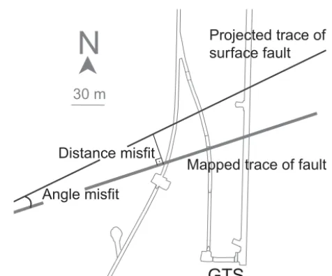
Angle misfit Distance misfit
Mapped trace of fault Projected trace of surface fault
30 m
N
GTS
Figure 4.Schematic drawing of hypothetical example for validation of 3-D models based on angular and distance misfit (map view). The contours of the GTS are shown in grey with a mapped fault trace and a fault trace resulting from projection of the fault plane from the surface.
stick at the location of the starting point. The combination of all sticks along a trace results in a plane for the given trace. More details on the method used by the ribbon tool are given in Fernandez (2005) and Baumberger (2015).
For each approach, the surface fault trace was extrap-olated to depth using the obtained specific orientation. Subsequently, the intersection line between the extrapo-lated plane and a horizontal plane at GTS elevation (ap-prox. 1730 m a.s.l.) was calculated. Then, the resulting inter-section lines were compared with the underground structural map in order to find the “best-fitting” underground structure to the obtained intersection line. The degree of fit between the intersection line at the surface and the trace of the under-ground structure was estimated using the orthogonal distance (distance misfit) starting from the intersection with the main gallery and the angular difference (angle misfit) between the two linear features (Fig. 4). Only structures within the same orientation group (groups A, B, C) were compared.
Furthermore, the degree of fit was compared between the different extrapolation approaches and thus for every surface fault. Considering all approaches, a best-fitting underground fault was assigned based on the aforementioned criteria. This assignment served as basis for the following structural mod-elling step in which every surface fault was linearly interpo-lated with the assigned best-fitting underground fault, yield-ing a “best-estimate” model.
3.2 Bayesian inference
above, we performed a Bayesian inference on the basis of a GTS parallel cross section. Bayes’ theorem,
p(θ|y)=p(θ )p(y|θ )
p(y) ,
provides a formal way to update probability distributions for model parametersθwhen new datay are obtained. The final goal is to obtain the posterior distribution p(θ|y) of the parametersθ given the observationsy. This distribution is proportional to the distribution of prior parameters p(θ )
and likelihood functionsp(y|θ ), which determine how likely these parameters are given specific observationsy. The term
p(y) is a normalization constant commonly referred to as evidence or marginal likelihood (see for example MacKay, 2003, for more details).
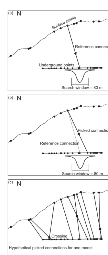
In this study scenario, we assign a parameter to each sur-face fault at the tunnel level. We represented the uncertainty about the exact value with a Gaussian distribution and a con-stant standard deviation of 40 m in the horizontal axis (Fig. 5) based on the dip uncertainty of 10◦ based on the dip vari-ation in multiple orientvari-ation measurements along a single fault (Fig. 5). As a mean value, we assign the best-estimate model from the previous interpolation. Interpolated planes were grouped according to their orientation into three sepa-rate groups (identified by A, B, C in the following; Fig. 2).
Within each orientation group, we expect faults to be mostly parallel with limited intersections based on field ob-servations. To capture this idea, we assigned a penalty fac-tor that reduces the log-likelihood of a parameter set for an increasing number of intersections (by 0.05 per intersec-tion, to be precise). The number of intersections per iteration was calculated using the Bentley–Ottmann algorithm (Sup-plement; Balaban, 1995; Bentley and Ottmann, 1979).
The described Bayesian inference cannot be performed di-rectly due to the complexity of multiple parameters in sev-eral groups and the non-linearities due to the fault intersec-tions. We therefore apply a computational sampling method based on an adaptive Metropolis MCMC approach (Haario et al., 2001) implemented in the probabilistic programming package PyMC 2 (Patil et al., 2010) and previously success-fully used in a geological context (de la Varga and Wellmann, 2016).
Final posteriors were discretized to match the locations of measured faults in the underground tunnel by a simple near-est location classifier (Fig. 5). Therefore, the final result of the inference is a discretized distribution of each of the pa-rameters. In order to compare the 3-D models obtained by the three extrapolations approaches, we then use the maxi-mum a posteriori value, i.e. the highest probability value of the posterior distributions.
N S
N S
N S
Surfac
e points
Underground points (a)
(b)
(c)
Search window = 80 m
Search window = 80 m Reference connection
Picked connection Reference connection
Hypothetical picked connections for one model Crossing
Figure 6. (a)Lineament map of the study area with underground rock laboratory. Topography contours are based on swissALTI3D (re-produced by permission from swisstopo; BA17063).(b)–(d)Length-weighted rose diagrams showing the endpoint-to-endpoint strike of all lineaments(b), lineaments longer than 400 m(c), and lineaments shorter than 400 m(d).(e)Length-weighted rose diagram showing the orientation of each segment of all lineaments.
4 Results
4.1 Lineament map
In total, 5277 lineaments with a spatially heterogeneous dis-tribution and lengths ranging from 5 to 1941 m were mapped (Fig. 6a). Lineaments are generally more concentrated along topographic highs and lows. Within certain areas (areas i and ii in Fig. 6a), the lineament’s strike tends to be parallel to the dip azimuth of the slopes, yielding uniform orienta-tions. In contrast, in domains with relatively low topographic variations, a variety of strike orientations become discernible (area iii in Fig. 6a).
Looking at the bulk data, lineaments show a major NE– SW and a minor NW–SE trend (Fig. 6b). Long lineaments (>
400 m) are mainly oriented NE–SW (Fig. 6c), whereas short lineaments show a considerable variation in strike (Fig. 6d). The two methods for estimating lineament orientations, end-point to endend-point (Fig. 6b) and individual segments (Fig. 6e), yield similar results.
4.2 Field observations and data
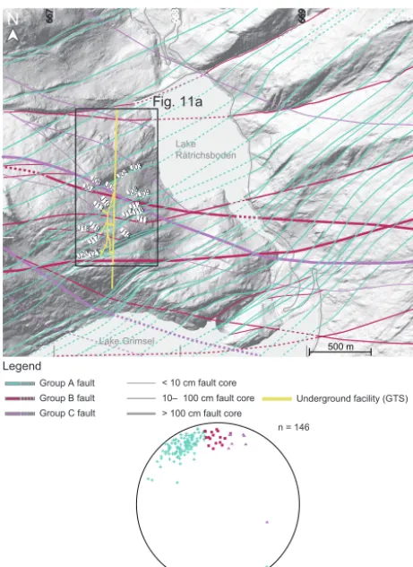
Data obtained from fieldwork combined with a compilation of several published maps (Baumberger, 2015; Keusen et al., 1989; Vouillomaz, 2009; Wehrens et al., 2017; Wicki, 2011) yielded a surface fault map (Fig. 7, see also Schnee-berger et al., 2016). Based on their orientation, we discrimi-nated different groups of faults (Fig. 7): group A are mainly steep SE-dipping faults. Their average orientation (dip az-imuth to dip) is 149/74. Group A faults mostly show steeply plunging stretching lineations resulting from ductile shear-ing. Group A can be correlated with faults formed during the Handegg phase (22–17 Ma) as defined by Wehrens et
al. (2017), while group B and group C would correspond to faults formed during the Oberaar phase (14–12 Ma; Wehrens et al., 2017). Group B are mainly steep S-dipping (mean orientation: 178/72) faults. Lastly, group C are SW-dipping faults coeval with group B with an average orientation of 196/72. Group C faults are subparallel to meta-basic dykes and often co-occur spatially with the latter. Groups B and C mostly show oblique to horizontal stretching lineations. For multiple orientation measurements along individual faults, the standard deviation of the mean dip azimuth was be-low 15◦and the mean dip below 10◦. Generally, the GrGr-dominated southern area shows an increased number of faults (Figs. 7 and 8). Detailed underground mapping resulted in a lithological (Fig. 8a) and a structural map of the GTS (Fig. 8b).
Meta-basic dykes occur as three distinct swarms, two lo-cated within the CAGr domain (Fig. 8a). The northern two swarms strike NW–SE, whereas the southern swarm strikes E–W; however, it is less clearly marked. Numerous dykes are overprinted by an Alpine foliation, which is sometimes oblique to the dyke boundary. Furthermore, dykes are often overprinted by localized ductile and brittle deformation ex-pressed by shear zones and fault gouges.
Faults occur along three NE–SW trending swarms, two E– W trending swarms, and two NW–SE trending swarms, lead-ing to a heterogeneous strain distribution along the under-ground facility (Fig. 8b).
Lake Grimsel Lake Rätrichsboden
< 10 cm fault core 10– 100 cm fault core > 100 cm fault core Group A fault
Legend
Group B fault Group C fault
Underground facility (GTS) J03
J12
J07J06J05J04
J08J09 J10
J11 J13
J14 J15
J20J21 J17
J16
J18J19
n = 146
500 m
670
160
161
668
667 669
N
Fig. 11a
Figure 7. Surface fault map with faults grouped by strike orien-tation (group A, B, C). Hillshade image underlying the map is based on swissALTI3D (reproduced by permission from swisstopo; BA17063). Fault exposure lines are dashed over uncertain areas and labelled in cases for which a connection to GTS exists. Lower hemi-sphere equal area projection with plane poles grouped according to strike. The map is based on the Swiss coordinate system.
The E–W trending swarms correspond to faults with orien-tations that are similar to group B. In total, 12 of these E–W striking faults were mapped.
The NW–SE trending fault swarms are localized mainly along dykes (Fig. 8) and represent group C structures. In to-tal, 25 NW–SE striking faults occur within the GTS.
Faults in the CAGr (northern part) seem to preferen-tially localize along pre-existing anisotropies, i.e. high-temperature brittle fractures (biotite coating) or meta-basic dykes, and thus form discrete faults (centimetre sized) with marked contacts to the host rock. In contrast, faults in the GrGr-dominated southern part form strain gradients over larger distances (metres). This observation is in agreement with the findings of Wehrens et al. (2017).
4.3 3-D structural modelling
The GTS model size is 600×250×100 m, whereas the re-gional model size was 4×3 km with a projection depth
reach-Legend
< 10 cm fault 10– 100 cm fault > 100 cm fault
30 m N Central Aare granite (CAGr) Grimsel granodiorite (GrGr)
Group A fault
Group B fault Group C fault Group A fault expected Legend
Central Aare granite (CAGr) Grimsel granodiorite (GrGr)
Meta-basic dyke (interpreted) Meta-basic dyke (mapped)
30 m N
(b) (a)
J03 J06
J07
J09
J08 J11
J12
J13
J14
J16
J20 J21
Fig. 11b
Figure 8. (a)Petrographic underground map.(b)Structural map-ping (1 : 1000) of the underground rock laboratory (GTS) with faults grouped according to their strike. Indicated labels correspond to sur-face fault labelling and represent the maximum a posteriori interpo-lation.
ing the underground facility for all faults. The projection depth was defined arbitrarily but no larger than half of the fault trace’s length. All 3-D models are provided in the Sup-plement.
4.3.1 GTS model
geomet-rical considerations, we infer the occurrence of three ma-jor dykes from which all others either fan out or form relay structures between the major dykes. Based on the field obser-vation that the major faults and relay structures dip steeply sub-vertically towards the south, we discriminated 8 major group A faults and 23 relay structures. Major group A faults occur within each NE–SW trending swarm discriminated on the map view. Group B deformation structures can be further subdivided into six major and seven relay faults. Group C de-formation structures can be subdivided into 6 major and 32 relay deformation structures, some of which are very short (14 m).
4.3.2 Regional model
The surface fault map (Fig. 7) served as a basis for the gener-ation of the three different kilometre-scale 3-D models (see above). All three modelling approaches yielded the 3-D ge-ometrical visualization of the surface fault pattern. They all share the same fault traces at the model surface. As men-tioned above, projection specific dip values were used for each of the models. However, not all surface faults were ex-trapolated with each approach. Of the 21 possible surface faults, 10 were extrapolated with the fieldwork-based ap-proach, 11 using the Delaunay triangulation, and 13 with the ribbon tool method. Missing projections can be due to a lack of outcrop description or the absence of sufficient to-pographic relief for remote-sensing-based approaches.
By combining all three approaches, at least 1 (but up to 3) degrees of fit with underground faults were calculated for each surface fault. Based on the different degrees of fit, a best-fitting underground structure was assigned to each sur-face fault. By linearly interpolating the two traces, we ob-tained a model which we called best-estimate model. In total, 11 group A faults reach the GTS. From the total 11, 7 have a dip<80◦, which would correspond to the major structures defined in the above-presented GTS-scale model, whereas the 4 steeper faults correspond to relay structures. Moreover, two group B and eight group C faults connect the surface with the GTS. The combination of all faults yields an av-erage spacing of 25.4 m, and faults appear to converge with depth.
4.3.3 Bayesian inference
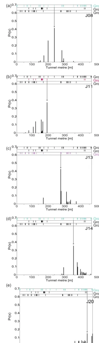
For each model that is obtained when each surface point (in-tersection between surface fault and 2-D section along the GTS) is interpolated with a specific underground point, the number of intersections was calculated and the likelihood of the model compiled based on the number of intersections. In total 10 000 models were calculated and for each a prob-ability for a certain interpolation of a specific surface point with an underground point was obtained (Fig. 9). For cer-tain surface points, a clear maximum a posteriori value was
0 0.2 0.3 0.4 0.5 0.6 0.7
Tunnel metre [m]
0 100 200 300 400 500
0.1
J20 Group A Group B Group C 0
0.2 0.3 0.4 0.5 0.6 0.7
Tunnel metre [m]
0 100 200 300 400 500
J14
0.1 0 0.2 0.3 0.4 0.5 0.6 0.7
Tunnel metre [m]
0 100 200 300 400 500
J13
0.1 0 0.2 0.3 0.4 0.5 0.6 0.7
Tunnel metre [m]
0 100 200 300 400 500
J11
0.1 0 0.2 0.3 0.4 0.5 0.6 0.7
Tunnel metre [m]
0 100 200 300 400 500
J08
0.1
Group A Group B Group C Group A Group B Group C
Pr(x)
Pr(x)
Pr(x)
(c) (b) (a)
Group A Group B
Group C
Group A Group B Group C
Pr(x)
Pr(x)
(d)
(e)
Figure 9.Probability distributions of five selected examples: panels
(a)to (d)show the highest probabilities achieved, whereas panel
J01J02 J03
J06 J07
J08 J09
J11J12J13
J14 J16 J20 J21
Group A Group B Group C
100 m
Underground lab.
Topography
N S
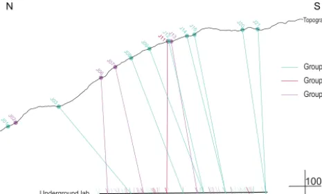
Figure 10. Cross section showing maximum a posteriori connec-tions between surface and underground faults. Faults are grouped and coloured according to their strike. Underground faults are rep-resented by short ticks; the less transparent ones have a connection to the surface.
found (Fig. 9a–d); however, for other surface points no un-derground point could be assigned unambiguously (Fig. 9e). Based on the maximum a posteriori value, a 3-D structural model was obtained by linearly interpolating each surface point to the underground point with the maximum a poste-riori value. We call this model the “maximum a posteposte-riori” model (Fig. 10). Note that the maximum a posteriori model only adds information to the initial model through considera-tion of a likelihood, i.e. the assumpconsidera-tion that crossing faults at a large scale are unlikely. Note that the smaller-scaled relay structures are not considered in this approach.
This maximum a posteriori interpolation model served as a basis for comparing different employed extrapolation ap-proaches. The comparison did not yield a clear “best” ex-trapolation approach; however, it seems that fieldwork-based approach results in the most accurate extrapolation.
5 Discussion 5.1 Lineament map
A comparison of the remote-sensing-based lineament map and field data showed that in intact granitic rocks, purely ductile shear zones without later brittle overprinting are not detected by remote sensing. Brittle deformation generating fractures, cataclasites, or even fault gouges responsible for mechanical weakening is necessary to form morphologically detectable structures (Fig. 11a; Baumberger, 2015). More-over, the orientations of the slopes play an important role, as faults striking in the down-dip directions of slopes are prone to the most effective erosion processes driven by gravity. Dif-ferent orientations observed on the lineament map (Fig. 6a, areas i and ii) for the eastern and western flank of the Hasli valley are interpreted to result from such preferential erosion. In contrast, the surface area (iii) in Fig. 6a is nearly
horizon-(b) (a)
S N S N
Granite
Meta-basic dyke SZ FG
20 cm
Figure 11. (a)Mountainside with incisions and exfoliation joints.
(b)Detailed picture of underground outcrop showing outcrop con-ditions and key structural features: a ductile shear zone (SZ) and a fault gouge (FG).
tal, thus reflecting a homogeneously eroded pattern of inter-section for lineaments. The dependence on erosion for the formation of morphological incisions leads to the observed heterogeneous lineament density distribution as ridges and valleys show higher lineament densities.
Endpoint-to-endpoint strike and the strikes of individual segments of lineaments are very similar (Fig. 6b and e), indicating only small variation in the strike of the linea-ments themselves. Therefore, underlying structures should be quasilinear to linear in 2-D and planar in 3-D. We also observe that the longest lineaments are NE–SW striking and that the variability shown in Fig. 6e is mostly due to vary-ing strike orientations of very short lineaments (<20 m). In addition to the NE-SW striking maximum, few long linea-ments strike NW–SE. Both major orientations are similar to those reported from field observations (Figs. 7 and 8) and correlate with previous studies (Rolland et al., 2009; Steck, 1968; Wehrens et al., 2017), indicating that lineament maps are suitable to obtain the general trend of steep faults in well-exposed crystalline terrain. Much care is needed, however, when further interpreting lineament maps, as the geologic meaning of the lineament is ambiguous and lineament maps are strongly operator dependent (e.g. Scheiber et al., 2015).
5.2 Field observations and data
Differences between the surface map and the underground map are relatively small. The spacing of faults at the surface is lower, but general orientations are comparable (Figs. 7 and 8) and the two mappings are thus discussed jointly.
Localization processes seem to differ between the two host rocks (CAGr and GrGr; Wehrens et al., 2017). The higher amount of biotite in the GrGr could influence the rock’s rheology towards more ductile behaviour. In contrast, the relatively higher amount of quartz and K-feldspars renders the CAGr more brittle than GrGr at similar pressureP and temperature T conditions and thus enforces brittle fractur-ing and possible subsequent ductile shear zone widenfractur-ing, as observed in other crystalline rocks (Guermani and Pennac-chioni, 1998; Mancktelow and PennacPennac-chioni, 2005; Wehrens et al., 2016, 2017). Hence any mechanical anisotropy, such as along pre-existing structures in the form of magmatic shear zones, meta-basic dykes, or aplitic dykes, served in the CAGr as sites for strain localization when suitably oriented with re-spect to the stress field.
5.3 3-D structural modelling
Our 3-D structural models were generated as a contribution to a project monitoring several parameters, such as micro-seismicity and in situ stress conditions, on the kilometre scale (large-scale monitoring; Nagra). Therefore, 3-D structural models were required mostly for visualization purposes. A deterministic explicit modelling workflow was required, as often is used in applied projects. It is, however, clear that for model updating, an implicit modelling approach would re-sult in faster data handling. The deterministic approach was chosen because we attempted to obtain a geometrically sat-isfying product within the simplest geological setting pos-sible. Furthermore, we were interested in the actual geom-etry of the faults dissecting granitoid rock bodies. Lastly, the uncommonly well-constrained setting of our study site (high-resolution underground data) was used to test and po-tentially validate extrapolation techniques for common appli-cation. Therefore, the underground data were only integrated as validation and not as a constraint during interpolation.
5.3.1 Three different approaches to obtain extrapolation 3-D structural models (kilometre-scale models)
Uncertainty related to the assignment of specific dip val-ues to lineament traces (Baumberger, 2015; Bistacchi et al., 2008) led to the comparison of three different approaches. Validation attempts by comparison with underground map-ping are purely geometrical and were based on two criteria, namely angle and distance misfit (Fig. 4). All three extrap-olation approaches yielded similar results and no significant differences were observed. Moreover, in order to allow for a thorough comparison between the different extrapolation ap-proaches solely based on the angle and distance misfit, the underground faults would need to be homogeneously dis-tributed, which is not the case (Fig. 8).
The validation procedure could be refined using fault core thickness. However, fault thickness varies substantially along
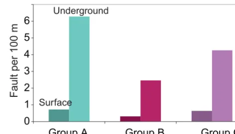
Group A Group B Group C
Underground
Fault per 100 m
0 1 2 3 4 5 6
Surface
Figure 12.Histogram showing the number of faults grouped per strike at the Earth’s surface and underground (GTS).
strike (e.g. Torabi and Berg, 2011) and thus is not a clear distinction criterion.
In addition to the average dip, the maximum and minimum dips could be used, which would yield a projection cone sim-ilar to the uncertainty visualization suggested by Baumberger (2015). Applying this approach to a restricted area, such as the underground rock laboratory investigated in this study, re-sulted in total coverage and no possible distinction between different faults. However, for a final representation of the un-certainty related to the dip value on a regional scale (kilome-tre scale), the approach of visualizing projection cones would suit.
5.3.2 GTS (decametre-scale model) compared with kilometre-scale “best-estimate” model
As a result of differences in outcrop conditions, the number of observed faults is significantly higher in the underground laboratory compared to the surface (Fig. 12). Underground, nearly 100 % of polished outcrop is accessible along the tun-nel walls (Fig. 11b), whereas at the surface faults are often covered with vegetation, even in relatively vegetation-poor domains.
Furthermore, we observe convergence of surface faults with depth in our best-estimate model, which could be a modelling artefact. The N–S extent of surface area is larger compared to the GTS area, leaving a northern and a southern surface part underneath for which no underground data ex-ist (Fig. 10). Hence faults in these domains are forced by the model set-up to be connected to the underground, leading to artificial fault orientations in these two cases (N and S rims of Fig. 13a). For that reason, only faults in the central part of the best-estimate model will be further considered.
5.3.3 “Maximum a posteriori” model
‘Maximum a posteriori’ Fieldwork Delaunay tri.
Group A faults
Ribbon tool
Underground lab.
Topography
N S
100 m (a)
(b)
‘Maximum a posteriori’ Fieldwork Delaunay tri.
Group B and C faults
Ribbon tool
Underground lab.
Topography
N S
100 m
Figure 13.Comparison of maximum a posteriori interpolation with three extrapolation approaches used to assign dip to fault exposure line. Figure subdivided into(a)group A (NE–SW),(b)group B (E– W), and group C (NW–SE). Group B and group C are displayed jointly as group B, which contains only two faults.
model was considered. Assuming no intersections within a large-scale fault set is simplistic, but from field observations it seems plausible (Fig. 7) as a first approach for faults be-longing to a specific orientation group (group A, B, C). The maximum a posteriori model is based on a N–S cross section along the GTS, and this orientation implies that faults would only cross if their dip varies strongly. Such a strong variation in the dip value is improbable based on measured dip values (Fig. 7). Therefore, this assumption seems feasible.
This simplistic representation of nature enabled us to ob-tain a probability for all possible interpolations between a specific surface point and all underground points of the cor-responding orientation group. As previously mentioned, the margins of the interpolation space show boundary artefacts, and thus the following surface points at the model margin were not further considered: J03, J06, J20, and J21 (Fig. 8). As expected, probability densities are skewed towards the area of lesser fault density (Fig. 9). At this point it is impor-tant to remember that probability density is given as area, and therefore we cannot directly compare the discretized posteri-ors since they are a function of the distance between nearby faults.
We compared the initial three extrapolation techniques based on the maximum a posteriori model (Fig. 13). When comparing group A faults, fieldwork-based extrapolation closely fit the maximum a posteriori interpolation, which in-dicates either that the fieldwork-based model yields the best results or validates the Bayesian inference approach depend-ing on whether the reference state is the statistical inter-polation or the measured field data. Generally, dips of the maximum a posteriori models are slightly steeper than mea-sured dips during fieldwork (Fig. 14a). However, the dip differences between the fieldwork-based extrapolation 3-D structural model and the maximum a posteriori interpola-tion model are small (Fig. 14b). Also, the dip differences between the ribbon-tool-based 3-D structural model and the maximum a posteriori interpolation model are small, but dips obtained via the ribbon tool are systematically steeper, which does not correspond to the measured dips (Fig. 14a). The ex-trapolation 3-D structural model obtained via Delaunay tri-angulation is less close to the maximum a posteriori interpo-lation model and obtained dips vary substantially.
The comparison for the group B and C faults is less clear. Fieldwork-based and ribbon tool extrapolations are close to the maximum a posteriori model (Fig. 13). Therefore, we conclude that fieldwork is still necessary for 3-D structural modelling in crystalline environments and that the ribbon tool (Move™) offers numerous options to tune the obtained plane; however, this tuning requires a profound conceptual background model.
5.3.4 Possible model refinements
Presented surface models include only major faults (Fig. 15). However, for further applications, such as groundwater flow modelling or slip tendency analysis, not only major faults are of interest but also their relay structures. Based on the orien-tation information gained from the regional kilometre-scale models and on the intersection pattern observed during linea-ment mapping, it is possible to infer a near surface 3-D model not only with the major fault but also the relay structure. Fur-thermore, the increased level of detail in the GTS model (de-cametre scale) forms a similar model in the underground. The unknown space between the two models would require prob-abilistic modelling with several key parameters, for example fault spacing, fault orientations, apertures, or cross-cutting relationships.
6 Conclusions
The exceptional opportunity for a surface and underground data comparison over 3-D structural modelling approaches led us to the following conclusions:
60 65 70 75 80 85 90
Fieldwork Delaunay MAP
Dip [°]
D
ip
d
iff
er
en
ce
v
s. M
A
P
[°
]
Fieldwork Delaunay Ribbon tool
0 5 10 15
(b) (a)
Ribbon tool
Figure 14. (a)Box plot showing dip value for different extrapolation approaches and for maximum a posteriori (MAP) interpolation.(b)Box plots for dip comparison between different extrapolation approaches and the maximum a posteriori (MAP) interpolation.
Figure 15.Representation in 3-D of the maximum a posteriori model of fault geometry with three different angles of view. N is indicated by the black triangle. The black tunnel is 717 m long.
Structural surface mapping allowed for a discrimination of three orientation groups of faults.
Comparison based on geometrical criteria (distance and angle misfit) of the three approaches to extrapolate to depth surface traces yielded comparable results for all extrapola-tion approaches.
Interpolation of surface data with underground data based on a Bayesian inference problem showed that the fieldwork-based approach is the most accurate extrapolation technique. However, this could also validate the interpolation approach. We conclude, similarly to Zanchi et al. (2009), that for 3-D structural modelling a high-topography area within crys-talline bedrock, classical fieldwork as an information source and as a basis for a conceptual background model on which interpolations or extrapolations performed within 3-D struc-tural modelling can be examined for validity. In terms of gen-eral fault networks, our approach can be applied to (i) perva-sive regional fault or fracture patterns. Currently it will fail in the case of (ii) discrete large-scale faults (e.g. strike-slip faults) consisting of one fault core and an associated damage zone. In such cases, more elaborate probabilistic models have to be generated in future, including 3-D variations in terms of spacing and orientation of secondary faults and splay faults. (i) Even with limited or missing underground information, our approach can be used to predict a surface-based 2-D model including a probability evaluation (e.g. variable dip
angles) with depth. If available, this evaluation can be tested with individual depth points such as drill core information. Additionally, an expansion towards 3-D would require prob-ability attributes for dip azimuths.
Data availability. The research data can be freely accessed. The 3-D models can be found in the supplementary material. All structural measurements are also enclosed within the models.
The Supplement related to this article is available online at https://doi.org/10.5194/se-8-987-2017-supplement.
Competing interests. The authors declare that they have no conflict of interest.
Edited by: Bernhard Grasemann
Reviewed by: Clare Bond, Gautier Laurent, and one anonymous referee
References
Abrecht, J.: Geologic units of the Aar massif and their pre-Alpine rock associations: a critical review, Schweizerische Mineral. und Petrogr. Mitteilungen, 74, 5–27, https://doi.org/10.5169/seals-56328, 1994.
Balaban, I. J.: An optimal algorithm for finding segments inter-sections, in: Proceedings of the eleventh annual symposium on Computational geometry – SCG ’95, pp. 211–219, ACM Press, New York, New York, USA, 1995.
Baumberger, R.: Quantification of lineaments: Link between inter-nal 3D structure and surface evolution of the Hasli valley (Aar massif, Central Alps, Switzerland), PhD thesis, University of Bern, Switzerland, 2015.
Belgrano, T. M., Herwegh, M., and Berger, A.: Inherited struc-tural controls on fault geometry, architecture and hydrothermal activity?: an example from Grimsel Pass, Switzerland, Swiss J. Geosci., 109, 345–364, https://doi.org/10.1007/s00015-016-0212-9, 2016.
Bense, F. A., Wemmer, K., Löbens, S., and Siegesmund, S.: Fault gouge analyses: K-Ar illite dating, clay mineralogy and tectonic significance – a study from the Sierras Pampeanas, Argentina, Int. J. Earth Sci., 103, 189–218, https://doi.org/10.1007/s00531-013-0956-7, 2014.
Bentley, J. L. and Ottmann, T. A.: Algorithms for Reporting and Counting Geometric Intersections, IEEE Trans. Comput., C-28, 643–47, https://doi.org/10.1109/TC.1979.1675432, 1979. Berger, A., Mercolli, I., Herwegh, M., and Gnos, E.: Explanatory
notes accompanying the geological map of the Aar massif and the Tavetsch- and Gotthard Nappes, Geological Special Map 129, Swisstopo, Wabern, Switzerland, 2017.
Bistacchi, A., Massironi, M., Dal Piaz, G. V., Dal Piaz, G., Mo-nopoli, B., Schiavo, A., and Toffolon, G.: 3D fold and fault reconstruction with an uncertainty model: An example from an Alpine tunnel case study, Comput. Geosci., 34, 351–372, https://doi.org/10.1016/j.cageo.2007.04.002, 2008.
Bond, C. E.: Uncertainty in structural interpretation: Lessons to be learnt, J. Struct. Geol., 74, 185–200, https://doi.org/10.1016/j.jsg.2015.03.003, 2015.
Bond, C. E., Gibbs, A. D., Shipton, Z. K., and Jones, S.: What do you think this is? “Conceptual uncertainty” In geoscience interpretation, GSA Today, 17, 4–10, https://doi.org/10.1130/GSAT01711A.1, 2007a.
Bond, C. E., Shipton, Z. K., Jones, R. R., Butler, R. W. H., and Gibbs, A. D.: Knowledge Transfer in a digital world: Field data acquisition, uncertainty and data management, Geosphere, 3, 568–576, https://doi.org/10.1130/GES00094.1, 2007b.
Bossart, P. and Mazurek, M.: Structural geology and water flow-paths in the migration shear-zone, Nagra technical report NTB 91-12, Wettingen, Switzerland, 1991.
Caumon, G., Collon-Drouaillet, P., Le Carlier de Veslud, C., Viseur, S., and Sausse, J.: Surface-Based 3D Model-ing of Geological Structures, Math. Geosci., 41, 927–945, https://doi.org/10.1007/s11004-009-9244-2, 2009.
Challandes, N., Marquer, D., and Villa, I. M.: P-T-t modelling, fluid circulation, and 39 Ar–40 Ar and Rb-Sr mica ages in the Aar Massif shear zones (Swiss Alps), Swiss J. Geosci., 101, 269– 288, https://doi.org/10.1007/s00015-008-1260-6, 2008. Cherpeau, N. and Caumon, G.: Stochastic structural
mod-elling in sparse data situations, Pet. Geosci., 21, 233–247, https://doi.org/10.1144/petgeo2013-030, 2015.
Cherpeau, N., Caumon, G., Caers, J., and Lévy, B.: Method for Stochastic Inverse Modeling of Fault Geometry and Con-nectivity Using Flow Data, Math. Geosci., 44, 147–168, https://doi.org/10.1007/s11004-012-9389-2, 2012.
Choukroune, P. and Gapais, D.: Strain pattern in the Aar Granite (Central Alps): orthogneiss developed by bulk inhomogeneous flattening, J. Struct. Geol., 5, 411–418, 1983.
Delaunay, B.: Sur la sphère vide. A la mémoire de Georges Voronoi, Bull. l’Académie des Sci. l’URSS. Cl. des Sci. mathématiques Nat., 6, 793–800, 1934.
de la Varga, M. and Wellmann, J. F.: Structural geologic modeling as an inference problem: A Bayesian perspective, Interpretation, 4, SM1–SM16, 2016.
Fernández, O.: Obtaining a best fitting plane through 3D georeferenced data, J. Struct. Geol., 27, 855–858, https://doi.org/10.1016/j.jsg.2004.12.004, 2005.
Gabrielsen, R. H. and Braathen, A.: Models of fracture linea-ments – Joint swarms, fracture corridors and faults in crystalline rocks, and their genetic relations, Tectonophysics, 628, 26–44, https://doi.org/10.1016/j.tecto.2014.04.022, 2014.
Goncalves, P., Oliot, E., Marquer, D., and Connolly, J. A. D.: Role of chemical processes on shear zone formation: an example from the Grimsel metagranodiorite (Aar massif, Central Alps), J. Metamorph. Geol., 30, 703–722, https://doi.org/10.1111/j.1525-1314.2012.00991.x, 2012.
González-Garcia, J. and Jessell, M.: A 3D geological model for the Ruiz-Tolima Volcanic Massif (Colombia): Assess-ment of geological uncertainty using a stochastic approach based on Bézier curve design, Tectonophysics, 687, 139–157, https://doi.org/10.1016/j.tecto.2016.09.011, 2016.
Guermani, A. and Pennacchioni, G.: Brittle precursors of plastic deformation in a granite: an example from the Mont Blanc massif (Helvetic, western Alps), J. Struct. Geol., 20, 135–148, 1998. Haario, H., Saksman, E., and Tamminen, J.: An adaptive metropolis
algorithm, Bernoulli, 7, 223–242, 2001.
Hassen, I., Gibson, H., Hamzaoui-Azaza, F., Negro, F., Rachid, K., and Bouhlila, R.: 3D geological modeling of the Kasser-ine Aquifer System, Central Tunisia: New insights into aquifer-geometry and interconnections for a better assess-ment of groundwater resources, J. Hydrol., 539, 223–236, https://doi.org/10.1016/j.jhydrol.2016.05.034, 2016.
Heilbronner, R. and Barrett, S.: Image Analysis in Earth Sciences, Springer, Berlin Heidelberg, 2014.
Herwegh, M., Berger, A., Baumberger, R., Wehrens, P., and Kissling, E.: Large-Scale Crustal-Block-Extrusion During Late Alpine Collision, Sci. Rep., 7, 413, https://doi.org/10.1038/s41598-017-00440-0, 2017.
Jessell, M. W., Aillères, L., and de Kemp, E. A.: To-wards an integrated inversion of geoscientific data: What price of geology?, Tectonophysics, 490, 294–306, https://doi.org/10.1016/j.tecto.2010.05.020, 2010.
Jones, R. R., McCaffrey, K. J. W., Clegg, P., Wilson, R. W., Holli-man, N. S., Holdsworth, R. E., Imber, J., and Waggott, S.: In-tegration of regional to outcrop digital data: 3D visualisation of multi-scale geological models, Comput. Geosci., 35, 4–18, https://doi.org/10.1016/j.cageo.2007.09.007, 2009.
Jørgensen, F., Høyer, A., Sandersen, P. B. E., and He, X.: Combining 3D geological modelling techniques to address variations in geology, data type and density – An exam-ple from Southern Denmark, Comput. Geosci., 81, 53–63, https://doi.org/10.1016/j.cageo.2015.04.010, 2015.
Kaufmann, O. and Martin, T.: 3D geological modelling from bore-holes, cross-sections and geological maps, application over for-mer natural gas storages in coal mines, Comput. Geosci., 35, 70– 82, https://doi.org/10.1016/S0098-3004(08)00227-6, 2009. Keusen, H. R., Ganguin, J., Schuler, P., and Buletti, M.: Felslabor
Grimsel: Geologie, Nagra technical report NTB 87-14, Baden, Switzerland, 1989.
Koike, K., Kubo, T., Liu, C., Masoud, A., Amano, K., Kurihara, A., Matsuoka, T., and Lanyon, B.: 3D geostatistical modeling of fracture system in a granitic massif to characterize hydraulic properties and fracture distribution, Tectonophysics, 660, 1–16, https://doi.org/10.1016/j.tecto.2015.06.008, 2015.
Kralik, M., Clauer, N., Holnsteiner, R., Huemer, H., and Kappel, F.: Recurrent fault activity in the Grimsel Test Site (GTS, Switzer-land): revealed by Rb-Sr, K-Ar and tritium isotope techniques, J. Geol. Soc. London., 149, 293–301, 1992.
Labhart, T.: Aarmassiv und Gotthardmassiv, Gebruder Borntraeger Verlagsbuchhandlung, Berlin and Stuttgart, 173 p., 1977. Lindsay, M. D., Aillères, L., Jessell, M. W., de Kemp, E. A.,
and Betts, P. G.: Locating and quantifying geological uncer-tainty in three-dimensional models: Analysis of the Gippsland Basin, southeastern Australia, Tectonophysics, 546–547, 10–27, https://doi.org/10.1016/j.tecto.2012.04.007, 2012.
MacKay, D. J. C.: Information Theory, Inference, and Learning Al-gorithms, 4th edition, Cambridge University Press, Cambridge, UK, 2003.
Mancktelow, N. S. and Pennacchioni, G.: The control of precursor brittle fracture and fluid–rock interaction on the development of single and paired ductile shear zones, J. Struct. Geol., 27, 645– 661, https://doi.org/10.1016/j.jsg.2004.12.001, 2005.
Marquer, D., Gapais, D., and Capdevila, R.: Chemical-changes and mylonitization of a granodiorite within low-grade metamorphism (Aar massif, central Alps), Bull. Mineral., 108, 209–221, 1985. Mazurek, M.: Geological and hydraulic properties of
water-conducting features in crystalline rocks, in: Hydrogeology of crystalline rocks, vol. 34, edited by: Stober, I. and Bucher, K., pp. 3–26, Springer, the Netherlands, 2000.
Mercolli, I. and Oberhänsli, R.: Variscan tectonic evolu-tion in the Central Alps: a working hypothesis, Schweiz-erische Mineral. und Petrogr. Mitteilungen, 68, 491–500, https://doi.org/10.5169/seals-52084, 1988.
Oberhänsli, R.: Geochemistry of meta-lamprophyres from the Cen-tral Swiss Alps, Schweizerische Mineral. und Petrogr. Mitteilun-gen, 66, 315–342, 1986.
O’Leary, D. W., Friedman, J. D., and Pohn, H. A.: Lineament, linear, lineation?: Some proposed new standards for old terms, Geol. Soc. Am. Bull., 87, 1463–1469, https://doi.org/10.1130/0016-7606(1976)87<1463:LLLSPN>2.0.CO;2, 1976.
Patil, A., Huard, D., and Fonnesbeck, C. J.: PyMC: Bayesian stochastic modelling in Python, J. Stat. Softw., 35, 1–81, 2010. Pfiffner, O. A.: Geologie der Alpen, Haupt Verlag, Bern, Stuttgart,
Wien, 2009.
Pfiffner, O. A. and Deichmann, N.: Seismotektonik der Zen-tralschweiz, Wettingen, Switzerland, 2014.
Rolland, Y., Cox, S. F., and Corsini, M.: Constraining deformation stages in brittle–ductile shear zones from combined field map-ping and 40Ar/39Ar dating: The structural evolution of the Grim-sel Pass area (Aar Massif, Swiss Alps), J. Struct. Geol., 31, 1377– 1394, https://doi.org/10.1016/j.jsg.2009.08.003, 2009.
Sausse, J., Dezayes, C., Dorbath, L., Genter, A., and Place, J.: 3D model of fracture zones at Soultz-sous-Forêts based on ge-ological data, image logs, induced microseismicity and verti-cal seismic profiles, Comptes Rendus-Geosci., 342, 531–545, https://doi.org/10.1016/j.crte.2010.01.011, 2010.
Schaltegger, U.: The Central Aar Granite: Highly differentiated calc-alkaline magmatism in the Aar massif (Central Alps, Switzerland), Eur. J. Mineral., 2, 245–259, 1990.
Schaltegger, U.: Unravelling the pre-Mesozoic history of Aar and Gotthard massifs (Central Alps) by isotopic dating: a review, Schweizerische Mineral. und Petrogr. Mitteilungen, 74, 41–51, https://doi.org/10.5169/seals-56330, 1994.
Schaltegger, U. and Corfu, F.: The age and source of late Hercynian magmatism in the central Alps: evidence from precise U-Pb ages and initial Hf isotopes, Contrib. Mineral. Petrol., 111, 329–344, 1992.
Scheiber, T., Fredin, O., Viola, G., Jarna, A., Gasser, D., and Łapi´nska-Viola, R.: Manual extraction of bedrock lineaments from high-resolution LiDAR data: method-ological bias and human perception, GFF, 5897, 1–11, https://doi.org/10.1080/11035897.2015.1085434, 2015. Schneeberger, R., Berger, A., Herwegh, M., Eugster, A., Kober, F.,
Spillmann, T., and Blechschmidt, I.: GTS Phase VI – LASMO: Geology and structures of the GTS and Grimsel region, Nagra Arbeitsbericht NAB 16-27, Wettingen, Switzerland, 2016. Stalder, H. A.: Petrographische und mineralogische
Untersuchun-gen im Grimselgebiet (Mittleres Aarmassiv), PhD thesis, Uni-versity of Bern, Switzerland, 1964.
Steck, A.: Die alpidischen Strukturen in den Zentralen Aaregran-ite des westlichen Aarmassivs, Eclogae Geol. Helv., 61, 19–48, https://doi.org/10.5169/seals-163584, 1968.
Stephens, M. B., Follin, S., Petersson, J., Isaksson, H., Juhlin, C., and Simeonov, A.: Review of the deterministic modelling of deformation zones and fracture domains at the site pro-posed for a spent nuclear fuel repository, Sweden, and conse-quences of structural anisotropy, Tectonophysics, 653, 68–94, https://doi.org/10.1016/j.tecto.2015.03.027, 2015.
Svensk Kärnbränslehantering AB: Site description of Laxemar a completion of the site investigation phase, available at: http: //www.skb.se/upload/publications/pdf/TR-09-01del1w (last ac-cess: 26 September 2017), 2009.
sub-surface models, Comput. Geosci., 32, 212–221, https://doi.org/10.1016/j.cageo.2005.06.010, 2006.
Torabi, A. and Berg, S. S.: Scaling of fault at-tributes: A review, Mar. Pet. Geol., 28, 1444–1460, https://doi.org/10.1016/j.marpetgeo.2011.04.003, 2011. Viard, T., Caumon, G., and Lévy, B.: Adjacent versus
co-incident representations of geospatial uncertainty: Which promote better decisions?, Comput. Geosci., 37, 511–520, https://doi.org/10.1016/j.cageo.2010.08.004, 2011.
Vouillomaz, J.: Strain localization along shear zones in the Juchlis-tock area, Master thesis, University of Bern, Switzerland, 2009. von Raumer, J. F., Bussy, F., and Stampfli, G. M.: The Variscan
evolution in the External massifs of the Alps and place in their Variscan framework, Comptes Rendus Geosci., 341, 239–252, https://doi.org/10.1016/j.crte.2008.11.007, 2009.
Wehrens, P., Berger, A., Peters, M., Spillmann, T., and Her-wegh, M.: Deformation at the frictional-viscous transition: Evi-dence for cycles of fluid-assisted embrittlement and ductile de-formation in the granitoid crust, Tectonophysics, 693, 66–84, https://doi.org/10.1016/j.tecto.2016.10.022, 2016.
Wehrens, P., Baumberger, R., Berger, A., and Herwegh, M.: How is strain localized in a mid-crustal basement section? Spatial distri-bution of deformation in the Aar massif (Switzerland), J. Struct. Geol., 94, 47–67, https://doi.org/10.1016/j.jsg.2016.11.004, 2017.
Wellmann, J. F. and Regenauer-Lieb, K.: Uncertainties have a meaning: Information entropy as a quality measure for 3-D geological models, Tectonophysics, 526–529, 207–216, https://doi.org/10.1016/j.tecto.2011.05.001, 2012.
Wellmann, J. F., Horowitz, F. G., Schill, E., and Regenauer-Lieb, K.: Towards incorporating uncertainty of structural data in 3D geological inversion, Tectonophysics, 490, 141–151, https://doi.org/10.1016/j.tecto.2010.04.022, 2010.
Wellmann, J. F., Lindsay, M., Poh, J., and Jessell, M.: Validat-ing 3-D Structural Models with Geological Knowledge for Im-proved Uncertainty Evaluations, Energy Procedia, 59, 374–381, https://doi.org/10.1016/j.egypro.2014.10.391, 2014.
Wicki, T.: 3D-shear zone pattern in the Grimsel area: ductile to brittle deformation in granitic rocks, Master thesis, University of Bern, Switzerland, 2011.
Wirsig, C., Zasadni, J., Ivy-Ochs, S., Christl, M., Kober, F., and Schlüchter, C.: A deglaciation model of the Oberhasli, Switzer-land, J. Quat. Sci., 31, 46–59, https://doi.org/10.1002/jqs.2831, 2016.
Yamamoto, J. K., Koike, K., Kikuda, A. T., da Cruz Campanha, G. A., and Endlen, A.: Post-processing for uncertainty reduction in computed 3D geological models, Tectonophysics, 633, 232–245, https://doi.org/10.1016/j.tecto.2014.07.013, 2014.
Zanchi, A., Francesca, S., Stefano, Z., Simone, S., and Graziano, G.: 3D reconstruction of complex geological bod-ies: Examples from the Alps, Comput. Geosci., 35, 49–69, https://doi.org/10.1016/j.cageo.2007.09.003, 2009.