www.nonlin-processes-geophys.net/21/269/2014/ doi:10.5194/npg-21-269-2014
© Author(s) 2014. CC Attribution 3.0 License.
Nonlinear Processes
in Geophysics
On the entrainment coefficient in a forced plume: quantitative
effects of source parameters
A. Matulka1, P. López2, J. M. Redondo1, and A. Tarquis3 1Department of Applied Physics, UPC, Barcelona, Spain 2Department of Applied Mathematics, UCM, Madrid, Spain 3Department of Applied Mathematics, UPM, Madrid, Spain
Correspondence to: P. López ([email protected])
Received: 31 May 2013 – Revised: 20 December 2013 – Accepted: 7 January 2014 – Published: 24 February 2014
Abstract. The behavior of a forced plume is mainly con-trolled by the source buoyancy and momentum fluxes and the efficiency of turbulent mixing between the plume and the ambient fluid (stratified or not). The interaction between the plume and the ambient fluid controls the plume dynam-ics and is usually represented by the entrainment coefficient
αE. Commonly used one-dimensional models incorporating
a constant entrainment coefficient are fundamental and very useful for predictions in geophysical flows and industrial situations. Nevertheless, if the basic geometry of the flow changes, or the type of source or the environmental fluid conditions (e.g., level of turbulence, shear, ambient strati-fication, presence of internal waves), new models allowing for variable entrainment are necessary. The presented paper is an experimental study based on a set of turbulent plume experiments in a calm unstratified ambient fluid under dif-ferent source conditions (represented by difdif-ferent buoyancy and momentum fluxes). The main result is that the entrain-ment coefficient is not a constant and clearly varies in time within the same plume independently of the buoyancy and the source position. This paper also analyzes the influence of the source conditions on the mentioned time evolution. The measured entrainment coefficient αE has considerable
variability. It ranges between 0.26 and 0.9 for variable At-wood number experiments and between 0.16 and 0.55 for variable source position experiments. As is observed, values are greater than the traditional standard value of Morton et al. (1956) for plumes and jets, which is about 0.13.
1 Introduction
Forced plumes play a fundamental role in a large variety of natural phenomena and industrial processes. Understanding the dynamics of plumes issuing from industrial chimneys or those generated by forest fires or volcanoes is a major goal for environmental sciences because they are able to trans-port toxic gas and fine particles into the high atmosphere. River plumes are another natural plume phenomenon. These are turbid freshwaters flowing from land and generally in the distal part of a river outside the bounds of an estuary or river channel. Submarine plumes are another example of natural flows. The hot fluid rises into the cold ocean (Carazzo et al., 2008). Plumes, jets, and thermals are important concepts (Squires and Turner, 1962) for describing particular cases of atmospheric convection. Looking at a large thunderstorm, an analogy with a steady-state buoyant turbulent plume can be suggested, having a continuous source of heat from below the cloud base. On the other hand, for small clouds, being about as deep as wide, a non-steady bubble model seems more appropriate. The growth of a cloud depends on the en-trainment across the interface identifying the cloud. The ex-periments of Redondo et al. (1995) model this growth in a non-homogeneous turbulent environment, studying the indi-vidual importance of the buoyancy induced or internal tur-bulence and the environmentally induced or external turbu-lence. Finally, in engineering, turbulent plumes are involved in building ventilation processes to supply fresh and cool air and are essential to evaluate quality of air in rooms (Nielsen, 1993).
Initially, for a forced plume the driven mechanism is the mo-mentum flux and later the buoyancy flux governs the dy-namics (Morton, 1959). When momentum effects are more important than density differences and buoyancy effects, the forced plume is a jet. Therefore, pure jets are flows with no buoyancy as opposed to entirely buoyancy-dominated pure plumes, which have no initial momentum. Therefore, forced plumes have the characteristics of both jets and plumes and these are special cases of forced plumes.
The most popular model to describe the plume dynamics is the one-dimensional steady-state model by Morton et al. (1956), which has been extensively applied to investigate the dynamics of natural and laboratory jets and plumes under various source conditions. Morton et al. (1956) investigated the rise of turbulent buoyant plumes from point sources into a motionless but neutral or stably stratified environment. Their key hypothesis consists in a global representation of turbu-lence achieved by introducing an entrainment coefficientαE,
assumed to be constant. The governing equations of motion may be reduced to a set of three coupled linear differential equations (conservation of mass, momentum, and buoyancy). In all cases, the results strongly depend on the value of the entrainment coefficient that appears indeterminable by theo-retical investigations. Comparison of laboratory experiments on jets and plumes with the formalism of Morton et al. (1956) showed good agreement concerning the scaling laws govern-ing the dynamics of the flows, but this model is not sufficient to explain all the experimental (Turner, 1986; Sreenivas and Prasap, 2000; Tate, 2002) and geophysical data about plumes (Carazzo et al., 2008). Therefore, an improved description of the turbulent entrainment is necessary, as the Carazzo et al. (2008) model presents where the entrainment coefficient varies as a function of buoyancy and source distance. It is also necessary to understand the effects of source condition variations on the entrainment coefficient.
The purpose of this paper is to study the time evolution of the entrainment coefficientαEfor a given downwards plume.
We also investigate the variation of this time evolution un-der different source conditions. Additionally, we present the vertical and entrainment velocity fields to analyze their time variation under different source parameters. In Sect. 2, we describe the entrainment coefficient definition and a brief resume of values and entrainment models. In Sect. 3, we present our experimental configuration and procedures, qual-itatively describing the experiments. In Sect. 4, we present our measurements of the plume vertical velocity and en-trainment velocity fields and the enen-trainment coefficient. In Sect. 5, we present the discussion of results, studying the variation in time and under different source conditions of vertical velocity, entrainment velocity and entrainment co-efficient. Finally, we briefly present our conclusions.
2 Simple plume entrainment model
We briefly resume the governing equations in a simple uni-form ambient for a forced plume. We use an axisymmetric assumption and take cylindrical polar coordinates (z,θ,r) with thezaxis vertical and the source at the origin. We sup-pose that ρs,W, andU are the time-averaged source
den-sity, axial (known as vertical velocity) and radial velocities. We also consider the Atwood numberAthat measures the density difference (therefore, the buoyancy) across the inter-face between the two fluids: the plume and the ambient fluid,
ρa:A=ρρs−ρa s+ρa.
We also define the mass fluxQ, the buoyancy fluxB and the momentum fluxMas follows:
Q=ρsW b2, B=g (ρa−ρs) W b2, M=ρsW2b2, (1)
wheregis the gravity acceleration andbis the plume radius. We may express the buoyancy fluxBin terms of the Atwood number, noting that a basic simplification may be used: the source densityρshas a much greater (or smaller for negative
buoyancy) density than the ambient fluidρa; then
ρsρa⇒A= 4ρ
¯
ρ =
4ρ ρs
⇒B=g·A·V (2) whereV is the volume flux, 4ρ=ρs−ρa andρ¯=ρs+2ρa,
which represents a reference density. However, in the case that their densities are similar:
ρs≈ρa⇒A= 4ρ
2ρ¯ ⇒B=2·g·A·V . (3) The following equations are based on the same integrated equations of motion as the earlier work of Morton (1956) and Morton (1971). The same assumptions are made, which may be briefly restated as follows: plume is steady on timescale longer than eddy turnover time; the Boussinesq approxima-tion holds throughout the flow and the profiles of mean ver-tical velocity and mean density deficiency remain similar at all plume cross-sections (at all heights) or self-similarity sumptions. Considering the mentioned definitions and the as-sumptions detailed above, using top-hat profiles to represent values of mean vertical velocity and mean buoyancy and ap-plying conservation of mass, momentum and buoyancy, we obtain the following set of differential equations in the sit-uation of a constant ambient density or neutral environment (then the Brunt–Väissäla frequencyN is zero as in our ex-perimental configuration):
dQ
dz =2%
1/2α EM1/2,
dM
dz = BQ
M ,
dB
dz =0. (4)
2.1 The entrainment coefficient
An important further refinement of the entrainment for-mulation was pointed out by Houghton and Cramer (1951). They made a distinction between dynamical entrainment due to larger scale organized inflow (advective transport across the interface) and turbulent entrainment caused by turbulent mixing at the cloud edge (diffusive nature and described with an eddy diffusivity approach).
More precise quantitative descriptions of entrainment originated from laboratory water tank experiments of thermal plumes (Morton et al., 1956; Turner, 1962) that described an increasing mass flux with height. The one-dimensional model by Morton et al. (1956) establishes the linear growth of radius with distance from the source, which implies that the mean entrainment velocity is proportional to a character-istic upward or downward velocity. This statement is called the entrainment coefficient assumption and was first used by Morton et al. (1956) in the analysis of plumes. This key hypothesis consists in a global representation of turbulence achieved by introducing an entrainment coefficientαE,
as-sumed constant, that defines the horizontal rate of entrain-ment of surrounding fluid or entrainentrain-ment velocity UE in
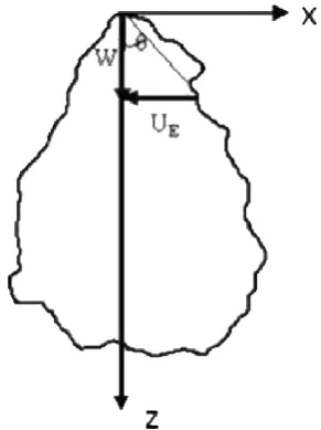
terms of the vertical velocityW:UE=αEW (Fig. 1).
There-fore, it is possible to calculate the entrainment coefficient as αE=UE/W. Closure of the equations is then possible
through the use of the entrainment constantαE.
Laboratory experiments have been performed to determine a range forαE. Morton et al. (1956) did some experiments
and they found a constant value ofαE=0.13, and proposed
this value as a universal constant. In the absence of a theory forαE, it has become common in geophysical problems to
use an arbitrary value of 0.09 without a clear physical basis. However, decades of experiments on plumes and jets do not support the assumption of a universal constant value forαE.
In fact, most authors use different entrainment coefficients for different discharge and/or environmental conditions. For example, in Tate (2002), Wright (1984) uses an entrainment coefficient of 0.30 for discharges of a jet issuing from an ax-isymmetric source under conditions of stratified and stagnant ambient waters, and a value of 0.14 for discharges of a plume under the same conditions. The estimates ofαE. The
entrain-ment coefficient αE also varies between 0.05 and 0.12
ac-cording to the direction of the buoyancy force, negatively or positively buoyant (Kaminski et al., 2005). In case of nega-tively buoyant jets the variation inαE=0.075±0.05 is rather
large as for plumes. In lazy plumes,αEis found to be around
0.12 (Hunt and Kaye, 2001). There appears to be consider-able variability in the values of the entrainment coefficient as Tate (2002) presents in his work. For more details about values for the entrainment coefficient see tables 3.4–3.7 of its work. Tate (2002) summarizes values for the entrainment coefficient for different model types that can be found in the literature and classified depending on the experimental con-ditions (axisymmetric or line source, jet or plume, stratified or unstratified ambient fluid, and flowing or stagnant ambi-ent fluid). For axisymmetric jets in an unstratified and
stag-Fig. 1. Schematic view of a forced downwards plume without
en-vironmental turbulence. The mean centerline speed is the vertical velocityWand radiusb. The plume entrains ambient fluid charac-terized by a mean entrainment velocityUE. The figure shows the
angle of the plumeθ.
nant ambient fluid, the mean entrainment is 0.080±0.029, and for axisymmetric plumes under the same conditions the mean entrainment is 0.110±0.034.
Therefore, the main limitation of Morton’s model is its as-sumption of a constant value forαE. As a consequence this
model cannot explain that the values ofαE for a jet and a
plume differ significantly, varying between 0.05 and 0.16, re-spectively (Kaminski et al., 2005), so a forced plume cannot be characterized by a single value, a constant entrainment co-efficient can only give approximate predictions (at first it will exhibit jet-like characteristics and ultimately it must exhibit plume-like characteristics).
Frick (1984) recognized that a more complex entrainment function is necessary in order to reproduce the results in lab-oratory and field experiments. Instead of usingW=UE/αE,
he establishes a difference between the shear entrainment,
(αE)shear, and the vortex entrainment, (αE)vortex. Until
re-cently, there was no theoretical explanation for the variation of αE. The model of Kaminski et al. (2005) explains these
variations and the role of both positive and negative buoy-ancy in the entrainment process is highlighted. The larger values ofαEin pure and lazy plumes are due to positive
buoy-ancy which enhances the entrainment of background fluid by promoting the formation of large-scale turbulence structure. Conversely, a negative buoyancy force inhibits entrainment and reducesαE (Kaminski et al., 2005). On the other hand,
the variations within pure jets and pure plumes can be ex-plained by the downstream evolution of each flow to a state of self-similarity (Carazzo et al., 2006).
of the flow where inertial forces dominate compared with the buoyancy-dominated region far from the source (Morton, 1959). To account for this evolution, some authors proposed empirical or semi-empirical parametrizations allowingαEto
vary according to the ratio of the buoyancy and inertia forces:
αE=αj− αj−αp
Fr
p
Fr
2
, (5)
where Fr is the Froude number and Frpis the constant Froude
number for a pure plume in a uniform environment, andαj
andαpare arbitrary constant values ofαEfor pure jets and
pure plumes, respectively (Lee and Chu, 2003). The values of the entrainment coefficient that best fit the data fall between the bounds formed by the values ofαEfor pure jets and pure
plumes in uniform environments (Carazzo et al., 2006) ex-cept at large distances from the source whereαEvalues are
even smaller than those predicted for a pure jet.
The variable entrainment models may easily be adapted to a good agreement with small-scale laboratory experiments, with the Morton et al. (1956) model obtaining reasonable predictions at both small and at large distances from the source. On the other hand, they are also useful with geo-physical or environmental turbulent plumes such as volcanic plumes on Earth or other planets, atmospheric sources of pol-lution, sewer discharge plants near the coast or submarine plumes rising from hydrothermal vents.
3 Experimental setup
The aim of the experimental procedure is to generate a tur-bulent axysimmetric plume, descending from a finite source in an unstratified and stagnant environment fluid and control-ling its position and its physical characteristics as buoyancy and momentum fluxes (see Table 1). The experiments con-sisted of releasing a denser fluid downwards from a small nozzle, with a diameter D of 0.6 cm and an area So of
0.2827 cm2, into a stationary body of water that was con-tained in a glass tank of dimensions 32 cm high by 25 cm by 25 cm. This water layer is designated as the lighter layer with a heighthL=17 cm and a densityρL=1.0 g cm−3. On
top of this lighter layer, a system made of two metacrylic boxes is placed (Fig. 2). The bottoms of the boxes are pierced with one regulated orifice that is at a height Ho from the
lighter layer and represents the position of the injection ori-fice. These boxes contain the denser layer that reaches a heighthD=1.134 cm and a densityρD(López, 2004; López
et al., 2008). The starting point of the plume is located at a heightHo, which takes the values 0, 2, 3, 6, and 8 cm. For
eachHo, we use four different potassium permanganate
solu-tions as the releasing fluids with an intense purple color and a volume of 500 cm3. This provides the following range of At-wood numbers: 0.001, 0.0025, 0.005, and 0.01. Denser fluid with momentum and buoyancy fluxes is discharged from the orifice continuously at a flow rate ofVo=8.40 cm3s−1. A
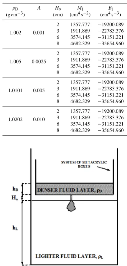
Table 1. The 16 different experimental conditions of the fluid
sys-tem. The density of the denser layer isρD.Ais the Atwood
num-ber. The location of the ejecting orifice isHo. The buoyancy and
momentum fluxes at the impinging surface areBlandMl.
ρD A Ho Ml Bl
(g cm−3) (cm) (cm4s−2) (cm4s−3)
1.002 0.001
2 1357.777 −19200.089 3 1911.869 −22783.376 6 3574.145 −31151.221 8 4682.329 −35654.960
1.005 0.0025
2 1357.777 −19200.089 3 1911.869 −22783.376 6 3574.145 −31151.221 8 4682.329 −35654.960
1.0101 0.005
2 1357.777 −19200.089 3 1911.869 −22783.376 6 3574.145 −31151.221 8 4682.329 −35654.960
1.0202 0.010
2 1357.777 −19200.089 3 1911.869 −22783.376 6 3574.145 −31151.221 8 4682.329 −35654.960
Fig. 2. Schematic diagram of the experimental configuration that
shows the initial state of the fluid system with a starting forced plume.hLandρLare the height and the density of the lighter layer
of fluid;hDandρDare the height and the density of the denser layer
and the heightHois the source position and varies from 0 to 8 cm.
sketch of the experimental setup is given in Fig. 2 (López, 2004; López et al., 2008).
of the experiments are sequenced into frames using frame-sequencer software (640 by 480 pixels capturing an area of 25 by 18 cm). The registered images average the concentra-tion over the volume of the plume.
Table 1 lists the characteristics of the 16 different ex-perimental conditions of the fluid system and the generated plume. The rate of supply of buoyancy is the buoyancy flux of the plume at sourceBo, whose value is−8232 cm4s−3.
The buoyancy flux is negative because the discharge fluid is heavier than the ambient fluid. The rate of supply of momen-tum by the source is the momenmomen-tum flux at sourceMowhose
value is 249.593 cm4s−2. The denser fluid is injected through the orifice with these fluxes and impinges on the lighter layer.
BlandMl are the initial effective buoyancy and momentum
fluxes at the free surface of the lighter layer as a consequence of the conversion from potential energy to initial kinetic en-ergy of the plume.
3.1 Plume growth in steady environments
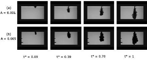
Plume occurs where fluid of different density from the ambi-ent fluid is injected, as the density of the effluambi-ent is heavier than its surrounding ambient fluid and, therefore, the buoy-ancy force is downward and the initial flow is directed ver-tically downwards in the same direction as the buoyancy forces. Figure 3 shows several sequences of digitized video images from two experiments under different source condi-tions wheret∗is the non-dimensional time defined ast∗= t
tc.
The timescaletc is the time that a plume spends in crossing
the distanceHo+hL(see Fig. 2):tc=
q
Ho+hL Ag .
Upon entering the ambient fluid flow, the denser fluid be-comes unstable and forms the axisymmetric plume at the center of the tank. As the plume is gravitationally unstable, it engulfs lighter fluid as it evolves, but the forced plume has different behaviors: jet-like characteristics depending on its initial mass and momentum fluxes, and plume-like charac-teristics depending on its initial buoyancy flux. If we use the Fischer characteristic lengthLm(Fischer et al., 1979) and its
related dimensionless parameterz/Lm, it is possible to
an-alyze the degree of jet-like and plume-like behaviors of the forced plume. Our Fischer’s length ranges from 10.94 for the smallest Atwood number (A=0.001) to 3.46 for the greatest Atwood number (A=0.01).
A forced plume can be considered as a pure jet atLz
m <0.5
and as a pure plume atLz
m >5; when 0.5< z
Lm <5 we have
the transition of the forced plume (Fischer et al., 1979). For our plume experiments, z/Lm ranges from 0.165 (for the
smallestz, Atwood numberAand initial Richardson num-ber Rio) to 1.879 (for the greatestz,A, and Rio). Then, the
dynamical behavior of the fluid flow modifies from a pure jet-like to a forced plume in a transition state. Moreover, for a given experiment or fixed buoyancy and source position, the non-dimensional quantityz/Lmincreases with time.
Fig. 3. Time evolution of one turbulent plume through its frame
sequences corresponding to two experiments with different At-wood numbersAmade with the same height for the starting point
Ho=3 cm. (a)A=0.001 and (b)A=0.005 for non-dimensional
timet∗=0.09, 0.39, 0.70, and 1.
Buoyancy is said to be dominant after some distance, which verifiesz >5Lm, which is different for each
experi-ment. Usually, after ten to twenty source diameters the buoy-ancy dominates the flow. At this stage the entrainment of the ambient fluid directed through the border of the turbulent plume is more effective. The sides of the plume are zones with strong shears, which generate Kelvin–Helmholtz in-stabilities, and secondary Rayleigh–Taylor instabilities may also appear at the front of the convective plume.
Finally, the plume advance spreads sideways as it evolves until it reaches the physical contours of the tank which limit the development of the plume generating a gravity current and an overturn of the fluid system.
4 Quantitative results: velocity fields and entrainment coefficient variations
We use the PIV (particle image velocimetry) method to un-derstand the behavior of turbulent plume based on our ve-locity field measurements. We calculate veve-locity PDFs with the DigiFlow program (Matulka et al., 2008) using sequences from experiments that were videotaped. We analyze the evo-lution of the velocity fields visualizing different graphics, which can give us an idea about vertical velocity, the en-trainment velocity and the enen-trainment coefficient. The study of the velocity fields gives us information about the time progress of the turbulent plume, in which direction is the propagation of the plume or with what velocity is flowing. We can find its vertical velocity by looking at the length of the plume or entrainment velocity by looking at the width of the plume.
We calculate the vertical velocity as W=z/t [cm s−1],
where z is the length of the turbulent plume and t is the time of the propagation of the plume. The magnitudezi
mea-sures the length of the plume in each timeti. On the
Fig. 4. Time sequence of a turbulent plume experiment with Atwood
numberA=0.001 andHo=2 cm. The values ofz1,z2, andz3are
shown. (a) Plume att1∗=0.2, (b) plume att2∗=0.5, and (c) plume att3∗=1.0.
Fig. 5. Time sequence of a turbulent plume experiment with Atwood
numberA= 0.001 andHo=2 cm. The values ofx1,x2, andx3are
shown. (a) Plume att1∗=0.2, (b) plume att2∗=0.5, and (c) plume att3∗=1.0.
We calculate entrainment velocity asUE=x/t [cm s−1]
where thex is the width of the plume at the maximum point of it, and t time is the same as for the vertical velocity. Figure 5 shows the elements for the entrainment velocity cal-culation for the same selected plume as in Fig. 4. Therefore, it is possible to calculate the entrainment coefficient as de-fined in Sect. 2.1.
As a consequence of this procedure, it is possible to an-alyze the time evolution of the vertical velocityW, the en-trainment velocity UE and the entrainment coefficient αE.
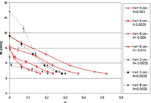
Figure 6 shows the time evolution of the vertical velocityW
under different source conditions (varying Atwood numbers with a fixedHoand source positionsHowith a fixed Atwood
number).
The time variation of vertical velocity has a greater dis-persion at early times (Fig. 6) and W ranges from 12 to 27 cm s−1. Close to the end of the experiment, the vertical velocity has no dispersion and tends to a constant value close to 6.5 cm s−1 independently of Atwood numberAandHo.
This limit vertical velocity does not depend on source condi-tions. Therefore, differences are only evident at early times and there are no differences at the end of the experiments for all source conditions.
Fig. 6. Time evolution of the vertical velocityW under different source conditions.
Fig. 7. Time evolution of the entrainment velocityUEunder
differ-ent source conditions.
The entrainment velocity also has dispersion at initial times (Fig. 7), but the time behavior is slightly different if we compare it with the evolution of the vertical velocity, es-pecially at the end of the experiment. The dispersion at early times ranges from 6 to 10.5 cm s−1and it ranges from 2.5 to 3.3 cm s−1at the end of the experiment. We observe that the data dispersion decreases in time. We observe that the en-trainment velocity decreases in time in a similar way for all the source conditions (Fig. 7). The most evident difference is that there is no limit value forUEclose to the end of the
experiment: different values of the source conditions (Aand
Ho) have differentUE.
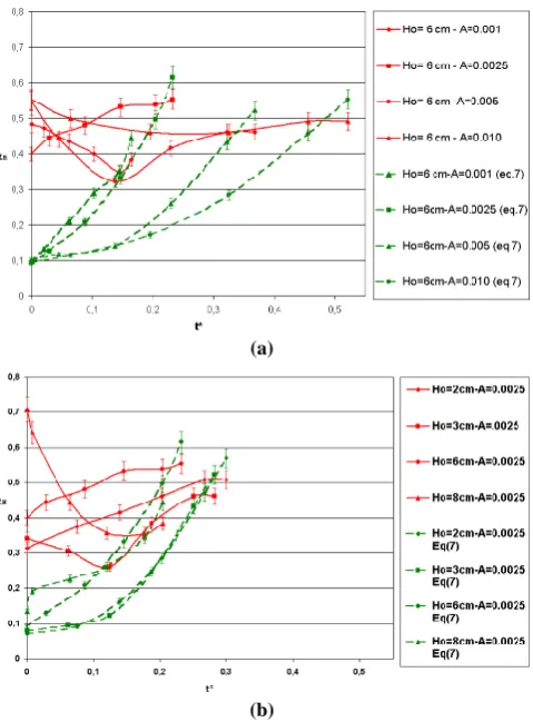
The entrainment coefficient also has a marked dispersion at initial times (Fig. 8) and is less important close to the end of the experiment. At early times, the entrainment coeffi-cient has an important dispersion and ranges between 0.40 and 0.55 for variable Atwood number experiments and be-tween 0.31 and 0.71 for variableHo experiments. Close to
(a)
(b)
Fig. 8. Time evolution of the entrainment coefficientαEunder
dif-ferent experimental conditions. (a) With a fixedHo=6 cm; dashed
lines represent the evaluation of Eq. (7) for the same source con-ditions. (b) With a fixed Atwood numberA=0.0025; dashed lines represent the evaluation of Eq. (7) for the same source conditions.
(0.39, 0.55) for the second ones. Therefore, the entrainment coefficientαEdoes not tend to a constant value and shows a
time evolution within the same plume and for all the source conditions.
A verification that the time evolution of the entrainment coefficient exits within the same plume is to measure the angle of the plume because of the following relationαE≈
tan(θ ) (Fig. 1). Figure 9 shows the time evolution of the plume angle for an experiment withHo=2.5 cm andA=
0.03. From these data of a measured angle, θ, the follow-ing empirical linear fit is deduced:θ=8.34+10.27t∗. The value of the coefficient of determinationR2is 0.75, which indicates that the presented linear model explains 75 % of the variability in our angle data set. From the same data of the plume angle it is possible to deduce a better non-linear fit that is a log fitθ=16.86+3.40 log(t∗). Figure 9 shows this log fit (dashed line). This non-linear log model explains 91 % of the variability in our angle data set. Therefore, the angle of the plume angle that is indirectly related to the entrainment coefficient is not constant in time.
Fig. 9. Time evolution of the angleθ(◦) of the plume for an experi-ment with a fixedHo=2.5 cm and Atwood numberA=0.03. The
log fit (dashed line) is also shown.
5 Brief discussion and future work
The original model of Morton et al. (1956) is not sufficient to explain all the experimental and geophysical data about plumes, as was clearly stated in Sect. 2.1. The present labo-ratory experimental work was motivated by the idea of veri-fying if the entrainment coefficient varies in time within the same plume and changes with source conditions. Our results about the behavior of the entrainment coefficient verify all these assumptions.
We have considered the topological and geometrical ef-fects affecting the initial evolution of jets/plumes that also appear in nature. The role of ambient turbulence and of en-vironmental buoyancy as discussed by Redondo et al. (1995) and Redondo and Yagüe (1994) will be considered in future work. Here we present an experimental study where we mea-sure the entrainment coefficient, analyzing its time behavior within the same plume and under different source conditions (Fig. 8). We also study the behavior of vertical and axisym-metric velocity at early times under different source condi-tions (Figs. 6 and 7).
In general, vertical velocities are greater for variableHo
experiments (Fig. 6), i.e., the source positionHohas an effect
on vertical velocity. Close to the end of the experiment, there is a limit to the vertical velocity for the plume (6.5 cm s−1) that is not affected by the buoyancyAand the location of the ejection orificeHo, i.e., it is independent of the source
con-ditions. The model of Morton et al. (1956) gives the mean vertical speed of a plume W∝ 1
b1/3 whereb is the radius
The behavior of the entrainment velocity is represented by Fig. 7. The entrainment velocity decreases in time in a simi-lar way for all source conditions. Given the definition of the entrainment coefficient and the relation for the mean verti-cal speed of the model of Morton et al. (1956), it is possi-ble to suppose that the entrainment velocity decreases in a similar way (UE∝b11/3) if the entrainment coefficient is
sup-posed constant. For these experiments, there is no clear lim-iting value for UE close to the end of the experiment. For
variable Atwood number experiments, the entrainment ve-locityUE increases with the Atwood number. As the
posi-tion of the orifice Ho is fixed, only the buoyancy changes
by means of the Atwood numberA; therefore, the increase in buoyancy increases the entrainment velocity. For variable
Hoexperiments, the entrainment velocityUEalso decreases
in time (Fig. 7). As buoyancy is fixed, only the source loca-tion changes, but the entrainment velocity does not clearly increase with the variation in the source location.
Finally, we conclude that the entrainment velocity in-creases with the Atwood number,A, and it is not so sensitive to the source location,Ho.
In this turbulent plume study we have observed that the en-trainment coefficient has important variations in time within the same plume and also with the initial buoyancy and source position conditions, as Fig. 8 shows. At early times, the en-trainment coefficient has an important dispersion and close to the end of the experiment, the dispersion of the entrainment coefficient is less important, as in all cases the behavior is plume-like. Although the dispersion has decreased in time, it is clear that the entrainment coefficientαE does not tend
to a constant value and has a time evolution within the same plume and for all the source conditions. This is our main re-sult, which differs from other authors who compare different plumes or jets, or plumes and jets.
This result has an important theoretical implication be-cause in generating the asymptotic equations for a buoyant fluid discharged into an ambient fluid (may be flowing or stagnant, stratified or unstratified), the entrainment coeffi-cientαEis assumed to be independent of time (Tate, 2002).
Therefore, if a time variation forαEis confirmed, the
mathe-matical treatment to deduce the asymptotic equations should change to introduce a time dependence in the entrainment coefficient function. More experimental work is necessary to look for this time dependence and to achieve this aim, and in particular to understand the important differences between axisymmetric plumes within a 3-D space and line plumes that exhibit a 2-D geometry.
Figure 8b shows the time behavior of the entrainment co-efficient for variableHoexperiments. As Atwood numberA
is constant, the effect of buoyancy is constant and only the effect of the source location is considered. The behavior of the entrainment coefficient is non-regular in time and varies with the source position,Ho. As the location of the source is
higher, the coefficientαEis greater at early time and also at
the end of the experiment.
Moreover, the measured entrainment coefficient has con-siderable variability, more evident at initial steps of the experiments. We also observe that the entrainment coeffi-cient values are greater than the typical value of Morton et al. (1956) and the values for plumes (between 0.085 and 0.16) and jets (between 0.051 and 0.07). Considering all the results, we have evaluated Eq. (5) using our data. To evaluate the equation we write the Froude number Fr in terms of the Atwood numberA. The Froude number Fr is a dimensionless quantity that measures the relative importance of the inertial and gravitational effects on a fluid flow. The local densimet-ric Froude number of a plume based on the centerline values of the vertical velocity and reduced gravity is:
Fr= W
q Mρ
¯ ρ g b
=√ W
2A g b, (6)
whereMρis the density difference between plume and ambi-ent fluids (ρD−ρL) andρ¯is the average fluid density.
There-fore, Eq. (5) would be:
αE=αj− αj−αp
2Fr2pA g b W
!2
, (7)
where Frp=4.5,αj=0.057 (for a round jet) andαp=0.09
(for a round plume) (Lee and Chu, 2003). Equation (7) shows that the entrainment coefficientαE depends on the Atwood
numberA, the plume vertical velocityW and the plume ra-diusb.
Figure 8 shows the results of the evaluation of Eq. (7) for variable Atwood numberA(Fig. 8a, dashed lines) and vari-able source positionHo(Fig. 8b, dashed lines) experiments.
For both kind of experiments, a similar behavior appears: the evaluated entrainment coefficient always increases in time. Therefore, Eq. (7) also predicts a time change forαE.
An-other conclusion is that our experimental entrainment coeffi-cient is clearly greater (and has more dispersion) than that evaluated by Eq. (7) at early times. Our greater values of
αE could be related to the plume characteristics. The plume
is not laminar and it presents turbulence from the starting point (with momentum and buoyancy fluxes). Another rea-son could be that the values of the parametersαj andαp in
Eq. (7) are not the most adequate for our configuration. Our measurements are still greater close to the end of the experi-ments, but the difference in values is less important. Really, at the end of the experiment, all the values (the experimental ones and those evaluated from Eq. 7) range between 0.38 and 0.62.
(López et al., 2008). As dimensions of volume, momen-tum and buoyancy fluxes for 2-D are[Q] =L2T−1,[M] =
L3T−2,[B] =L3T−3and for 3-D they are[Q] =L3T−1, [M] =L4T−2,[B] =L4T−3, then the respective jet-plume transition length scales are (Redondo and Yagüe, 1994): ŁJ P2D=C2DM B2/3, ŁJ P3D=C3DM3/4B−1/2. (8)
So their mixing front time evolutions arez∝B1/3tfor 2-D andz∝B1/4t3/4for 3-D. This is verified in Landel et al. (2012) as well as in Carazzo et al. (2006) and also indicates that Rayleigh–Taylor or top-heavy initial mixing can be very efficient.
In the case of turbulent or stratified environments, local entrainment values are strongly dependent on height and it is still necessary to evaluate higher order effects such as lo-cal variability, non-homogeneity and intermittency. It is in-teresting to use dimensional analysis to derive a general non-dimensional parameter space for use in the environment be-cause observations seldom correspond to equilibrium.
For 2-D or line sources we use wU, N MU3 whereN is the buoyancy frequency, and for 3-D axisymmetric sources we have wU, U4M
B2 or U4
N B as a density Froude number that ex-presses the relative importance of kinetic to potential ener-gies. In both cases (2- and 3-D)N M/Bis a measure of the relative importance of momentum and buoyant fluxes in the presence of stratification. Finally,U4/(N2M)represents the relative importance of the motion at buoyant fluid compared with an initial jet.
The non-dimensional parameter space is useful for gen-erating a 4-D surface that represents the variation of the entrainment coefficient, because there is no constant value forαE (for a single experiment under the same conditions,
the entrainment coefficient changes due to intermittency, changes from jet to plume or from a 2- to a 3-D situation). Further work should analyze intermittency and extend the entrainment assumptions to include higher order moments of the velocity and density moments and structure functions (Vindel at al., 2008) following an experimental procedure de-scribed in Mahjoub et al. (1998).
6 Conclusions
In this experimental study of a turbulent plume, our main re-sult is that the entrainment coefficient is not a constant and clearly varies in time within the same plume independently of the buoyancy and the source position. Other authors com-pare different plumes or different jets, or plume and jet ex-periments, but our result is for a given plume experiment. We also observe that the time evolution of the entrainment coefficient appears with different initial experimental forcing conditions.
Moreover, the measured entrainment coefficient has con-siderable variability, more evident at initial steps of the ex-periments. We find as in Carazzo et al. (2006) that, at early
times, the entrainment coefficient has an important disper-sion and ranges between 0.26 and 0.9 for variable Atwood number experiments and between 0.16 and 0.55 for variable source position experiments. It is interesting to use these al-ternative descriptors instead of the usual momentum fluxes of volume, momentum and buoyancy because of an eas-ier comparison with the highest initial mixing ability of the Rayleigh–Taylor instability (López et al., 2008). It is also ob-served that close to the end of the experiment, the dispersion of the entrainment coefficient is less important; it ranges be-tween (0.17, 0.46) for variable Atwood number experiments and (0.37, 0.49) for variable source location experiments. The values of the coefficient are greater than the typical value of Morton et al. (1956) (0.13) and usually measured or cal-culated entrainment coefficients (but it is not an exception because List (1982) presents values of 0.57 and (0.47, 0.88), or Frick (1984) a value of 0.56).
It is equivalent to consider an initial condition parameter of (Qo,Mo,Bo) or (Ho,Vo,Ao) to determine the initial effects
including the angle of spread of the jet/plume, but the variabi-lity of ambient conditions seems also to need a complex and extended parameter space as discussed above. In terms of a generalized turbulent Schmidt or Prandtl number with values between 0.5 and 2, the jets (highHoandA) reach their
equi-librium conditions faster than the plumes, in agreement with Carazzo et al. (2006) for 3-D flows. In clear 2-D situations the sideways meandering of the jets/plumes increases the ef-fective entrainment and the angles as indicated by Landel et al. (2012). Therefore it is necessary to provide more com-plex models of entrainment that depend on the jet to plume lengths for 2- and 3-D as well as other factors.
Acknowledgements. The authors would like to thank the ICMAT
Severo Ochoa project SEV-2011-0087 for its financial support. The authors would also like to thank the help of M. García Velarde and the facilities offered by the Pluri-Disciplinary Institute of the Complutense University of Madrid. We also acknowledge the help of the European Community under project Multi-scale complex fluid flows and interfacial phenomena (PITN-GA-2008-214919). Thanks are also due to ERCOFTAC (PELNoT, SIG 14). We acknowledge the referees for assisting in evaluating this paper.
Edited by: A. M. Mancho
Reviewed by: P. Fraunie, M. Jellinek, and two anonymous referees
References
Carazzo, G., Kaminski, E., and Tait, S.: The route to self-similarity in turbulent jets and plumes, J. Fluid. Mech., 547, 137–148, 2006.
Fischer, H. B., List, E. J., Koh, R. C., Imberger, J., and Brooks, N. H.: Mixing in inland and coastal waters, Academic Press Inc. (London) Ltd., 1979.
Frick, W. E.: Non-empirical closure of the plume equations, Atmos. Environ., 18, 653–662, 1984.
Houghton, H. G. and Cramer, H. E.: A theory of entrainment in convective currents, J. Meteorol., 8, 95–102, 1951.
Hunt, G. R. and Kaye, N. G.: Virtual origin correction for lazy tur-bulent plumes, J. Fluid. Mech., 435, 377–396, 2001.
Kaminski, E., Tait, S., And Carazzo, G.: Turbulent entraiment in jets with arbitrary buoyancy, J. Fluid. Mech., 526, 361–376, 2005. Landel, J. R., Caulfield, C. P., and Woods, A.: Meandering due to
large eddies and the statistically self-similar dynamics of quasi-two-dimensional jets, J. Fluid Mech., 692, 347–368, 2012. Lee, J. H. W. and Chu, V. H.: Turbulent jets and plumes: A
la-grangian approach, Kluwer Academic Publishers, the Nether-lands, 2003.
List, E. J.: Turbulent jets and plumes, Annu. Rev. Fluid Mech. 14, 189–212, 1982.
López, P.: Turbulent mixing by gravitational convection: exper-imental modelling and application to atmospheric situations, Ph.D. thesis, Complutense University of Madrid, Spain, 2004. López, P., Cano, J. L., and Redondo, J. M.: An experimental model
of mixing processes generated by an array of top-heavy turbulent plumes, Il Nuovo Cimento, 31 C, 679–698, 2008.
Mahjoub, O. B., Redondo, J. M., and Babiano, A.: Structure func-tions in complex flows, Appl. Sci. Res., 59, 299–313, 1998. Matulka, A., Redondo, J. M., and Carrillo, A.: Experiments in
strat-ified and rotating decaying 2D flows, Il Nuovo Cimento, 31 C, 757–770, 2008.
Morton, B. R.: Forced plumes, J. Fluid Mech., 5, 151–163, 1959. Morton, B. R.: The choice of conservation equations for plume
models, J. Geophys. Res., 30, 7409–7416, 1971.
Morton, B. R., Taylor, G. I., and Turner, J. S.: Turbulent gravita-tional convection from maintained and instantaneous sources, P. Roy. Soc. Lond. A Mat., 234, 1–23, 1956.
Nielsen, P. V.: Displacement ventilation-theory and design, Ph.D. thesis, Aalborg University, Aalborg, Denmark, 1993.
Redondo, J. M., Fernando, J. H., And Pares, S.: Cloud entrain-ment by internal or external turbulence, in: Mixing in Geophys-ical Flows, edited by: Redondo, J. M. and Metais, O., CIMNE, Barcelona, 1995.
Redondo, J. M. and Yagüe, C.: Plume entrainment in stratified flows, in: Recent advances in the fluid mechanics of turbulent jets and plumes, edited by: Davies, P. A. and Valente-Neves, M. J., NATO ASI Series E: Applied Sciences, 255, 209–222, 1994. Squires, P. and Turner, J. S.: An entraining jet model for
cumulo-nimbus updraughts, Tellus, XIV, 422–434, 1962.
Sreenivas, K. R. and Prasap, A. K.: Vortex dynamics model for entrainment in jets and plumes, Phys. Fluids, 12, 2101, doi:10.1063/1.870455, 2000.
Stommel, H.: Entrainment of air into a cumulus cloud, J. Meteorol., 4, 91–94, 1947.
Tate, P. M.: The rise and dilution of buoyant jets and their behaviour in an internal wave field, Ph.D. thesis, University of New South Wales, Sydney, Australia, 2002.
Turner, J. S.: The starting plume in neutral surroundings, J. Fluid. Mech., 13, 356–368, 1962.
Turner, J. S.: Turbulent entrainment: the development of the en-trainment assumption and its application to geophysical flows, J. Fluid Mech., 173, 431–471, 1986.
Vindel, J. M., Yagüe, C., and Redondo, J. M.: Relationship be-tween intermittency and stratfication, Il Nuovo Cimento, 31 C, 669–678, 2008.