David F. Hill1, Elizabeth A. Burakowski2, Ryan L. Crumley3, Julia Keon1, J. Michelle Hu4, Anthony A. Arendt5, Katreen Wikstrom Jones6, and Gabriel J. Wolken6,7
1Civil and Construction Engineering, Oregon State University, Corvallis, OR, USA
2Institute for the Study of Earth, Oceans, and Space, University of New Hampshire, Durham, NH, USA 3Water Resources Graduate Program, Oregon State University, Corvallis, OR, USA
4Civil and Environmental Engineering, University of Washington, Seattle, WA, USA 5Applied Physics Laboratory, University of Washington, Seattle, WA, USA
6Alaska Division of Geological & Geophysical Surveys, Fairbanks, AK, USA
7International Arctic Research Center, University of Alaska Fairbanks, Fairbanks, AK, USA Correspondence:David F. Hill (david.hill@oregonstate.edu)
Received: 21 December 2018 – Discussion started: 23 January 2019 Revised: 3 June 2019 – Accepted: 10 June 2019 – Published: 4 July 2019
Abstract. We present a simple method that allows snow depth measurements to be converted to snow water equiv-alent (SWE) estimates. These estimates are useful to indi-viduals interested in water resources, ecological function, and avalanche forecasting. They can also be assimilated into models to help improve predictions of total water volumes over large regions. The conversion of depth to SWE is partic-ularly valuable since snow depth measurements are far more numerous than costlier and more complex SWE measure-ments. Our model regresses SWE against snow depth (h), day of water year (DOY) and climatological (30-year nor-mal) values for winter (December, January, February) pre-cipitation (PPTWT), and the difference (TD) between mean temperature of the warmest month and mean temperature of the coldest month, producing a power-law relationship. Re-lying on climatological normals rather than weather data for a given year allows our model to be applied at measurement sites lacking a weather station. Separate equations are ob-tained for the accumulation and the ablation phases of the snowpack. The model is validated against a large database of snow pillow measurements and yields a bias in SWE of less than 2 mm and a root-mean-squared error (RMSE) in SWE of less than 60 mm. The model is additionally validated against two completely independent sets of data: one from western North America and one from the northeastern United States. Finally, the results are compared with three other models for
bulk density that have varying degrees of complexity and that were built in multiple geographic regions. The results show that the model described in this paper has the best perfor-mance for the validation data sets.
1 Introduction
In many parts of the world, snow plays a leading-order role in the hydrological cycle (USACE, 1956; Mote et al., 2018). Accurate information about the spatial and temporal distri-bution of snow water equivalent (SWE) is useful to many stakeholders (water resource planners, avalanche forecasters, aquatic ecologists, etc.), but can be time consuming and ex-pensive to obtain.
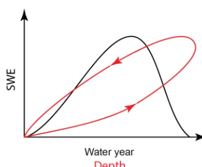
Figure 1.Conceptual sketch of the evolution of snow water equiva-lent (SWE) over the course of a water year (black line). Also shown is the evolution of SWE with snowpack depth over a water year (red line). Note the hysteresis loop due to the densification of the snowpack.
sites are not representative of the lowest or highest eleva-tion bands within mountainous regions (Molotch and Bales, 2006). In the western United States (USA), the Natural Re-sources Conservation Service (NRCS) operates a large net-work of snow telemetry (SNOTEL) sites, featuring snow pillows. The NRCS also operates the smaller Soil Climate Analysis Network (SCAN), which provides the only, and very limited, snow pillow SWE measurements in the eastern United States.
SWE can also be measured manually, using a snow cor-ing device that measures the weight of a known volume of snow to determine snow density (Church, 1933). These mea-surements are often one-off meamea-surements, or in the case of “snow courses” they are repeated weekly or monthly as a transect of measurements at a given location. The simplic-ity and portabilsimplic-ity of coring devices expand the range over which measurements can be collected, but it can be chal-lenging to apply these methods to deep snowpacks due to the limited length of standard coring devices. Note that there are numerous different styles of coring devices, including the Adirondack sampler and the Mt. Rose or Federal sam-pler (Church and Marr, 1937). The NRCS operates a large network of snow course sites (USDA, 2011) in the western United States.
There are a number of issues that affect the accuracy of both snow pillow and snow coring measurements. With cor-ing measurements, if the corcor-ing device is not carefully ex-tracted, a portion of the core may fall out of the device. Or, snow may become compressed in the coring device during insertion. These effects have led to varying conclusions, with some studies (e.g., Sturm et al., 2010) showing a low SWE bias and other studies (e.g., Goodison, 1978) showing a high SWE bias. As noted by Johnson et al. (2015) a good rule of thumb is that coring devices are accurate to around ±10 %.
Also, studies comparing different styles of snow samplers re-port statistically different results, suggesting that SWE mea-surements are sensitive to the design of the specific coring device, such as the presence of holes or slots, the device material, etc. (Beaumont and Work, 1963; Dixon and Boon, 2012). With snow pillows, some studies (e.g., Goodison et al., 1981) note that ice bridging can lead to low biases in measured SWE, with the snow surrounding the pillow partly supporting the snow over the pillow. Other studies (Johnson and Marks, 2004; Dressler et al., 2006; Johnson et al., 2015) note a more complex situation with SWE underreported at times, but overreported at other times. Note that when snow pillow data are evaluated, they are most commonly compared to coring measurements at the same location.
All methods of measuring SWE are challenged by the fact that SWE is a depth-integrated property of a snowpack. This is why the snowpack must be weighed, in the case of a snow pillow, or a core must be extracted from the surface to the ground. This measurement complexity makes it difficult to obtain SWE information with the spatial and temporal res-olution desired for watershed-scale studies. Other snowpack properties, such as the depthh, are much easier to measure. For example, using a graduated device such as a meterstick or an avalanche probe to measure the depth takes only sec-onds. Automating depth measurements at a fixed location can easily be done using low-cost ultrasonic devices (Goodison et al., 1984; Ryan et al., 2008). High-spatial-resolution mea-surements of snowpack depth are commonly made with lidar. One example of this is the Airborne Snow Observatory pro-gram (ASO; Painter et al., 2016). The comparatively high ex-pense of airborne lidar surveys typically limits measurements geographically (to a few basins) and temporally (weekly to monthly interval).
Given the relative ease in obtaining depth measurements, it is common to usehas a proxy for SWE. Figure 1 shows a conceptual sketch of the variation in SWE withhover a typical water year. Noting the arrows on the curve, we see that SWE is multivalued for eachh. This is due to the fact that the snowpack increases in density throughout the water year, producing a hysteresis loop in the curve. A large body of literature exists on the topic of how to converthto SWE. It is beyond the scope of this paper to provide a full review of these “bulk density equations”, where the density is given by ρb=SWE/ h. Instead, we refer readers to the useful com-parative review by Avanzi et al. (2015). Here, we prefer to discuss a limited number of previous studies that illustrate the spectrum of methodologies and complexities that can be used to determineρbor SWE.
it further to provide coefficients that depend on time and el-evation as well. They use a simple linear equation forρbin terms of h and the slope and intercept of the equation are given as monthly values, with three elevation bins for each month (36 pairs of coefficients). There is an additional con-tribution to the intercept (or “offset”) which is region-specific (one of seven regions).
These classifications, whether based on region, elevation, or season, are valuable since they acknowledge that all snow is not equal. McKay and Findlay (1971) discuss the con-trols that climate and vegetation exert on snow density, and Sturm et al. (2010) address this directly by developing a snow density equation where the coefficients depend upon the “snow class” (five classes). Sturm et al. (1995) explain the decision tree, based on temperature, precipitation, and wind speed, that leads to the classification. The temperature met-ric is the “cooling degree month” calculated during winter months only. Similarly, only precipitation falling during win-ter months was used in the classification. Finally, given the challenges in obtaining high-quality, high-spatial-resolution wind information, vegetation classification was used as a proxy. Using climatological values (rather than values for a given year), Sturm et al. (1995) were able to develop a global map of snow classification.
There are many other formulations for snow density that increase in complexity and data requirements. Meloysund et al. (2007) express ρb in terms of sub-daily measure-ments of relative humidity, wind characteristics, air pressure, and rainfall, as well as h and estimates of solar exposure (“sun hours”). McCreight and Small (2014) use daily snow depth measurements to develop their regression equation. They demonstrate improved performance over both Sturm et al. (2010) and Jonas et al. (2009). However, a key dif-ference between the McCreight and Small (2014) model and the others listed above is that the former cannot be ap-plied to a single snow depth measurement. Instead, it re-quires a continuous time series of depth measurements at a fixed location. Further increases in complexity are found in energy-balance snowpack models (SnowModel, Liston and Elder, 2006; VIC, Liang et al., 1994; DHSVM, Wigmosta et al., 1994, others), many of which use multilayer models to capture the vertical structure of the snowpack. While the particular details vary, these models generally require
high-TEL station, and is not part of a modeling effort, then bulk density equations and depth measurements are an excellent choice.
The present paper seeks to generalize the ideas of Mizukami and Perica (2008), Jonas et al. (2009), and Sturm et al. (2010). Specifically, our goal is to regress physical and environmental variables directly into the equations. In this way, environmental variability is handled in a continu-ous fashion rather than in a discrete way (model coefficients based on classes). The main motivation for this comes from evidence (e.g., Fig. 3 of Alford, 1967) that density can vary significantly over short distances on a given day. Bulk den-sity equations that rely solely on time completely miss this variability and equations that have coarse (model coefficients varying over either vertical bins or horizontal grids) spatial resolution may not fully capture it either.
Our approach is most similar to Mizukami and Perica (2008), Jonas et al. (2009), and Sturm et al. (2010) in that a minimum of information is needed for the calculations; we intentionally avoid approaches like Meloysund et al. (2007) and McCreight and Small (2014). This is because our in-terests are in convertinghmeasurements to SWE estimates in areas lacking weather instrumentation. The following sec-tions introduce the numerous data sets that were used in this study, outline the regression model adopted, and assess the performance of the model.
2 Methods 2.1 Data
2.1.1 Snow depth and snow water equivalent
In this section, we list sources of 1970–present snow data utilized for this study (Table 1). With regards to snow coring devices, we refer to them using the terminology preferred in the references describing the data sets.
USA NRCS snow telemetry and soil climate analysis networks
sub-daily observations ofh, SWE, and a variety of weather vari-ables (Fig. 2a). The periods of record are variable, but the vast majority of stations have a period of record in excess of 30 years. For this study, data from all SNOTEL sites in CONUS and Alaska and northeastern US SCAN sites (Fig. 2b) were obtained with the exception of sites whose period of record data were unavailable online. Only stations with both SWE andhdata were retained.
Canada (British Columbia) snow survey data
Goodison et al. (1987) note that Canada has no national digi-tal archive of snow observations from the many independent agencies that collect snow data and that snow data are in-stead managed provincially. The quantity and availability of the data vary considerably among the provinces. The Water Management Branch of the British Columbia (BC) Ministry of the Environment manages a comparatively dense network of Automated Snow Weather Stations (ASWSs) that measure SWE,h, accumulated precipitation, and other weather vari-ables (Fig. 2a). For this study, data from all British Columbia ASWS sites were initially obtained. As with the NRCS sta-tions, only ASWS stations with both SWE andhdata were retained.
USA NRCS snow course/aerial marker data
The snow survey program (USDA, 2008) dates to the 1930s and includes a large number of snow course and aerial marker sites (Fig. 2c) in western North America. While the measure-ment frequency is variable, it is most commonly monthly. To generate a data set for this study, data were extracted using the National Water and Climate Center Report Generator 2.0. This allows filtering by time period, elevation band, and other elements. All sites with data between 1980 and 2018 were in-cluded (Fig. 2c).
Northeastern US data
In addition to the data from the SCAN sites, snow data for this project from the northeastern United States come from two networks and three research sites (Fig. 2b). The Maine Cooperative Snow Survey (MCSS, 2018) network includesh and SWE data collected by the Maine Geological Survey, the United States Geological Survey, and numerous private con-tributors and contractors. MCSS snow data are collected us-ing the standard Federal or Adirondack snow samplus-ing tubes typically on a weekly to biweekly (every other week) sched-ule throughout the winter and spring, 1951–present. The New York Snow Survey network data were obtained from the National Oceanic and Atmospheric Administration’s North-east Regional Climate Center at Cornell University (NYSS, 2018). Similar to the MCSS, NYSS data are collected us-ing standard Federal or Adirondack snow samplus-ing tubes on weekly to biweekly schedules, 1938–present.
The Sleepers River, Vermont Research Watershed in Danville, Vermont (Shanley and Chalmers, 1999), is a USGS site that includes 15 stations with long-term weekly records ofhand SWE collected using Adirondack snow tubes. Most of the periods of record are 1981–present, with a few sta-tions going back to the 1960s. The sites include topographi-cally flat openings in conifer stands, old fields with shrub and grass, a hayfield, a pasture, and openings in mixed softwood– hardwood forests. The Hubbard Brook Experiment Forest (Campbell et al., 2010) has collected weekly snow observa-tions at the Station 2 rain gauge site, 1959–present. Measure-ment protocol collects 10 samples 2 m apart along a 20 m transect in a hardwood forest opening about 1/4 ha in size. At each sample location along the transect,hand SWE are measured using a Mt. Rose snow tube and the 10 samples are averaged for each transect. Finally, the Thompson Farm Re-search site includes a mixed hardwood forest site and an open pasture site (Burakowski et al., 2013, 2015). Daily (from 2011 to 2018), at each site, a snow core is extracted with an aluminum tube and weighed (tube+snow) using a digital hanging scale. The net weight of the snow is combined with the depth and the tube diameter to determineρb, similar to a Federal or Adirondack sampler.
Chugach Mountains (Alaska) data
In the spring of 2018, we conducted 3 weeks of fieldwork in the Chugach Mountains in coastal Alaska, near the city of Valdez (Fig. 2d–e). We measuredh using an avalanche probe at 71 sites along elevational transects during March, April, and May. The elevational transects ranged between 250 and 1100 m (net change along transect) and were acces-sible by ski and snowshoe travel. At each site, we measured hin eight locations within the surrounding 10 m2, resulting in a total of 550+snow depth measurements. These 71 sites were scattered across eight regions in order to capture spatial gradients that exist in the Chugach Mountains as the wetter, more dense maritime snow near the coast gradually changes to drier, less dense snow on the interior side.
Data preprocessing
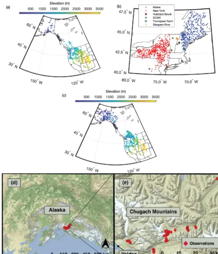
Figure 2.Distribution of measurement locations used in this study.(a)Western US and Canada snow pillow locations, with colors indicating station elevation in meters.(b)Northeastern United States snow pillow and snow course locations, with stations colored according to data source.(c)Western North America snow course and aerial marker locations, with colors indicating station elevation in meters.(d, e) Mea-surement sites in the Chugach Mountains, south-central Alaska.
strong correlation betweenhand SWE, we instead choose to use common outlier detection techniques for bivariate data.
The Mahalanobis distance (MD; De Maesschalck et al., 2000) quantifies how far a point lies from the mean of a bivariate distribution. The distances are in terms of the number of standard deviations along the respective
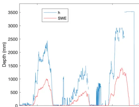
af-Figure 3.Sample time series of SWE andh from the Rex River (WA) SNOTEL station. Observations ofhat times when SWE is zero are likely spurious.
fected by outlier values. Therefore, it has been suggested (e.g., Leys et al., 2018) that a “robust” MD (RMD) be cal-culated. The RMD is essentially the MD calculated based on statistical properties of the distribution unaffected by the outliers. This can be done using the minimum covariance de-terminant (MCD) method as first introduced by Rousseeuw (1984).
Once RMDs have been calculated for a bivariate data set, there is the question of how large an RMD must be in or-der for the data point to be consior-dered an outlier. For bivari-ate normal data, the distribution of the square of the RMD isχ2(Gnanadesikan and Kettenring, 1972), withp(the di-mension of the data set) degrees of freedom. So, a rule for identifying outliers could be implemented by selecting as a threshold some arbitrary quantile (say 0.99) of χp2. For the current study, a threshold quantile of 0.999 was determined to be an appropriate compromise in terms of removing obvi-ous outlier points, yet retaining physically plausible results.
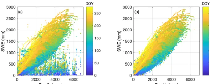
A scatter plot of SWE vs.hfor the SNOTEL data set from CONUS and AK reveals many nonphysical points, mostly when a very largehis reported for a very low SWE (Fig. 4a). Approximately 0.7 % of the original data points were re-moved in the preprocessing described above, creating a more physically plausible scatter plot (Fig. 4b). Note that the out-lier detection process was applied to each station individ-ually. The distribution of day of year (DOY) values of re-moved data points was broad, with a mean of 160 and a stan-dard deviation of 65. Note that the DOY origin is 1 Octo-ber. The same procedure was applied to the BC snow pillow, NRCS snow course, and northeastern US data sets as well (not shown). Table 1 summarizes useful information about the numerous data sets described above and indicates the fi-nal number of data points retained for each. We acknowledge that our process inevitably removes some valid data points,
but, as a small percentage of an already small 0.7 % removal rate, we judged this to be acceptable.
2.1.2 Climatological variables
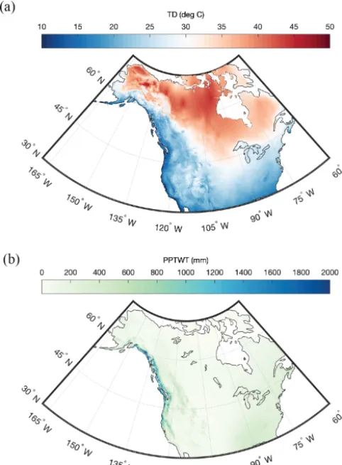
The 30-year climate normals at 1 km resolution for North America were obtained from the ClimateNA project (Wang et al., 2016). This project provides grids for minimum, max-imum, and mean temperature, and total precipitation for a given month. These grids are based on the PRISM normals (Daly et al., 1994) and are available for the periods 1961– 1990 and 1981–2010. For this study, the more recent cli-matology was used. The ClimateNA project also provides a wide array of derived bioclimatic variables, such as pre-cipitation as snow (PAS), frost-free period (FFP), mean an-nual relative humidity (RH), and others. Wang et al. (2012) summarize these additional variables and how they are de-rived. Figure 5 shows gridded maps of winter (sum of De-cember, January, February) precipitation (PPTWT) and the temperature difference (TD) between the mean temperature of the warmest month and the mean temperature of the cold-est month. The latter variable (TD) is a measure of continen-tality.
2.2 Regression model
In order to demonstrate the varying degrees of influence of explanatory variables, several regression models were con-structed. In each case, the model was built by randomly se-lecting 50 % of the paired SWE–h measurements from the aggregated CONUS, AK, and BC snow pillow data sets, ex-cluding the SCAN data. The model was then validated by applying it to the remaining 50 % of the data set and compar-ing the modeled SWE to the observed SWE for those points. We constructed a second version of the regression models by randomly selecting 50 % of the snow pillow stations and us-ing all of the data from those stations. The model was then validated by applying it to the data from the remaining 50 % of the stations. These two methods provided identical results, likely due to the very large sample size (N) of our data set. In all cases, thepvalues from the linear regression were 0, again due to the large sample size. Additional validation was performed with the northeastern US data sets (SCAN snow pillow and various snow coring data sets) and the NRCS snow course/aerial marker data set, which were completely left out of the model building process.
2.2.1 One-equation model
Figure 4.Scatter plot of SWE vs.hfor the complete SNOTEL data set before(a)and after(b)removing data points, following the method described in the section Chugach Mountains (Alaska) data. Symbols are colored by day of water year (DOY; 1 October is the origin).
Table 1.Summary of information about the data sets used in this study. Data sets in bold font were used to construct the regression model. The numbers of stations and data points reflect the post-processed data.
Data set name Data set type Number of Number and Precision percentage (h/SWE) retained of retained
stations data points
NRCS SNOTEL Snow pillow (SWE), ultrasonic(h) 791 1 900 000 (99.3 %) (12.7 mm/2.5 mm)
NRCS SCAN Snow pillow (SWE), ultrasonic (h) 5 7094 (97.8 %) (12.7 mm/2.5 mm)
British Columbia Snow Survey Snow pillow (SWE), ultrasonic(h) 31 61 000(97.5 %) (1 cm/1 mm)
NRCS Snow Survey Federal sampler/aerial marker 1085 116 000 (99.6 %) (12.7 mm/2.5 mm) for manual sampler (50.8 mm/n/a) for aerial marker
Maine Geological Survey Adirondack or Federal sampler (SWE andh) 431 28 000 (99.3 %) (12.7 mm/12.7 mm)
Hubbard Brook (Station 2), NH Mt. Rose sampler (SWE andh) 1 704 (99.4 %) (2.5 mm/2.5 mm)
Thompson Farm, NH Snow core (SWE andh) 2 988 (99.4 %) 12.7 mm/12.7 mm)
Sleepers River, VT Adirondack sampler 14 7214 (99.4 %) (12.7 mm/12.7 mm)
New York Snow Survey Adirondack or Federal sampler (SWE andh) 523 44 614 (98.2 %) (12.7 mm/12.7 mm)
Chugach Mountains, AK Avalanche probe (h) 71 71 (100 %) (1 cm)
express SWE as a power law, i.e.,
SWE=Aha1. (1)
This equation can be log-transformed into
log10(SWE)=log10(A)+a1log10(h) , (2) which immediately allows for simple linear regression methods to be applied. With both h and SWE expressed in millimeters, the obtained coefficients are (A, a1)= (0.146,1.102). Information on the performance of the model will be deferred until the results section.
2.2.2 Two-equation model
Recall from Figs. 1 and 4 that there is a hysteresis loop in the SWE–hrelationship. During the accumulation phase, snow
densities are relatively low. During the ablation phase, the densities are relatively high. So, the same snowpack depth is associated with two different SWEs, depending upon the time of year. The regression equation given above does not resolve this difference. This can be addressed by developing two separate regression equations, one for the accumulation (acc) phase and one for the ablation (abl) phase. This ap-proach takes the form of
SWEacc=Aha1; DOY<DOY∗, (3)
SWEabl=Bhb1; DOY≥DOY∗, (4)
Figure 5.Gridded maps of winter (December, January, February) precipitation (PPTWT) and temperature difference (TD) between the mean of the warmest month and the mean of the coldest month) for North America. Maps are for the 1981–2010 climatological pe-riod.
of peak SWE. Interannual variability results in a range of DOY∗values for a given site. Additionally, some sites, par-ticularly the SCAN sites in the northeastern United States, demonstrate multi-peak SWE profiles in some years. To re-duce model complexity, however, we investigated the use of a simple climatological (long-term average) value of DOY∗
at each site. For each snow pillow station, the average DOY∗
was computed over the period of record of that station. Anal-ysis of all of the stations revealed that this average DOY∗ was relatively well correlated with the climatological mean April maximum temperature (the average of the daily maxi-mums recorded in April;R2=0.7). However, subsequent re-gression analysis demonstrated that the SWE estimates were relatively insensitive to DOY∗and the best results were ac-tually obtained when DOY∗was uniformly set to 180 for all stations. Again, with both SWE andhin millimeters, the re-gression coefficients turn out to be(A, a1)=(0.150,1.082) and(B, b1)=(0.239,1.069)
As these two equations are discontinuous at DOY∗, they are blended smoothly together to produce the final two-equation model.
SWE=SWEacc 1
2 1−tanh
0.01
DOY−DOY∗
+SWEabl 1
2 1+tanh
0.01DOY−DOY∗ (5) The coefficient 0.01 in the tanh function controls the width of the blending window and was selected to minimize the root-mean-square error of the model estimates.
2.2.3 Two-equation model with climate parameters A final model was constructed by incorporating climatologi-cal variables. Again, the emphasis in this study is on methods that can be implemented at locations lacking the time series of weather variables that might be available at a weather or SNOTEL station. Climatological normals are unable to ac-count for interannual variability, but they do preserve the high spatial gradients in climate that can lead to spatial gradi-ents in snowpack characteristics. Stepwise linear regression was used to determine which variables to include in the re-gression. The initial list of potential variables included was SWE=f (h, z,PPTWT,PAS,TWT,TD,DOY,RH) , (6) where z is the elevation (m), PPTWT is the winter (sum of December, January, February) precipitation (mm), PAS is mean annual precipitation as snow (mm), TWT is the winter (December, January, February) mean temperature (◦C), TD is the difference between the mean temperature of the warmest month and the mean temperature of the coldest month (◦C),
DOY is the day of water year, and RH is the relative hu-midity (%). In the stepwise regression, explanatory variables were accepted only if they improved the adjustedR2value by 0.001. The result of the regression yielded
SWEacc=Aha1PPTWTa2TDa3DOYa4; DOY<DOY∗, (7)
SWEabl=Bhb1PPTWTb2TDb3DOYb4; DOY≥DOY∗, (8)
or, in log-transformed format, log10(SWEacc)
=log10(A)+a1log10(h)+a2log10(PPTWT) +a3log10(TD)+a4log10(DOY); DOY<DOY
∗
, (9) log10(SWEabl)
=log10(B)+b1log10(h)+b2log10(PPTWT)
a single equation for SWE spanning the entire water year. The obtained regression coefficients were(A, a1, a2, a3, a4) =(0.0533,0.9480,0.1701,−0.1314,0.2922)and(B, b1, b2, b3, b4) =(0.0481,1.0395,0.1699,−0.0461,0.1804). The physical interpretation of these coefficients is straightfor-ward. For example, botha2andb2are greater than zero. So, for two locations with equal h, DOY, and TD, the location with greater PPTWT will have a greater SWE and therefore density. These locations are typically maritime climates with wetter, denser snow. In contrast, botha3andb3are less than zero. Therefore, for two locations with equal h, DOY, and PPTWT, the location with greater TD (a more continental climate) will have a lower density, which is again an ex-pected result. These trends are similar in concept to Sturm et al. (2010), whose discrete snow classes (based on climate classes) indicate which snow will densify more rapidly.
3 Results
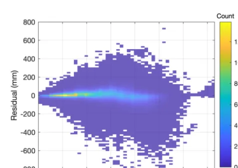
A comparison of the three regression models (one-equation model, Eq. 2; two-equation model, Eqs. 3–5; multivariable two-equation model, Eqs. 5, 7–8) is provided in Fig. 6. The left column shows scatter plots of modeled SWE to observed SWE for the validation data set with the 1:1 line shown in black. Figure 6a, c, and e show distributions of the model residuals. The vertical lines in Fig. 6b, d, and f show the mean error, or model bias. Visually, it is clear that the one-equation model performs relatively poorly with a large negative bias. This large negative bias is partially overcome by the two-equation model (Fig. 6c, d). The cloud of points is closer to the 1:1 line and the vertical black line indicating the mean error is closer to zero. In Fig. 6e, f, we see that the multivari-able two-equation model yields the best result by far. The residuals are now evenly distributed with a small bias. Sev-eral metrics of performance for the three models, including R2 (Pearson coefficient), bias, and root-mean-square error (RMSE), are provided in Table 2. Figure 7 shows the distri-bution of model residuals for the multivariable two-equation model as a function of DOY.
It is useful to also consider the model errors in a nondi-mensional way. Therefore, an RMSE was computed at each station location and normalized by the winter precipitation (PPTWT) at that location. Figure 8 shows the probability
Figure 6.Two-dimensional histograms (heat maps;a, c, e) of mod-eled vs. observed SWE and probability density functions(b, d, f)of the residuals for three simple models applied to the CONUS, AK, and BC snow pillow data. Warmer colors in the heat maps indicate greater density of points. The vertical lines in(b, d, f)indicate the location of the mean residual, or bias.(a, b)One-equation model (Sect. 2.2.1).(c, d)Two-equation model (Sect. 2.2.2).(e, f) Multi-variable two-equation model (Sect. 2.2.3).
Figure 8.Probability density function of snow pillow station root-mean-square error (RMSE) normalized by station winter precipita-tion (PPTWT) for the applicaprecipita-tion of the multivariable two-equaprecipita-tion model to the western North America snow pillow validation data set.
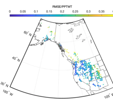
Figure 9. Spatial distribution of snow pillow station root-mean-square error (RMSE) normalized by station winter precipitation (PPTWT) for the application of the multivariable two-equation model to the western North America snow pillow validation data set.
density function of these normalized errors. The average RMSE is approximately 15 % of PPTWT with most values falling into the range of 5 %–30 %. The spatial distribution of these normalized errors is shown in Fig. 9. For the SNOTEL stations, it appears there is a slight regional trend, in terms of stations in continental climates (Rockies) having larger rela-tive errors than stations in maritime climates (Cascades). The British Columbia stations also show higher relative errors.
Table 3.Model parameters by snow class for Sturm et al. (2010).
Snow class ρmax ρ0 k1 k2
(g cm−3) (g cm−3) (cm−1) (cm−1)
Alpine 0.5975 0.2237 0.0012 0.0038 Maritime 0.5979 0.2578 0.0010 0.0038 Prairie 0.5941 0.2332 0.0016 0.0031 Tundra 0.3630 0.2425 0.0029 0.0049
Taiga 0.2170 0.2170 0.0000 0.0000
3.1 Results for snow classes
A key objective of this study is to regress climatological in-formation in a continuous rather than a discrete way. The work by Sturm et al. (2010) therefore provides a valuable point of comparison. In that study, the authors developed the following equation for densityρb:
ρb=(ρmax−ρ0)
h
1−e(−k1h−k2DOY)i+ρ
0, (11)
whereρ0is the initial density,ρmaxis the maximum or “final” density (end of water year),k1 andk2 are coefficients, and DOY in this case begins on 1 January. This means that their DOY for 1 October is−92. The coefficients vary with snow class and the values determined by Sturm et al. (2010) are shown in Table 3.
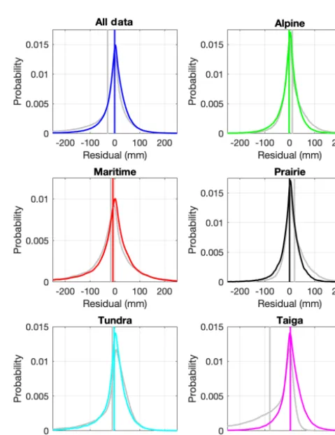
To make a comparison, the snow class for each SNOTEL and British Columbia snow survey (rows 1 and 3 of Table 1) site was determined using a 1 km snow class grid (Sturm et al., 2010). The aggregated data set from these stations was made up of 27 % alpine, 14 % maritime, 10 % prairie, 11 % tundra, and 38 % taiga data points. Equation (11) was then used to estimate snow density (and then SWE) for every point in the validation data set described in Sect. 2.2. Figure 10 compares the SWE estimates from the Sturm model and from the current multivariable, two-equation model (Eqs. 5, 7–8). The upper left panel of Fig. 10 shows all of the data, and the remaining panels show the results for each snow class. In all cases, the current model provides better estimates (narrower cloud of points; closer to the 1:1 line). Plots of the residuals by snow class are provided in Fig. 11, giving an indication of the bias of each model for each snow class. Summaries of the model performance, broken out by snow class, are given in Table 4. The current model has smaller biases and RMSEs for each snow class.
3.2 Comparison to Pistocchi (2016)
In order to provide an additional comparison, the simple model of Pistocchi (2016) was also applied to the validation data set. His model calculates the bulk density as
ρb=ρ0+K (DOY+61) , (12)
Novem-Figure 10.Comparison of the multivariable, two-equation model of the current study with the model of Sturm et al. (2010), applied to the western North America snow pillow validation data set. The subpanels show modeled SWE vs. observed SWE for all of the data binned together, as well as for the data broken out by the snow classes identified by Sturm et al. (1995). The gray symbols show the Sturm result and the transparent heat maps (warmer colors indi-cate greater density of points) show the current result.
ber. Application of this model to the validation data set yields a bias of 55 mm and an RMSE of 94 mm. These results are comparable to the Sturm et al. (2010) model, with a larger bias but smaller RMSE.
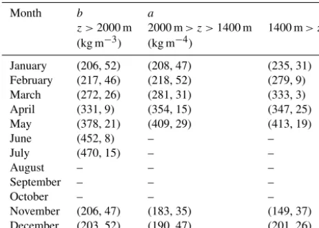
Table 5.Model coefficients(b, a)for the Jonas et al. (2009) model.
Month b a
z >2000 m 2000 m> z >1400 m 1400 m> z (kg m−3) (kg m−4)
January (206, 52) (208, 47) (235, 31) February (217, 46) (218, 52) (279, 9) March (272, 26) (281, 31) (333, 3) April (331, 9) (354, 15) (347, 25) May (378, 21) (409, 29) (413, 19) June (452, 8) – – July (470, 15) – –
August – – –
September – – –
October – – –
November (206, 47) (183, 35) (149, 37) December (203, 52) (190, 47) (201, 26)
3.3 Comparison to Jonas et al. (2009)
A final point of comparison can be provided by the model of Jonas et al. (2009). The full version of that model con-tains region-specific offset parameters that are not relevant to North America, so the following partial version of the model is used (their Eq. 4):
ρb=ah+b, (13)
wherehis inmand the parameters (a,b) vary with elevation and month as given by Table 5. Note that coefficients are not given for every month. Application of the Jonas et al. (2009) model to the snow pillow data set yields a bias of −5 mm and an RMSE of 69 mm. These results are not directly com-parable to those of the current model (Table 2, row 3) since the Jonas et al. (2009) model is unable to compute results for several months of the year. To make a direct compari-son to the current model, it is necessary to first remove those data points (about 5 %). When this is done, the current model yields a bias of−0.3 mm and an RMSE of 59 mm.
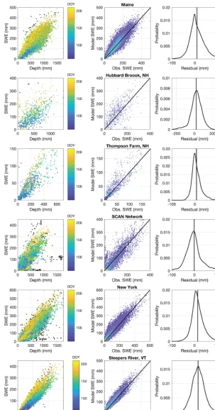
3.4 Results for northeastern United States
The regression equations in this study were developed us-ing a large collection of snow pillow sites in CONUS, AK, and BC. The snow pillow sites are limited to locations west of approximately 105◦W (Fig. 2a). By design, the data sets from the northeastern United States were left as an entirely independent validation set. These northeastern sites are ge-ographically distant from the training data sets, subject to a very different climate, largely use different methods (snow coring, with the exception of the SCAN network), and are generally at much lower elevations than the western sites, providing an interesting opportunity to test how robust the current model is.
Figure 12 graphically summarizes the data sets and the performance of the multivariable two-equation model of the
current study. The RMSE values are comparable to those found for the western stations, but, given the comparatively thinner snowpacks in the northeast, represent a larger relative error (Table 6). The bias of the model is consistently positive, in contrast to the western stations where the bias was negligi-ble. Note that Table 6 also includes results from the applica-tion of the other three models discussed. Sturm et al. (2010) cannot be applied to several of the data sets since their avail-able 1 km snow class data set cuts off at−71.6◦longitude. The current model and the Jonas et al. (2009) model perform better than the other two models, with the current model gen-erally outperforming the Jonas et al. (2009) model. The two data sets where the Jonas et al. (2009) model has a slightly better performance are the two smallest data sets (less than 1000 measurements; see Table 1).
3.5 Results for NRCS snow course/aerial marker data The NRCS snow course and aerial marker data were also left out of the model building process so they provide an addi-tional and completely independent comparison of the various models considered. Recall that these data come from snow course (coring measurements) and aerial surveys, which are different measurement methods than the snow pillows, which provided the data for construction of the current regression model. Figure 13 shows the aggregated snow course/aerial marker data set, along with the performance of the multivari-able two-equation model of the current study. Tmultivari-able 7 sum-marizes the results and demonstrates that the current model has the best performance.
4 Discussion
The results presented in this study show that the regression equation described by Eqs. (5), (7)–(8) is an improvement (lower bias and RMSE) over other widely used bulk den-sity equations. The key advantage is that the current method regresses in relevant parameters directly, rather than using discrete bins (for snow class, elevation, month of year, etc.), each with its own set of model coefficients. The comparison (Figs. 10–11; Table 4) to the model of Sturm et al. (2010) reveals a peculiar behavior of that model for the taiga snow class, with a large negative bias in the Sturm estimates. In-spection of the coefficients provided for that class (Table 3) shows that the model simply predicts thatρb=ρmax=0.217 for all conditions.
Table 6.Performance metrics for various models applied to the northeastern US data sets. Bold font is used to highlight the model with the best performance for each data set.
Data set name Multivariable, two-equation model Sturm et al. (2010) Jonas et al. (2009) Pistocchi (2015)
Bias RMSE Bias RMSE Bias RMSE Bias RMSE
(mm) (mm) (mm) (mm) (mm) (mm) (mm) (mm)
Maine Geological Survey, ME 13.1 34.0 – – 25.1 46.0 59.2 77.1
Hubbard Brook (Station 2), NH 21.8 66.6 34.2 76.9 19.4 65.4 52.0 90.8
Thompson Farm, NH 7.1 20.2 – – 5.6 19.9 20.4 32.3
NRCS SCAN −1.2 39.2 8.4 45.0 −2.8 40.6 23.4 56.9
Sleepers River, VT 14.4 28.2 36.5 48.9 20.4 33.5 55.8 67.1
New York Snow Survey 14.8 31.2 21.0 49.3 16.3 33.0 41.3 56.1
Table 7.Performance metrics for various models applied to the NRCS snow course and aerial marker data set. Bold font is used to highlight the model with the best performance.
Data set name Multivariable, Sturm et al. (2010) Jonas et al. (2009) Pistocchi (2015) two-equation model
Bias RMSE Bias RMSE Bias RMSE Bias RMSE
(mm) (mm) (mm) (mm) (mm) (mm) (mm) (mm)
NRCS snow course/aerial marker 0 59 −24 123 24 72 71 99
Figure 13.Results from application of the multivariable, two-equation model to the NRCS snow course/aerial marker data set. Panel(a) shows the SWE–hdata. Note that the black symbols are points removed during the data preprocessing stage. The remaining symbols are colored by DOY. Panel(b)shows a heat map of the model estimates of SWE against the observations of SWE with the 1:1 line included. Warmer colors indicate higher densities of points. Panel(c)shows the probability density function of the model residuals, with the vertical line indicating the mean error, or bias.
relation coefficients between SWE andh for each data set. It is unclear if this disparity in correlation is related to mea-surement methodology or is instead a signal-to-noise ratio issue. Comparing Figs. 4 and 12 shows the considerable dif-ference in snowpack depth between the western and north-eastern data sets. When the western data set is filtered to include only measurement pairs where h <1.5 m, the cor-relation coefficient is reduced to a value consistent with the northeast data sets. This suggests that the performance of the current (or other) regression model is not as good at shal-low snowpack depths. This is also suggested upon examina-tion of the time series of observedρb=SWE/ hfor a given season at a snow pillow site. Very early in the season, when
the depths are small, the density curve has a lot of variabil-ity. Later in the season, when depths are greater, the density curve becomes much smoother. Very late in the season, when depths are low again, the density curve becomes highly vari-able again.
ran-random and systematic errors in the paired SWE–hdata used to construct the regression model will lead to uncertainties in SWE values predicted by the model. As noted in the intro-duction, snow pillow errors in SWE estimates do not follow a simple pattern. Additionally, they are complicated by the fact that the errors are often computed by comparing snow pillow data to coring data, which itself is subject to error. Lacking quantitative information on the distribution of snow pillow errors, we are unable to quantify the uncertainty in the SWE estimates.
Another important consideration has to do with the un-certainty of depth measurements that the model is applied to. For context, one application of this study is to crowd-sourced, opportunistic snow depth measurements from pro-grams like the Community Snow Observations (CSO; Hill et al., 2018) project. In the CSO program, backcountry recreational users submit depth measurements, typically taken with an avalanche probe, using a smartphone in the field. The measurements are then converted to SWE esti-mates, which are assimilated into snowpack models. These depth measurements are “any time, any place” in con-trast to repeated measurements from the same location, like snow pillows or snow courses. Most avalanche probes have centimeter-scale graduated markings, so measurement pre-cision is not a major issue. A larger problem is the con-siderable variability in snowpack depth that can exist over short (meter-scale) distances. The variability of the Chugach avalanche probe measurements was assessed by taking the standard deviation of eight depth measurements per site. The average of this standard deviation over the sites was 22 cm and the average coefficient of variation (standard deviation normalized by the mean) over the sites was 15 %. This vari-ability is a function of the surface roughness of the underly-ing terrain, and also a function of wind redistribution of snow. Propagating this uncertainty through the regression equations yields a slightly higher (16 %) uncertainty in the SWE esti-mates. CSO participants can do three things to ensure that their recorded depth measurements are as representative as possible. First, avoid measurements in areas of significant wind scour or deposition. Second, avoid measurements in terrain likely to have significant surface roughness (rocks, fallen logs, etc.). Third, take several measurements and av-erage them.
tending back to the late 1800s. While many of the GHCN stations are confined to lower elevations with shallower snow depths, the broader network of quality-controlled snow depth data paired with daily GHCN temperature and precipitation measurements could potentially be used to reconstruct SWE in the eastern United States given additional model develop-ment and refinedevelop-ment.
5 Conclusions
We have developed a new, easy-to-use method for convert-ing snow depth measurements to snow water equivalent es-timates. The key difference between our approach and pre-vious approaches is that we directly regress in climatologi-cal variables in a continuous fashion, rather than a discrete one. Given the abundance of freely available climatological norms, a depth measurement tagged with coordinates (lati-tude and longi(lati-tude) and a time stamp is easily and immedi-ately converted into SWE.
We developed this model with data from paired SWE–h measurements from the western United States and British Columbia. The model was tested against entirely indepen-dent data (primarily snow course, some snow pillow) from the northeastern United States and was found to perform well, albeit with larger biases and root-mean-squared er-rors. The model was tested against other well-known regres-sion equations and was found to perform better. The model was also tested against a large data set of independent snow course and aerial marker measurements from western North America. For this second independent test, the current model outperformed the other models considered.
Data availability. Numerous online data sets were used for this project and were obtained from the following locations:
NRCS Snow Telemetry, https://www.wcc.nrcs.usda.gov/snow/ SNOTEL-wedata.html (last access: 1 August 2018);
NRCS Soil Climate Analysis Network, https://www.wcc.nrcs. usda.gov/scan/ (last access: 15 September 2018);
British Columbia Automated Snow Weather Sta-tions, https://www2.gov.bc.ca/gov/content/environment/ air-land-water/water/water-science-data/water-data-tools/ snow-survey-data/automated-snow-weather-station-data (last access: 1 October 2018);
Maine Cooperative Snow Survey, https://mgs-maine.opendata. arcgis.com/datasets/maine-snow-survey-data (last access: 15 October 2018);
New York Snow Survey, http://www.nrcc.cornell.edu/regional/ snowsurvey/snowsurvey.html (last access: 15 October 2018);
Sleepers River Research Watershed, snow data not available online; request data from contact at https://nh.water.usgs.gov/ project/sleepers/index.htm (last access: 30 October 2018);
Hubbard Brook Experimental Forest, https://hubbardbrook. org/d/hubbard-brook-data-catalog (last access: 30 October 2018);
Climatological Data, https://adaptwest.databasin.org/pages/ adaptwest-climatena (last access: 1 June 2019);
NRCS snow course/aerial marker data, https://wcc.sc.egov. usda.gov/reportGenerator/ (last access: 1 June 2019).
A MATLAB function for calculating SWE based on the results is this paper has been made publicly available at GitHub (https: //github.com/communitysnowobs/snowdensity).
Author contributions. JK contributed (acquisition, formatting, pre-liminary analysis) the Alaska and British Columbia data, JMH contributed the SNOTEL data, EAB and JK contributed the northeastern USA data, DFH contributed the western USA snow course/aerial marker data, RLC contributed the Chugach data. All authors contributed to the conception and direction of this study and to writing and editing of the manuscript. DFH conducted the regres-sion analysis and was the principal author of the manuscript.
Competing interests. The authors declare that they have no conflict of interest.
Acknowledgements. We thank Matthew Sturm, Adam Winstral, and the third anonymous referee for their careful and thoughtful reviews of this paper.
Financial support. This research has been supported by NASA (grant no. NNX17AG67A), CUAHSI (Pathfinder Fellowship grant), and the NSF (grant no. MSB-ECA 1802726).
Review statement. This paper was edited by Jürg Schweizer and re-viewed by Matthew Sturm, Adam Winstral, and one anonymous ref-eree.
References
Alford, D.: Density variations in alpine snow, J. Glaciol., 6, 495– 503, https://doi.org/10.3189/S0022143000019717, 1967. Avanzi, F., De Michele, C., and Ghezzi, A.: On the
per-formances of empirical regressions for the estimation of bulk snow density, Geogr. Fis. Din. Quat., 38, 105–112, https://doi.org/10.4461/GFDQ.2015.38.10, 2015.
Beaumont, R.: Mt. Hood pressure pillow snow gage, J. Appl. Meteorol., 4, 626–631, https://doi.org/10.1175/1520-0450(1965)004<0626:MHPPSG>2.0.CO;2, 1965.
Beaumont, R. and Work, R.: Snow sampling results from three samplers, Hydrolog. Sci. J., 8, 74–78, https://doi.org/10.1080/02626666309493359, 1963.
Burakowski, E. A., Wake, C. P., Stampone, M., and Dibb, J.: Putting the Capital “A” in CoCoRAHS: An Experimental Program to Measure Albedo using the Community Collaborative Rain Hail and Snow (CoCoRaHS) Network, Hydrol. Process., 27, 3024– 3034, https://doi.org/10.1002/hyp.9825, 2013.
Burakowski, E. A., Ollinger, S., Lepine, L., Schaaf, C. B., Wang, Z., Dibb, J. E., Hollinger, D. Y., Kim, J.-H., Erb, A., and Martin, M. E.: Spatial scaling of reflectance and surface albedo over a mixed-use, temperate forest landscape during snow-covered periods, Remote Sens. Environ., 158, 465–477, https://doi.org/10.1016/j.rse.2014.11.023, 2015.
Campbell, J., Ollinger, S., Flerchinger, G., Wicklein, H., Hayhoe, K., and Bailey, A.: Past and projected future changes in snow-pack and soil frost at the Hubbard Brook Experimental For-est, New Hampshire, USA, Hydrol. Process., 24, 2465–2480, https://doi.org/10.1002/hyp.7666, 2010.
Church, J. E.: Snow surveying: its principles and possibilities, Ge-ogr. Rev., 23, 529–563, https://doi.org/10.2307/209242, 1933. Church, J. E. and Marr, J. C.: Further improvement of
snow-survey apparatus, T. Am. Geophys. Un., 18, 607–617, https://doi.org/10.1029/TR018i002p00607, 1937.
Daly, C., Neilson, R., and Phillips, D.: A statistical-topographic model for mapping climatological pre-cipitation over mountainous terrain, J. Appl. Me-teorol., 33, 140–158, https://doi.org/10.1175/1520-0450(1994)033<0140:ASTMFM>2.0.CO;2, 1994.
De Maesschalck, R., Jouan-Rimbaud, D., and Massart, D.: The Mahalanobis distance, Chemometr. Intell. Lab., 50, 1–18, https://doi.org/10.1016/S0169-7439(99)00047-7, 2000. Dixon, D. and Boon, S.: Comparison of the SnowHydro sampler
with existing snow tube designs, Hydrol. Process., 26, 2555– 2562, https://doi.org/10.1002/hyp.9317, 2012.
52nd Annual Western Snow Conference, Sun Valley, ID, 188– 191, 17–19 April 1984.
Goodison, B., Glynn, J., Harvey, K., and Slater, J.: Snow Survey-ing in Canada: A Perspective, Can. Water Resour. J., 12, 27–42, https://doi.org/10.4296/cwrj1202027, 1987.
Hill, D. F., Wolken, G. J., Wikstrom Jones, K., Crumley, R., and Arendt, A.: Crowdsourcing snow depth data with citizen scien-tists, Eos, 99, https://doi.org/10.1029/2018EO108991, 2018. Johnson, J. and Marks, D.: The detection and correction of snow
water equivalent pressure sensor errors, Hydrol. Process., 18, 3513–3525, https://doi.org/10.1002/hyp.5795, 2004.
Johnson, J., Gelvin, A., Duvoy, P., Schaefer G., Poole, G., and Hor-ton, G.: Performance characteristics of a new electronic snow wa-ter equivalent sensor in different climates, Hydrol. Process., 29, 1418–1433, https://doi.org/10.1002/hyp.10211, 2015.
Jonas, T., Marty, C., and Magnusson, M.: Estimating the snow water equivalent from snow depth measurements, J. Hydrol., 378, 161– 167, https://doi.org/10.1016/j.jhydrol.2009.09.021, 2009. Leys, C., Klein, O., Dominicy, Y., and Ley, C.:
Detect-ing multivariate outliers: use a robust variant of the Ma-halanobis distance, J. Exp. Soc. Psychol., 74, 150–156, https://doi.org/10.1016/j.jesp.2017.09.011, 2018.
Liang, X., Lettermaier, D., Wood, E., and Burges, S.: A simple hy-drologically based model of land surface water and energy fluxes for general circulation models, J. Geophys. Res., 99, 14415– 14428, https://doi.org/10.1029/94JD00483, 1994.
Liston, G. and Elder, K.: A distributed snow evolution mod-eling system (SnowModel), J. Hydrometerol., 7, 1259–1276, https://doi.org/10.1175/JHM548.1, 2006.
Lundberg, A., Richardson-Naslund, C., and Andersson, C.: Snow density variations: consequences for ground penetrating radar, Hydrol. Process., 20, 1483–1495, https://doi.org/10.1002/hyp.5944, 2006.
McCreight, J. L. and Small, E. E.: Modeling bulk density and snow water equivalent using daily snow depth observations, The Cryosphere, 8, 521–536, https://doi.org/10.5194/tc-8-521-2014, 2014.
McKay, G. and Findlay, B.: Variation of snow resources with cli-mate and vegetation in Canada, Proceedings of the 39th Western Snow Conference, Billings, MT, 17–26, 20–22 April 1971. MCSS (Maine Cooperative Snow Survey): Maine Cooperative
Snow Survey Dataset, Maine Geological Survey, available at: https://www.maine.gov/dacf/mgs/hazards/snow_survey/, last ac-cess: 15 October 2018.
Meloysund, V., Leira, B., Hoiseth, K., and Liso, K.: Predicting snow density using meterological data, Meteorol. Appl., 14, 413–423, https://doi.org/10.1002/met.40, 2007.
Mote, P., Li, S., Letternaier, D., Xiao, M., and Engel, R.: Dramatic declines in snowpack in the western US, npj Climate and At-mospheric Science, 1, 1–6, https://doi.org/10.1038/s41612-018-0012-1, 2018.
NYSS (New York Snow Survey), NOAA, Northeast Regional Cli-mate Center, Cornell University, NY, USA, 2018.
Pagano, T., Garen, D., Perkins, T., and Pasteris, P.: Daily updat-ing of operational statistical seasonal water supply forecasts for the western U.S., J. Am. Water Resour. As., 45, 767–778, https://doi.org/10.1111/j.1752-1688.2009.00321.x, 2009. Painter, T., Berisford, D., Boardman, J., Bormann, K., Deems,
J., Gehrke, F., Hedrick, A., Joyce, M., Laidlaw, R., Marks, D., Mattmann, C., Mcgurk, B., Ramirez, P., Richardson, M., Skiles, S., Seidel, F., and Winstral, A.: The Airborne Snow Observatory: fusion of scanning lidar, imaging spectrometer, and physically-based modeling for mapping snow water equiv-alent and snow albedo, Remote Sens. Environ., 184, 139–152, https://doi.org/10.1016/j.rse.2016.06.018, 2016.
Pistocchi, A.: Simple estimation of snow density in an Alpine region, Journal of Hydrology: Regional Studies, 6, 82–89, https://doi.org/10.1016/j.ejrh.2016.03.004, 2016.
Rousseeuw, P.: Least Median of Squares Re-gression, J. Am. Stat. Assoc., 79, 871–880, https://doi.org/10.1080/01621459.1984.10477105, 1984. Ryan, W., Doesken, N., and Fassnacht, S.: Evaluation
of Ultrasonic Snow Depth Sensors for U.S. Snow Measurements, J. Atmos. Ocean. Tech., 25, 667–684, https://doi.org/10.1175/2007JTECHA947.1, 2008.
Schaefer, G., Cosh, M., and Jackson, T.: The USDA Natu-ral Resources Conservation Service Soil Climate Analysis Network (SCAN), J. Atmos. Ocean. Tech., 24, 2073–2077, https://doi.org/10.1175/2007JTECHA930.1, 2007.
Serreze, M., Clark, M., Armstrong, R., McGinnis, D., and Pulwarty, R.: Characteristics of the western United States snowpack from snowpack telemetry (SNOTEL) data, Water Resour. Res., 35, 2145–2160, https://doi.org/10.1029/1999WR900090, 1999. Shanley, J. and Chalmers, A.: The effect of frozen soil on
snowmelt runoff at Sleepers River, Vermont, Hydrol. Pro-cess., 13, 1843–1857, https://doi.org/10.1002/(SICI)1099-1085(199909)13:12/13<1843::AID-HYP879>3.0.CO;2-G, 1999.
Sturm, M., Holmgren, J., and Liston, G.: A seasonal snow cover classification system for local to global applica-tions, J. Climate, 8, 1261–1283, https://doi.org/10.1175/1520-0442(1995)008<1261:ASSCCS>2.0.CO;2, 1995.
data and climate classes, J. Hydrometeorol., 11, 1380–1394, https://doi.org/10.1175/2010JHM1202.1, 2010.
USACE (U.S. Army Corps of Engineers): Snow hydrology: Sum-mary report of the snow investigations of the North Pacific Di-vision, North Pacific DiDi-vision, Corps of Engineers, US Army, Portland, OR, USA, 437 pp., 1956.
USDA (U.S. Department of Agriculture): The History of Snow Sur-vey and Water Supply Forecasting, Interviews With U.S. Depart-ment of Agriculture Pioneers, edited By: Helms, D., Phillips, S., and Reich, P., Natural Resources Conservation Service, U.S. Department of Agriculture, Natural Resources Conservation Ser-vice, Washington D.C., USA, 2008.
USDA (U.S. Department of Agriculture): Snow Survey and Water Supply Forecasting. National Engineering Handbook Part 622, Water and Climate Center, Natural Resources Conservation Ser-vice, 2011.
Wang, T., Hamann, A., Spittlehouse, D. L., and Murdock, T.: Cli-mateWNA - High-Resolution Spatial Climate Data for West-ern North America, J. Appl. Meteorol. Clim., 51, 16–29, https://doi.org/10.1175/JAMC-D-11-043.1, 2012.
Wang, T., Hamann, A., Spittlehouse, D. L., and Carroll, C: Locally downscaled and spatially customizable climate data for historical and future periods for North America, PLoS One, 11, e0156720, https://doi.org/10.1371/journal.pone.0156720, 2016.