Hazard Rate Estimation Using Varying Kernel Function for Censored Data Type I

(1)

Baghdad Science Journal

Vol.16(3) Supplement 2019

DOI: http://dx.doi.org/10.21123/bsj.2019.16.3(Suppl.).0793

Hazard Rate Estimation Using Varying Kernel Function for Censored Data

Type I

Entsar Arebe Al.Doori

*

Eqbal Mhomod

Received 1/10/2018, Accepted 12/3/2019, Published 23/9/2019

This work is licensed under a Creative Commons Attribution 4.0 International License

.

Abstract:

In this research, several estimators concerning the estimation are introduced. These estimators are closely related to the hazard function by using one of the nonparametric methods namely the kernel function for censored data type with varying bandwidth and kernel boundary. Two types of bandwidth are used: local bandwidth and global bandwidth. Moreover, four types of boundary kernel are used namely: Rectangle, Epanechnikov, Biquadratic and Triquadratic and the proposed function was employed with all kernel functions. Two different simulation techniques are also used for two experiments to compare these estimators. In most of the cases, the results have proved that the local bandwidth is the best for all the types of the kernel boundary functions and suggested that the 2xRectangle and 2xEpanechnikov methods reflect the best results if compared to the other estimators.

Key words: Bandwidth, Censored Data, Hazard Rat, Kernel Function, Smoothing hazard rate

Introduction

:

Man’s need to continue his life in the best way is the first motive for the first studies and researches which are related to Survival Time. This takes into consideration the period of his survival when he suffers from certain disease (such as cancer). The nonparametric estimations concerning the hazard rate estimation of life time is a joint means of the statistics to prepare the censored survival data. The scientist Parzen(1962)(1) is the first one who has been highly concerned with the estimation by using varying kernel. It has been the weighting function and the kernel estimators have many uses such as (survival studies, epidemiology,

criminology and demography). The kernel

estimators are important as far as there are some problems when the stage of the end of the data is reached. This is referred to as the boundary effects. In fact, the boundary effects have been studied by some researchers such as Breslow and Day( 1987)(2) . The estimates of “the boundary areas”

curve did not show an area within the bandwidth of the endpoint. The application of unmodified kernel estimators causes meaningless estimation in the boundary areas near the endpoint. Recently, the researcher Salha in (2012)(3) estimated the hazard rate by using the Inverse Gaussian (IG) kernel and

College of Administration and Economic, University of Baghdad, Baghdad, Iraq.

*_{Corresponding} _author:

[email protected]

studied the nonparametric estimation of hazard rate by using kernel function. And Hind J. Kadhum& Iden H.Alkanani(2014)(4) using Survival estimation for singly type one centered sample based on generalized Rayleigh distribution. The aim of this paper is to compare several estimators of hazard rate estimation and show in the bandwidth. Two bandwidths are used namely global bandwidth and local bandwidth. Each one of them used four types of boundary kernel function: Rectangle, Epanechnikov, Biquadratic and Triquadratic ith a suggested method.

Materials and Methods (5,6):

Suppose that (t) represents life time variable with the rate of distribution and the hazard function is𝜆(𝑡)and this can be defined as follows (5):

𝜆(𝑡) =_{1−𝐹(𝑡)}𝑓(𝑡) , 𝑓𝑜𝑟 𝐹(𝑡) < 1 . . . (1)

Both of them are completed within the positive period of time. And the rate hazard means the specifications of the distribution:

Pr(𝑇 > 𝑡) = 𝑆(𝑡) = 𝑒𝑥𝑝 [− ∫ 𝜆(𝑠) 𝑡

0 𝑑𝑠]

(2)

Smoothing hazard rate for continuously observation data (7)

The estimation of hazard rate for continuously observation data is near the concept of density estimation. In order to know this, we replace the equation No (1) by the derivative of the cumulative hazard function:

Λ(𝑡) = ∫ 𝜆(𝑥)𝑑𝑥₀𝑡 . . . (2)

The estimation of hazard rate can be obtained from the increase of the estimation 𝚲(𝐭)

.From their part, the two scientists Watson and

Ledbetter (1964)(5) are the first who suggested and

studied the smoothing hazard rate by using the experimental cumulative hazard 𝚲𝒏(𝒕) according to

independent distributions i.i.d and the sample of the periods of hazard(𝛿_[𝑗] = 1) and they suggested the hazard estimation. The type of the convolution type hazard estimator (1)

𝜆̂𝑛(𝑡) = ∫ 𝛿₀𝑡 𝑛(𝑡 − 𝑥)𝑑Λ𝑛(𝑡) . . . (3)

Therefore{𝛿𝑛} is the sequence of smoothing

functions it is near Dirc delta – function when

𝑛 → ∞ The delta- function sequence is characterized by generality and it contains several types of smoothing and weighting function is one of them which has been used by Parzen (1962)(1) and as follows:

δn(x) = 1 bnk (

x bn)

Where 𝑏𝑛 is the bandwidth

The two scientists Watson and Leadbetter (1964)(5)

gave another estimation rate:𝜆̂𝑛(𝑡) =_1−𝐹̂𝑓̂𝑛 (𝑡) 𝑛 (𝑡) 𝑓̂_𝑛 is the density estimation of hazard density f and is an 𝐹̂_{𝑛 )} experimental estimation of the kernel hazard time distribution F.Both estimators have the same contrast but with different bias. The amount of convolution 𝜆̂𝑛(𝑡) is predominant because the

theoretical measures (mean square error available) outperformed the estimator of the ratio type𝜆̃𝑛(𝑡).Under the random control model the

current Ti time of the individual can be monitored by another random variable Ci and we will assume that:

1- 𝑇!, 𝑇2, … 𝑇𝑛is lifetime (time to failure) from

the observations of size (n) which are random distribution i.i.d identical and independent and it has the same distribution and it is positive with CDF continuous and cumulative hazard and continuous density hazard f.

(1 ) The convolution of the two kernels g , h can be defined in the following form:

(ℎ ∗ 𝑔)(𝑡) = ∫ 𝑔_−∞∞ (𝑡 − 𝜏)𝑑𝑡

2- 𝐶1, 𝐶2, … … 𝐶𝑛 refers to Censoring time. It

is a random distribution i.i.d. identical and independent and it has the same distribution. It is also positive with CDF joint cumulative hazard and continuous G density hazard.

3- The life time Xi and the censoring times Ci are independent and: 𝑋_𝑖= min (𝑇_𝑖, 𝐶_𝑖)

The 𝛿𝑖 = I{𝑥𝑖=𝑇𝑖}, 𝑖 = 1, … . 𝑛 progressively

arranged 𝑥 (𝑥 _(𝑖), 𝛿_(𝑖)) the sample is arranged according to 𝛿(𝑖) 𝑋(1) ≤ 𝑋(2)≤ ⋯ . ≤ 𝑋(𝑛) 𝑋𝑖 s

the indicator of censoring to 𝑋𝑖 and hazard

estimators can be obtained by smoothing estimators

𝚲𝒏(𝒕) Nelson-Aalen for the cumulative hazard

function and we suppose that:

𝑁_𝑛(𝑡) = ∑ I{𝑋≤𝑡,𝛿𝑖=1} 𝑛

𝑖=1

𝑌_𝑛(𝑡) = ∑ I_{{𝑋≥𝑡}} 𝑛

𝑖=1

The estimator 𝚲(. ) Nelson-Aalen in the analysis of observation data is defined by the following form:

𝚲_𝒏(𝒕) = ∫I{𝑦𝑛 (𝑠)>0} (𝑌)𝑛(𝑠) 𝑡

0

d𝑁_𝑛(s)

= ∑𝛿[𝑖]𝐼{𝑥(𝑖)≤𝑡} 𝑛 − 𝑖 + 1 𝑛

𝑖=1

… (4)

Provided that there is no link between the observations

Kernel Hazard Estimators(8):

To obtain the Kernel Hazard Estimators we choose the value:

δ_n(x) = 1 b_nk (

x − 𝑋(𝑖) b_n )

Where 𝑏_𝑛= 𝑏 𝑏𝑎𝑛𝑑𝑤𝑖𝑑𝑡ℎ . . . (5)

The equations No. (4) And (5) are replaced by the equation no. (3) By choosing kernel k and bandwidth 𝑏 = 𝑏𝑛 therefore we obtain the kernel

hazard estimator as follows:

𝜆̃(𝑥) = ∫1 𝑏k (

x − 𝑋

b_n ) Λ𝑛(𝑥)

=1 𝑏∑ k (

x − 𝑋_(𝑖) bn )

𝛿_(𝑖)

𝑛 − 𝑖 + 1… (6) 𝑛

𝑖=1

K is fixed kernel function. The bandwidth is of extreme importance and it organizes the differentiation between bias and contrast of the estimator in the equation (6). The small bandwidth

, , ,

(4)

(3)

causes little smoothing curve with small bias and great contrast if it is compared to big bandwidth. The characteristics of the hazard rate estimator function no.(5) has made use of by many researchers and we mention some of them Ramlau-Hansen (1983)(7), Taner and Wang (1983)(8) and we are able to get the characteristics of the adjacent consistency under certain assumptions are. Suppose that k is a round figure 𝑘 ≥ 0 and that 𝜆 is derivable and continuous for k of the times in the (O. R) period where R is the right endpoint so that L(R) < 1. The rate of the rounding of equation (6) is dependent on the degree of the core and the beam width. Application of the k-degree in the core selects an even number k = 2 the bias and the variation are respectively.

𝑏𝑖𝑎𝑠(𝜆̂_(𝑡)) = 𝑏𝑘_[𝜆(𝑘)_(𝑡)𝐵

𝑘+ 𝑜(1)] … (7)

𝑣𝑎𝑟 (𝜆̂(𝑡)) = 1 𝑛𝑏{

𝜆(𝑡)

[1 − 𝐹(𝑡)][1 − 𝐺(𝑡)]𝑣 + 𝑜(1)} … (8)

Where as

𝐵_𝑘 = (−1)𝑘

𝑘! ∫ 𝑘2_{𝐾(𝑥)𝑑𝑥} … (9) 𝑣 = ∫ 𝑘2_{(𝑥)𝑑𝑥 < ∞ … (10)}

By choosing Epanechnikov kernel as it is shown in the following equation:

𝑘(𝑥) = 0.075(1 − 𝑥2_{), −1 < 𝑥 < 1 … (11)}

The effect of bandwidth b and the differentiation between bias and variance is evident in the equations (8) (7) and for the parallel distribution, we assume that:𝑑 =

lim

𝑛→∞𝑛 𝑏2𝑘+1 Exist for some 0 ≤ 𝑑 ≤ ∞

(𝑛𝑏)12(𝜆̂(𝑡) − 𝜆(𝑡)) 𝐷

→ 𝑁 {𝑑12_𝜆(𝑘)(𝑥)𝐵_𝑥, 𝜆(𝑡)

[[1 − 𝐹(𝑡)][1 − 𝐺(𝑡)]]𝑣} … (12)

where D converge in distribution

Boundary Effects(9):

The unmodified kernel estimation is unreliable in the border area, whereas the bandwidth area is within larger or smaller observations to address the boundary effects of different data we

refer to by boundary kernel which can be used with he boundary area that is to say hazard function estimator with the different kernel functions and different bandwidth. The increase of bandwidth is different according to what is stated in order to realize the balance between the bias and the contrast thus reducing the error. e. The hazard estimator rate is defined with different degrees as it is shown in the following formula (3):

𝜆̂(𝑥) = 𝜆̂(𝑥, 𝑏(𝑥)) = 1

𝑏(𝑥)∑ 𝑘𝑥 𝑛

𝑖=1 (

x−𝑋(𝑖) 𝑏(𝑥) )

𝛿(𝑖)

𝑛−𝑖+1… (13)

The𝒃 = 𝒃(𝒙) represents the bandwidth and

𝑘 = 𝑘_𝑥 which is kernel and it depends upon the x point where the estimation has been calculated. We will discuss the choice of kernel 𝑘𝑥and bandwidth

b(x). The moment conditions in kernel boundary means that it carried the negative values and this will lead to negative hazard rate estimates as it is shown in the equation (No. 13) near endpoints. This might happen in the interior. In this case, we have to assume that: 𝜆̂(𝑥) = max (𝜆̂(𝑥), 0)

Bandwidth b(x) kernel kx chorice (9)(10):

The bandwidth in the kernel hazard function estimation can be fixed at all points (the global bandwidth b) or can be different in various points (local bandwidth). Normally, the global bandwidth is used to measure the density or to estimate the slope which is prevalent for its simplicity. The 𝐾𝑥

kernels

are:𝑘𝑥(𝑧) =

{

𝑘+(1, 𝑧) 𝑥𝜖𝐼 𝑘₊( 𝑥

𝑏(𝑥), 𝑧) 𝑥 ∈ 𝐵𝑙 𝑘₋(𝑅−𝑥

𝑏(𝑥), 𝑧) 𝑥 ∈ 𝐵𝑅

… (14)

𝐼 = {𝑥: 𝑏(𝑥) ≤ 𝑥 ≤ 𝑅 − 𝑏(𝑥)}= Is interior

(inside) and the effect of boundary is not calculated and𝐵𝑙 = {𝑥: 0 ≤ 𝑥 ≤ 𝑏(𝑥)} left boundary region 𝐵𝑅= {𝑥: 𝑅 − 𝑏(𝑥) < 𝑥 ≤ 𝑅}right boundary region 𝐾₊, 𝐾₋∶ [0,1] × [−1,1] → ℝ we notice that

𝐾₊(𝑞, . ) provide us in the time [-1, q] , 0 ≤ 𝑞 ≤

1 and 𝐾−(𝑞, . ) = 𝐾+(𝑞, . ) 0 ≤ 𝑞 < 1 . The

kernels𝐾₊(𝑞, . ) are called boundary kernels.

Table 1. The best forms of boundary kernels

𝜇

boundary kernel on [−1

,q

]

0 2

(1 + q)3[3((1 − q)x + 2((1 − q + q2]

Rectangle

1 12

(1 + 𝑞)4(x + 1)[𝑥(1 − 𝑞)(3𝑞2− 2𝑞 + 1/2]

Epanechnikov

2 15

(1 + 𝑞)5(𝑥 + 1)2(𝑞 − 𝑥 [(2𝑥) (5

1 − 𝑞

1 + 𝑞− 1) + (3𝑞 − 1) +

5(1 − 𝑞)2

1 + 𝑞 ]

Biquadratic

3 70

(1 + 𝑞)7(𝑥 + 1)3(𝑞 − 𝑥 [(2𝑥) (7

1 − 𝑞

1 + 𝑞− 1) + (3𝑞 − 1) +

7(1 − 𝑞)2

1 + 𝑞 ]

Triquadratic

… (13)

(4)

There are two familiar methods of showing the bandwidth which will be tackled later.

Local bandwidth (10) (11):

The display of the optimal local bandwidth at each point in the grid is obtained from the minimization of local MSE.

𝑀𝑆𝐸_𝑒𝑠𝑡(𝑥, 𝑏(𝑥)) = 𝑉̂(𝑥, 𝑏(𝑥)) + 𝐵̂2_{(𝑥, 𝑏(𝑥))}

. . . (15)

And the𝑣̂ ,𝛽̂ they are the variance bias respectively as follows:

𝑉̂(𝑥, 𝑏(𝑥)) =_{𝑛𝑏(𝑥)}1 ∫ 𝐾𝑥2(𝑦)_𝑙𝜆̂(𝑥−𝑏(𝑥)𝑦)_𝑛_{(𝑥−𝑏(𝑥)𝑦)}𝑑𝑦 …(16)

𝐵̂2(𝑥, 𝑏(𝑥)) = ∫ 𝜆̂(𝑥 − 𝑏(𝑥)𝑦)𝐾𝑥(𝑦)𝑑𝑦 − 𝜆̂(𝑥)

. . . (17)

𝐿_𝑛(𝑥) = 1 −_𝑛+11 ∑𝑛 𝐼_{{𝑋≤𝑥,𝛿}_𝑖_=1}

𝑖=1 …. (18)

The equation no. (18) is the empirical survival function of the uncensored observations and the equation Ln(x)=0 ,𝜆̂(. ) is pilot estimate to

𝜆 which has been formed by boundary correction and the fixed initial bandwidth bo is limited by the researcher. These estimations depend on the assumption of finite sample of bias and contrast which is from the convolution type derived by Muller and Wang (1990) (9). The minimizing bandwidth is:

𝑏̂(𝑥) = arg 𝑚𝑖𝑛𝑀𝑆𝐸_𝑒𝑠𝑡(𝑥, 𝑏) … (19)

Which has been referred as 𝜆̂(x,𝑏̂ (x)) hazard rate estimator in the equation (13) with the

bandwidth 𝑏̂ (𝑥).

Global bandwidth (9):

The global bandwidth is reflected itself in all the points of the grid. The optimal global bandwidth can be got from minimizing the integrated mean square error (IMSE)

𝐼𝑀𝑆𝐸𝑒𝑠𝑡(𝑏)

= ∫{𝑉̂(𝑥, 𝑏) + 𝐵̂2_{(𝑥, 𝑏)}dx … (20) .} 𝑅

0

𝒃̂ = 𝑎𝑟𝑔_𝑏𝐼𝑀𝑆𝐸_𝑒𝑠𝑡(𝑏) … (21)

B does not depend on x and the global bandwidth estimation

The following is the summary of hazard function estimation in algorithm:

Function estimation algorithm by using the local bandwidth (9):

The first step

We choose the kernel k+(q ,.) From the

timetable No. (1) About the methods of determining 𝜇𝜖{0,1,2, 3} and we recommend that

we choose the initial bandwidth bo depending on

the situation and it can be got in the following equation:

𝑏𝑛𝑑𝑤𝑖𝑑𝑡ℎ 𝑝𝑖𝑙𝑜𝑡 = 𝑅 8𝑛𝑧0.2

= (𝑚𝑎𝑥. 𝑡𝑖𝑚𝑒 − 𝑚𝑖𝑛. 𝑡𝑖𝑚𝑒)/(8𝑛𝑧0.2₎

nz is the number of uncensored observations. We suppose that the data is available during the period. [0, R] then we get the pilot estimators 𝜆(. )̂ according to the equation (13) and use𝑏(𝑥) = 𝑏𝑜

it does not depend on x and we get Kxaccording to the equation No. (14).

Instead of that we choose a parametric model and we fit it to the data by maximum likelihood method and the 𝜆̂_𝑝𝑎𝑟 refers to the fitting model.

The second step We choose an equidistant grid

and minimizing grid 𝑚1 from the points 𝑥̃𝑖 , 𝑖 = 1, … , 𝑚𝑖 between o and R the number m1 is the

grid point determine the calculated time to the largest expansion and it must not be very large. Then we choose the grid L bandwidth 𝑏̃𝑗, 𝑗 = 1, … , 𝐿𝑖 equidistant between b1 , b2 and we

recommend choosing:𝑏₁= 2𝑏₀/3 ,𝑏₂= 4𝑏₀ : for the points of the grid 𝑥̃_𝑖 and all the bandwidth 𝑏̃_𝑗 we calculate the variance and the bias 𝑣̂ and 𝛽̂ according to the equations (16) and (17) and we get the minimizers 𝑏̃(𝑥̃𝑖) for 𝑀𝑆𝐸𝑒𝑠𝑡(𝑥̃𝑖) according

to the equations No.(19) and the minimizing(𝑥̃𝑖)

for𝑏̌1… . . 𝑏̃𝐿

The third step we choose the equidistant grid and

estimation grid 𝑚₂ from the points 𝑥_𝑟, 𝑟 =

1, … . , 𝑚₂ between 0 and R which we desire the final hazard rate. We get the similar bandwidth

𝑏̂(𝑥) by smoothing the bandwidth 𝑏̂(𝑥̃𝑖) with

boundary - modified smoother by using the bandwidth𝑏̃₀ and 𝑏̃₀= 𝑏₀(𝑜𝑟 𝑏̃₀=3₂𝑏₀)

𝑏̂(𝑥_𝑟) =

∑𝑛𝑖=1𝑘𝑥,(𝑥𝑟_𝑏̃− 𝑥̃𝑖

𝑜 ) 𝑏̃(𝑥̃𝑖. ) ∑ 𝑘_𝑥(𝑥𝑟− 𝑥̃𝑖

𝑏̃𝑜 ) 𝑛

𝑖=1

… (22)

The fourth step To get the final hazard function

estimationℎ ̂(𝑥𝑟) from equation No.(13) by using:

Hazard function estimation algorithm by using global bandwidth (10):

The first step: Hazard function estimation

(5)

The second step we get the integrated mean square error (IMSE) according to the following

𝐼𝑀𝑆𝐸∗_(𝑏̃

𝑗) = ∑ 𝑀𝑆𝐸𝑒𝑠𝑡(𝑥̃𝑖𝑏̃𝑗) … (23) 𝑚𝑖

𝑖=1

equation:

𝑏̂ = 𝑚𝑖𝑛_𝑏̃_𝑗𝐼𝑀𝑆𝐸 ∗ (𝑏̃𝑗) . . . (24)

The third step: We choose the equidistant

estimation grid 𝑚₂ from the points 𝑥_𝑟, 𝑟 =

1, … . , 𝑚₂ as it is the case in the third step from the hazard function estimation algorithm by using local.

The fourth step: We calculate ℎ ̂ (𝑥_𝑟) according

to the equation No.(13) by using 𝑏(𝑥_𝑟) = 𝑏̂

The proposed function the researcher suggested

the following density function

𝑓(𝑥) = 2𝑥 , 0 ≤ 𝑥 ≤ 1 …. (25)

The empirical part(12):

The implementation of all the empirical simulation by using the programing language R (version 2.15.1 R 2012). This language is a large number of packages used in many different statistical fields. To carry out the experimentation of simulation different levels of factors are used and as follows:1-Size of different big medium and small samples :n = 30.60.80.100.2-The proposed density function in equation No. (25).3-The distributions used in this research Exponential distribution, Gamma distribution, Normal distribution, Log-normal distribution, Bimodal distribution. In order to determine the best method of distribution two criteria are used Average Mean Square Error (AMSE), Average Square Error (ASE), Average Maximum Deviation (AMXDV)

𝐴𝑀𝑆𝐸 = 1

1000 ∑ 𝐴𝑆𝐸𝑖 1000

𝐼=1

𝐴𝑆𝐸(𝜆) = 𝑚₂−1_{∑(𝜆(𝑥}

𝑟) − 𝜆̂(𝑥𝑟))2 𝑚2

𝑟=1

𝐴𝑀𝑋𝐷𝑉 = 1

1000∑ 𝑀𝑋𝐷𝑉𝑖 1000

𝐼=1

Plan of the performance of simulation experimentation

The programming language is a large increasing number of packages such as ‘dist’ package by which many distributions can be generated. From these packages we mention (muhaz package) by which it is possible to get the hazard function estimation of the first type and the kernel

with observation data m1=101 and m2=50 this experiment has been repeated (1000) times.

Perform the first simulation experiment

1- A. The sample 𝑥𝑖 ,1 ≤ 𝑖 ≤ 𝑛 has been

generated with gamma distribution G (5.1) with the parameter Fig. No 5 and the parameter 1.B. The variable 𝑐𝑖 ,1 ≤ 𝑖 ≤ 𝑛 has been generated from

the exponential distribution Exp(1/2.5) with the arithmetic mean 2.5.C. in A and B we find that the real hazard function takes the symbol hreal according to the equation No. (1).

2- Perform the global bandwidth algorithm by using muhaz function and we get the hazard function estimator and give it the symbol hest as it is in the equation No.(13) for four types of boundary kernel function which are:Rectangle, Epanechnikov, Biquadratic and Triquadratic which are explained in the table No. (1).We get AMSE for the four boundary kernels to find the difference with the square hest and hreal.

3-Perform the local bandwidth algorithm by using muhaz function and we get the hazard function estimator and give it the symbol hest as it is in the equation No.(13) for four types of boundary kernel function which are : Rectangle, Epanechnikov, Biquadratic and Triquadratic which are explained in the table No. (1).We get AMSE for the four boundary kernels to find the difference with the square hest and hreal.

Performing the proposed function experiment

1- A. The sample𝑥𝑖 ,1 ≤ 𝑖 ≤ 𝑛 has been

generated with the proposed density function x=2G which is the density function according to gamma distribution.

2- B. The variable C has been generated from the exponential distribution Exp(1/2.5) with the arithmetic mean 2.5

C. In A and B we find that the real hazard function takes the symbol hreal according to the equation No. (1).

3- Performing the global bandwidth algorithm by using muhaz function and we get the hazard function estimator and give it the symbol hest as it is in the equation No.(13) for four types of boundary kernel function which are : Rectangle, Epanechnikov, Biquadratic and Triquadratic which are explained in the table No. (1).We get AMSE for the four boundary kernels to find the difference with the square hest and hreal.

(6)

are explained in the table No. (1).We get AMSE for the four boundary kernels to find the difference with the square hest and hreal.

View and discussion of the results the first simulation experiment

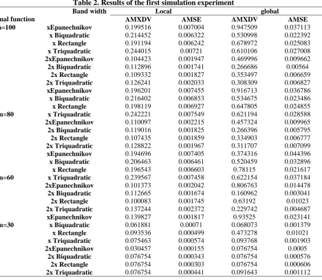
1- To show the local and global bandwidth and the size of the sample n=100,80 the lowest value of the standard AMSE in the proposed method 2xBiquadratic and the lowest value of the standard AMXDV in the proposed method are 2xEpanechnikov, 2xBiquadratic respectively, as it shown in Tables (1)and (2) and Fig. (1).

2- To show the local and global bandwidth and the size of the sample n=60 the lowest value of the standard AMSE in the proposed method 2xBiquadratic and the standard AMXDV in the proposed method is 2xRectangle, 2xBiquadratic respectively, as shown in Tables (1, 2) and Fig. (1).

3-To show the local and global bandwidth and the size of the sample n=30 the lowest value of the standard AMSE in the proposed method 2xEpanechnikov for two bandwidth and the lowest value of the standard AMXDV in the proposed method is 2x Epanechnikov,x Biquadratic respectively as shown in Table (1, 2)and Fig. (1). 4-The lowest value of the standard AMSE for the local and global bandwidth is in the proposed method 2xEpanechnikov and the size of the sample is n=30 as it is shown in Table (2).

5-The lowest value of the standard AMXDV for the local and global bandwidth is in the proposed method 2xEpanechnikov ,xBiquadratic respectively and the size of the sample is n=30 as it is shown in Table (2).

Table 2. Results of the first simulation experiment

global Local

Band width

Carnal function AMXDV AMSE AMXDV AMSE

(7)

n=100 l0cal global

n=80

n=60

n=30

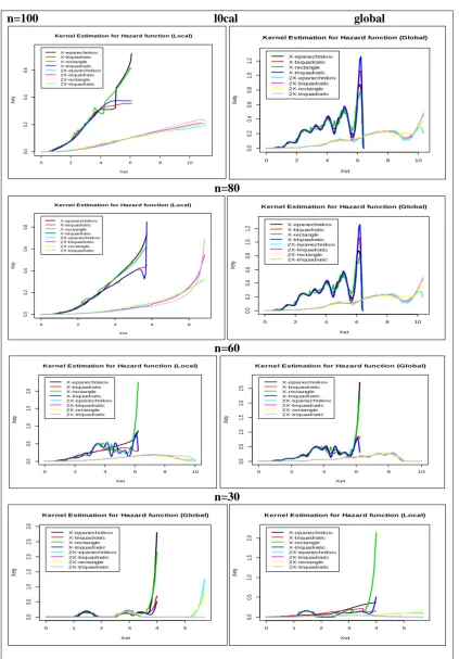
Figure 1. The estimation of the failure function represents the results of the first simulation experiment for two types of beam widths and different sample

Performing the second simulation experiment

1- A. The variable 𝑥𝑖 has been

generated from the density function of bimodal distribution which is used in (1992) by Kooperberg and Stone:

g is density function of normal algorithm

𝑓 =

0.8𝑔 + 0.2ℎ

distribution Lognormal, (O. ½) and h is the density function of normal distribution Normal (2,0.17) with arithmetic mean 2 with standard deviation 0.17.B. The variable 𝐶𝑖 has been

generated from the exponential distribution

0 2 4 6 8 10

0. 0 0. 2 0. 4 0. 6

Kernel Estimation for Hazard function (Local)

Xet X et y X-epanechnikov X-biquadratic X-rectangle X-triquadratic 2X-epanechnikov 2X-biquadratic 2X-rectangle 2X-triquadratic

0 2 4 6 8 10

0. 0 0. 2 0. 4 0. 6 0. 8 1. 0 1. 2

Kernel Estimation for Hazard function (Global)

0 2 4 6 8

0. 0 0. 2 0. 4 0. 6 0. 8

Xet Xe ty X-epanechnikov X-biquadratic X-rectangle X-triquadratic 2X-epanechnikov 2X-biquadratic 2X-rectangle 2X-triquadratic

0 2 4 6 8 10

0. 0 0. 2 0. 4 0. 6 0. 8 1. 0 1. 2

0 2 4 6 8 10

0. 0 0. 5 1. 0 1. 5 2. 0

0 2 4 6 8 10

0. 0 0. 5 1. 0 1. 5 2. 0 2. 5

0 1 2 3 4 5

0. 0 0. 5 1. 0 1. 5 2. 0 2. 5 3. 0

0 1 2 3 4 5

0. 0 0. 5 1. 0 1. 5 2. 0

(8)

Exp(1/2.5) with the arithmetic mean 2.5.C. In A and B we find that the real hazard function takes the symbol hreal according to the equation No. (1). 2- Performing the global bandwidth algorithm by using muhaz function and we get the hazard function estimator and give it the symbol hest as it is in the equation No.(13) for four types of boundary kernel function which are : Rectangle, Epanechnikov, Biquadratic and Triquadratic which are explained in the table No. (1).We get AMSE for the four boundary kernels to find the difference with the square hest and hreal.

3- Performing the local bandwidth algorithm by using muhaz function and we get the hazard function estimator and give it the symbol hest as it is in the equation No.(13) for four types of boundary kernel function which are : Rectangle, Epanechnikov, Biquadratic and Triquadratic which are explained in the table No. (1).We get AMSE for the four boundary kernels to find the difference with the square hest and hreal.

Performing the proposed function experiment

1- A. Generating the variable 𝑥𝑖 from the

proposed density function 𝑥 = 2𝑓and f is the bimodal distribution density function 𝑓 = 0.8𝑔 +

0.2ℎ

g is density function of normal algorithm distribution Lognormal ,

Lnorm (0.1/2) and h density function of normal distribution (2.0.17) with arithmetic mean 2 and standard deviation 0.17. B. The variable 𝐶𝑖 has

been generated from the exponential distribution Exp(1/2.5) with the arithmetic mean 2.5.

C. The paragraphs a and b we find the real hazard function with the symbol hreal according to the equation No. (1)

2- Performing the global bandwidth algorithm by using muhaz function and we get the hazard function estimator and give it the symbol hest as it is in the equation No.(13) for four types of boundary kernel function which are : Rectangle, Epanechnikov, Biquadratic and Triquadratic which are explained in the table No. (1).We get AMSE for the four boundary kernels to find the difference with the square hest and hreal.

3. Performing the local bandwidth algorithm by using muhaz function and we get the hazard function estimator and give it the symbol hest as it is in the equation No.(13) for four types of boundary kernel function which are : Rectangle,

Epanechnikov, Biquadratic and Triquadratic which are explained in the table No. (1).We get AMSE for the four boundary kernels to find the difference with the square hest and hreal.

View and discussion of the results of the second simulation experiment

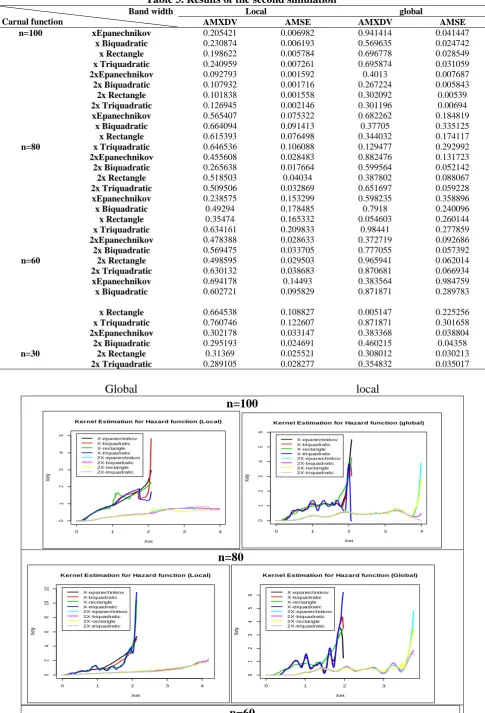
1- To show the local and global bandwidth and the size of the sample n=100 the lowest value of the standard AMSE in the proposed method 2xRectangle and of the standard AMXDV in the proposed Rectangle, 2xBiquadratic respectively as shown in Table (3) and Fig. (2).

2- To show the local and global bandwidth and the size of the sample n=80 the lowest value of the standard AMSE is in the proposed method

2xBiquadratic for two bandwidth and the lowest

value of the standard AMXDV is in the proposed method 2xBiquadratic , xTriquadratic respectively as it is shown in Table (3) and Fig. (2).

3- To show the local and global bandwidth and the size of the sample n=60 the lowest value of the standard AMSE is in proposed xEpanechnikov, 2xBiquadratic respectivly and of the standard

AMXDV is in the proposed method

2xEpanechnikov Rectangleg as it is shown in Table (3) and Fig. (2).

4- To show the local and global bandwidth and the size of the sample n=30 the lowest value of the standard AMSE is in the proposed method respectively and the lowest value of the standard AMXDV is in the proposed methodx Rectangle 2x Triquadratic respectively as it is shown in Table (3) and Fig. (2).

5- The lowest value of the standard AMSE for the local and global bandwidth is in the proposed method 2x Rectangle for two bandwidth and the size of the sample is n=100 as it is shown in Table (3).

6- The lowest value of the standard AMXDV for the local bandwidth is in the proposed method 2x Rectangle and the size of the sample is n=100 .and the lowest value of the standard AMXDV for the global bandwidth is in the proposed method x Rectangle and the size of the sample is n=30 as it is shown in Table (3).

(9)

Table 3. Results of the second simulation

global Local

Band width

Carnal function AMXDV AMSE AMXDV AMSE

0.041447 0.941414 0.006982 0.205421 xEpanechnikov n=100 n=80 n=60 n=30 0.024742 0.569635 0.006193 0.230874 Biquadratic x 0.028549 0.696778 0.005784 0.198622 Rectangle x 0.031059 0.695874 0.007261 0.240959 Triquadratic x 0.007687 0.4013 0.001592 0.092793 2xEpanechnikov 0.005843 0.267224 0.001716 0.107932 Biquadratic 2x 0.00539 0.302092 0.001558 0.101838 Rectangle 2x 0.00694 0.301196 0.002146 0.126945 Triquadratic 2x 0.184819 0.682262 0.075322 0.565407 xEpanechnikov 0.335125 0.37705 0.091413 0.664094 Biquadratic x 0.174117 0.344032 0.076498 0.615393 Rectangle x 0.292992 0.129477 0.106088 0.646536 Triquadratic x 0.131723 0.882476 0.028483 0.455608 2xEpanechnikov 0.052142 0.599564 0.017664 0.265638 Biquadratic 2x 0.088067 0.387802 0.04034 0.518503 Rectangle 2x 0.059228 0.651697 0.032869 0.509506 Triquadratic 2x 0.358896 0.598235 0.153299 0.238575 xEpanechnikov 0.240096 0.7918 0.178485 0.49294 Biquadratic x 0.260144 0.054603 0.165332 0.35474 Rectangle x 0.277859 0.98441 0.209833 0.634161 Triquadratic x 0.092686 0.372719 0.028633 0.478388 2xEpanechnikov 0.057392 0.777055 0.033705 0.569475 Biquadratic 2x 0.062014 0.965941 0.029503 0.498595 Rectangle 2x 0.066934 0.870681 0.038683 0.630132 Triquadratic 2x 0.984759 0.383564 0.14493 0.694178 xEpanechnikov 0.289783 0.871871 0.095829 0.602721 Biquadratic x 0.225256 0.005147 0.108827 0.664538 Rectangle x 0.301658 0.871871 0.122607 0.760746 Triquadratic x 0.038804 0.383368 0.033147 0.302178 2xEpanechnikov 0.04358 0.460215 0.024691 0.295193 Biquadratic 2x 0.030213 0.308012 0.025521 0.31369 Rectangle 2x 0.035017 0.354832 0.028277 0.289105 Triquadratic 2x

Global local

n=100

n=80

n=60

0 1 2 3 4

0 1 2 3 4 5

0 1 2 3 4

0 1 2 3 4 5 6

Kernel Estimation for Hazard function (global)

0 1 2 3 4

0 2 4 6 8 10 12

0 1 2 3

0 1 2 3 4 5 6

(10)

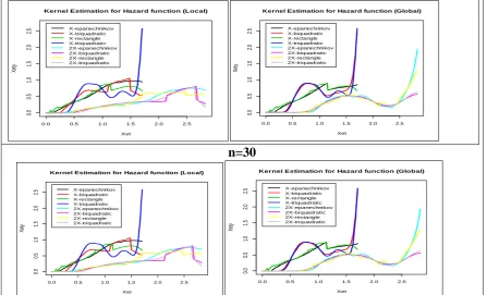
n=30

Figure 2. Estimation of the failure function represents the results of the second simulation experiment for two types of beam widths and different sample sizes

Conclusions:

1- The advantage of using the standard AMSE and for the two types of bandwidth for all the boundary of kernel function types and all the sizes of the samples except showing the global bandwidth in the x Biquadratic with the size of n=60.

2- The advantage of using the kernel function determines the proposed function 2x Epanechnikov with the local bandwidth and the size of the sample is n=30.

3- The advantage of using the kernel function determes the proposed function x Biquadratic with the local bandwidth and the size of the sample is n=30.

4- The advantage of using the kernel function determines the proposed function 2x Rectangle with the global bandwidth and the size of the sample is n=100.

5- The advantage of using the local bandwidth and the global bandwidth in reliability.

6- The increase of the value of AMSE with the increase of the sizes of the samples.

Conflicts of Interest: None.

References:

1. Parazen E . On Estimation of a Probability density Function and Mode, JMSA.1962;l(33):1065-1076.

2. Breslow N E, Day N E. The Design and Analysis of Studies. Statistical Methods in Cancer Research 1987;2;Oxford University Press.

3. Salha R.Hazard Rate function Estimation Using Inverse Gaussian Kernel .IUGNS. 2012;20;(1): 73-84. 4. Hind J K, Iden H Alkanani .Survival estimation for singly type one centered sample based on generalized Rayleigh distribution. Baghdad Sci.j.2014; 11 (2): 193-201. Publisher: Baghdad University.

5. Watson G S, Leadbetter, M R. Hazard analysis1. Biometrika.1964; 51:175-184.

6. Wang J L. Smoothing hazard rate .Encyclopedia of Biostatistics.2003; 2nd Edition; 7: 4986-4997.

7. Ramlau Hansen H. Smoothing Counting process Intensities by means of kernel function. Ann. statist.1983; 11(2): 453-466.

8. Tanner M A, Wong W H. The estimation of the hazard function from randomly censored data by the kernel method. Ann.Statit.1983; 1: 989-993.

9. Müller HG Wang J L .Hazard rate estimation under random censoring with varying kernels and bandwidths.Biometrics.1994; 50 (1): 61-76.

10. Müller HG, Wang JL. Locally adaptive hazard smoothing. Probab. Theory Related Fields.1990; 85; 523-538.

11. Philip Sieger, Eirini. Tatsi

.

nonparametric estimation of the hazard function .Goeth UniversityFrankfurt Fculty of Economicsand business administration. 2010, September 15.

12. Kooperberg C, Stone C J. Logspline density estimation for censored data. J. comput. Graph. Statist.1992; 1: 301-328.

0.0 0.5 1.0 1.5 2.0 2.5

0.

0

0.

5

1.

0

1.

5

2.

0

2.

5

Xet

Xe

ty

X-epanechnikov X-biquadratic X-rectangle X-triquadratic 2X-epanechnikov 2X-biquadratic 2X-rectangle 2X-triquadratic

0.0 0.5 1.0 1.5 2.0 2.5

0.

0

0.

5

1.

0

1.

5

2.

0

2.

5

Xet

Xe

ty

0.0 0.5 1.0 1.5 2.0 2.5

0.

0

0.

5

1.

0

1.

5

2.

0

2.

5

Xet

Xe

ty

0.0 0.5 1.0 1.5 2.0 2.5

0.

0

0.

5

1.

0

1.

5

2.

0

2.

5

Xet

Xe

ty

(11)

لولاا عونلا نم ةبقارم تانايبل ةفلتخم ةيبل لاود لامعتساب لشفلا ةلاد ريدقت

معدف يبيرع راصتنا

دومحم لابقا

مسق ءاصحلاا ، داصتقلااو ةرادلاا ةيلك

،

قارعلا ،دادغب ،دادغب ةعماج

ةصلاخلا

:

تانايبل ةيبللا لاودلا يهو ةيملعملالا قرطلا ىدحإ لامعتساب لشفلا ةلاد ريدقتب ةصاخلا تاردقملا نم ددع ميدقت مت ثحبلا اذه يف

ةيبللا لاودلاو مزحلا ضرع نم ةفلتخم عاونلأ لولأا عونلا نم ةبقارم مزحلا ضرع نم نيعون لمعتسا ثيح ، دودحلا

ةمزحلا ضرع

لماشلا ةيبل لاود عبرلاو لاود عبرلاو gobal bandwidth

يعضوملا ةمزحلا ضرعو local bandwidth

Rectangle,

Epanechnikov, Biquadratic and Triquadratic ةيبللا لاودلا يف ةحرتقم ةلاد فيضوت كلذكو

نيتفلتخم ةاكاحم نيتبرجتلو ةفاك

تاردقملا كلت ةنراقمل يعضوملا ةمزحلا ضرع بولسأ ةيلضفأ جئاتنلا تتبثأ دقو

local bandwidth دودحلا ةيبللا لاودلا عاونأ عيمجل

دودحلا ةيبللا لاودلا لامعتسإ ةيلضفاو . ةحرتقملا ةلادلل

Rectangle 2x

ةلادلاو 2xEpanechnikov

لا رثكلا . ةماقملا براجت

:ةيحاتفملا تاملكلا