Effects of CO 2, continental distribution, topography and vegetation changes on the climate at the Middle Miocene: a model study

(1)

Clim. Past, 6, 675–694, 2010 www.clim-past.net/6/675/2010/ doi:10.5194/cp-6-675-2010

Climate

of the Past

Effects of CO

2

, continental distribution, topography and vegetation

changes on the climate at the Middle Miocene: a model study

A.-J. Henrot1, L. François2, E. Favre2, M. Butzin3, M. Ouberdous2, and G. Munhoven1 1_{Laboratory of Atmospheric and Planetary Physics, University of Liège, Liège, Belgium}

2_{Unité de Modélisation du Climat et des Cycles Biogéochimiques, University of Liège, Liège, Belgium} 3_{MARUM – Center for Marine Environmental Sciences, University of Bremen, Bremen, Germany} Received: 16 March 2010 – Published in Clim. Past Discuss.: 14 April 2010

Revised: 27 September 2010 – Accepted: 18 October 2010 – Published: 21 October 2010

Abstract. The Middle Miocene was one of the last warm

pe-riods of the Neogene, culminating with the Middle Miocene Climatic Optimum (MMCO, approximatively 17–15 Ma). Several proxy-based reconstructions support warmer and more humid climate during the MMCO. The mechanisms responsible for the warmer climate at the MMCO and par-ticularly the role of the atmospheric carbon dioxide are still highly debated. Here we carried out a series of sensitivity ex-periments with the model of intermediate complexity Planet Simulator, investigating the contributions of the absence of ice on the continents, the opening of the Central American and Eastern Tethys Seaways, the lowering of the topography on land, the effect of various atmospheric CO2 concentra-tions and the vegetation feedback.

Our results show that a higher than present-day CO2 con-centration is necessary to generate a warmer climate at all lat-itudes at the Middle Miocene, in agreement with the terres-trial proxy reconstructions which suggest high atmospheric CO2concentrations at the MMCO. Nevertheless, the changes in sea-surface conditions, the lowering of the topography on land and the vegetation feedback also produce significant local warming that may, locally, even be stronger than the CO2 induced temperature increases. The lowering of the topography leads to a more zonal atmospheric circulation and allows the westerly flow to continue over the lowered Plateaus at mid-latitudes. The reduced height of the Tibetan Plateau notably prevents the development of a monsoon-like circulation, whereas the reduction of elevations of the North American and European reliefs strongly increases precipita-tion from northwestern to eastern Europe.

Correspondence to: A.-J. Henrot

([email protected])

The changes in vegetation cover contribute to maintain and even to intensify the warm and humid conditions pro-duced by the other factors, suggesting that the vegetation-climate interactions could help to improve the model-data comparison.

1 Introduction

(2)

676 A.-J. Henrot et al.: Middle Miocene climate modelling experiments the reconstructions of K¨urschner et al. (2008) based on leaf

stomatal indices indicate much higher MMCO CO2 levels between 300 and 600 ppmv. Reconstructions based on pa-leosoil analysis indicate an even higher CO2 concentration of 850 ppmv (Retallack, 2009). However, CO2 concentra-tions reconstructed on the basis of planktonic foraminiferal

δ18O temperature reconstructions are possibly biased due to estimates of ice volume or diagenesis (Pagani et al., 2010, Supplement). Alkenone-based temperature reconstructions could possibly lead to higher CO2 concentration estimates for the Miocene (Pagani et al., 2010, Supplement).

The reconfiguration of inter-oceanic passages which sig-nificantly influences the ocean circulation may also have contributed to the MMCO climate (Bice et al., 2000; Von der Heydt and Dijkstra, 2008). The Central Amer-ican Seaway and Eastern Tethys Seaway were notably open during the Middle Miocene (Herold et al., 2008), leading to significantly different ocean circulation patterns (Von der Heydt and Dijkstra, 2006).

Geological processes such as mountain uplift may also affect the atmospheric circulation and precipitation patterns (Gregory-Wodzicki, 2000; Harris, 2006). Although the po-sitions of the continents were close to modern, most of the higher orogens got elevated during the Miocene, such as the Himalayas and the Tibetan Plateau (Currie et al., 2005; Harris, 2006), the Central Andes (Gregory-Wodzicki, 2000) as well as the Alps (Kuhlemann et al., 2006). Topography was therefore generally lower at the Middle Miocene than at present-day (Herold et al., 2008).

Finally it should also be noticed that the warm climate pre-vailing during the Middle Miocene led to vegetation changes. Broadleaved evergreen forests appear to have extended as far north as 45◦_{N in North America and 52}◦_{N in}

Eu-rope (Utescher et al., 2000). Such a change in the vegeta-tion cover may have led to significant impacts on climate (Dutton and Barron, 1997).

Up to now, only a few climate model simulations have been performed for the Middle Miocene. Von der Heydt and Dijkstra (2006) used an AOGCM (Community Climate System Model (CCSM v.1.4)) to study the effect of ocean gateways on global ocean circulation patterns in the Late Oligocene to Early Miocene. Their results indicated that the different configuration of the ocean gateways may have sig-nificantly affected the global thermohaline circulation in the Miocene. However, they did not assess any topographic nor vegetation effect. They prescribed a flat land with a constant elevation of 350 m and a zonally constant vegetation distribu-tion. The ocean model that they used furthermore had a flat bottom ocean at 5000 m depth. More recent climate mod-elling sensitivity experiments have particularly focused on the sensitivity of the Miocene climate to various atmospheric CO2 concentrations using atmospheric models (Tong et al., 2009; You et al., 2009). Tong et al. (2009) used the NCAR Community Atmosphere Model (CAM v.3.1) and Commu-nity Land Model (CLM v.3.0) coupled to a slab ocean to

examine the sensitivity of the Middle Miocene climate to successive quasi-doubling of atmospheric CO2concentration (180 355 and 700 ppmv). You et al. (2009) used the same NCAR models coupled to a slab model to analyse the sen-sitivity of the MMCO climate to varying ocean heat fluxes derived from palaeo sea surface temperatures and successive quasi-doubling of atmospheric CO2concentrations (180 355 and 700 ppmv) and compared their global temperature esti-mations to available proxy data. Both studies required higher than present-day CO2 concentrations to produce a warmer climate at the MMCO. However, Tong et al. (2009) and You et al. (2009) also found that the sole increase of CO2 is not sufficient to produce the MMCO warming inferred from proxy-data. Finally, Herold et al. (2009) tested the impact of altered Andean and Tibetan Plateau elevations on the MMCO climate again with the same NCAR models, and fixed sea surface temperatures. Herold et al. (2009) indicated that the reduction of the Tibetan Plateau and Andes elevations signif-icantly affects local temperatures. However, they also con-cluded that topography alone could not be a significant factor in reconciling the warm MMCO climate and the CO2 con-centration estimates.

The objective of the present study is to examine the con-tribution of several boundary condition changes to the warm MMCO climate and particularly to discuss the contribution of the vegetation feedback as a potential alternative mech-anism to the large increase of CO2 required by the mod-els to produce a warmer climate at the MMCO. Therefore, we performed a series of simulation experiments with the Planet Simulator, where we have assessed the effects of the absence of ice on the continents, the opening of the Cen-tral American and Eastern Tethys Seaways, the lowering of the topography on land and the effect of various atmospheric CO2 concentrations. We reconstructed the vegetation dis-tribution for the Middle Miocene in response to the MMCO boundary conditions previously cited, using the CARAIB dy-namic vegetation model. We then forced the Planet Simula-tor with the reconstructed Middle Miocene vegetation distri-bution to assess the vegetation feedback in response to the Middle Miocene simulated climate. We first describe our model setup (Sect. 2.1) and examine the response of surface climate (temperature, precipitation and low level winds) to the different forcings (Sect. 3). Finally, we discuss the con-tribution of the factors on the Middle Miocene climate, fo-cusing in particular on the contribution of vegetation cover changes (Sect. 4).

2 Model and experimental design

(3)

A.-J. Henrot et al.: Middle Miocene climate modelling experiments 677 different past periods (Romanova et al., 2006; Henrot et al.,

2009), notably the late Miocene (Micheels et al., 2009b). The model has proven usefulness in the comparison to proxy data (Henrot et al., 2009; Micheels et al., 2009a). The Planet Sim-ulator present-day climate compares fairly well to ERA-40 reanalysis although it is affected by two major climatological biases: (1) a cold bias at high latitudes in winter of the hemi-sphere and (2) a global overestimation of the surface evapo-ration (Haberkorn et al., 2009). The central component of the Planet Simulator is PUMA-2, a spectral GCM with triangu-lar truncation, based upon the Portable University Model of the Atmosphere, PUMA (Fraedrich et al., 1998). PUMA-2 solves the moist primitive equations, representing the con-servation of momentum, mass and energy, onσ coordinates in the vertical. It also includes boundary layer, precipita-tion, interactive clouds and radiation parametrizations. For the present study, we configured it to use a T42 truncation and ten vertical equally spacedσ levels. The model atmo-sphere is coupled to a 50 m deep mixed-layer ocean, a ther-modynamic sea-ice and a land surface and soil model.

Sea surface temperatures are computed from the net at-mospheric heat flux at the surface. The transport of heat by oceanic surface currents is represented by an additional dis-tribution of heat sources and sinks that is prescribed within the mixed-layer and the sea-ice and that varies monthly and spatially. Their distributions for the preindustrial period and the Middle Miocene were determined from preindustrial and Miocene experiments respectively, where sea surface tem-perature and sea-ice distributions were obtained from simu-lations with an updated version of the Hamburg LSG circula-tion model (developed by Maier-Reimer et al., 1993) (Butzin et al., 2010). This procedure allows the model to respond with a larger sensitivity to boundary condition changes than with prescribed sea-surface temperatures.

The land surface and soil models calculate the surface tem-peratures from a linearized energy balance equation and pre-dict soil moisture on the basis of a simple bucket model. The influence of vegetation is represented by background albedo, roughness length and rooting depth. Their annual distribu-tions are prescribed, and albedo may only change in grid-cells where snow is present. The distributions of surface albedo, roughness length and rooting depth were obtained from a preindustrial run and a Middle Miocene run of the dynamic vegetation model CARAIB (CARbon Assimilation In the Biosphere) (Otto et al., 2002; Franc¸ois et al., 2006; Laurent et al., 2008). CARAIB calculates the carbon fluxes between the atmosphere and the terrestrial biosphere and de-duces the evolution of carbon pools, together with the rel-ative abundances of a series of plant functional types. Its different modules respectively focus on the hydrological cy-cle, photosynthesis and stomatal regulation, carbon alloca-tion and biomass growth, heterotrophic respiraalloca-tion and lit-ter and soil carbon, and the distribution of the model plant types, as a function of productivity. Here we use a classifica-tion including 15 Plant Funcclassifica-tional Types (PFTs), described

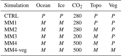
Table 1. Description of the simulation experiments. P refers to

preindustrial conditions andMrefers to Miocene conditions. Each one of the five columns corresponds to each of the five modified boundary conditions: ocean heat transfer, ice-sheet cover, atmo-spheric CO2concentration (in ppmv), topography and vegetation

cover

Simulation Ocean Ice CO2 Topo Veg

CTRL P P 280 P P

MM1 M M 280 P P

MM2 M M 280 M P

MM3 M M 200 M P

MM4 M M 500 M P

MM4-veg M M 500 M M

in Utescher et al. (2007) and Galy et al. (2008). Model de-rived PFT assemblages can be translated into biomes to pro-duce vegetation maps. The inputs of the model are meteo-rological variables, taken from meteometeo-rological databases or GCM simulation experiments.

2.1 Experimental setup

In this work we examine the potential contribution of sev-eral boundary condition forcings to the MMCO. We there-fore perform a series of five sensitivity experiments where we have assessed the effects of the absence of ice on the continents, the opening of the Central American and East-ern Tethys Seaways, the lowering of the topography on land, of various atmospheric CO2concentrations and the effect of vegetation cover changes on climate (through surface albedo, roughness length and rooting depth, i. e., bucket size) in re-sponse to the Middle Miocene simulated climate. Table 1 lists the boundary condition changes applied for the series of experiments. The control experiment (CTRL) does not con-sider any of the changes and corresponds to a preindustrial state. All experiments have been run for 50 years and the results shown in Sect. 3 are means over the last 20 years of simulation, allowing 30 years for the model to equilibrate.

2.1.1 Land ice

(4)

678 A.-J. Henrot et al.: Middle Miocene climate modelling experiments

2.1.2 Ocean and sea-ice

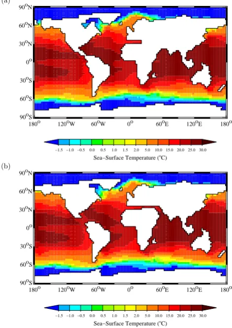
There is currently no global proxy-based SST reconstruc-tion available for the MMCO that could be directly used with GCMs. Furthermore several biases towards no-tably colder temperatures have been detected in the oxy-gen isotope palaeo SST estimates (Pearson et al., 2007). Williams et al. (2005) also suggested that the Miocene trop-ical sea surface temperatures may be underestimated in the current reconstructions, due notably to diagenesis. We there-fore preferred to use as initial conditions over ocean grid points sea-surface temperature and sea-ice distributions de-rived from simulations of the updated Hamburg LSG cir-culation model, which includes a simple atmospheric en-ergy balance model permitting that the LSG SSTs freely adjust to ocean circulation changes (Butzin et al., 2010). Butzin et al. (2010) performed several simulation experi-ments to assess the sensitivity of benthic carbon isotope records to various seaway configurations and sea-ice sce-narii. In this work, we use as initial oceanic conditions for all the Miocene simulation experiments the sea-surface temper-ature and sea-ice distributions from one LSG simulation fea-turing open Central American and Eastern Tethys Seaways, a filled Hudson Bay and a closed Bering Strait, according to Gladenkov et al. (2002), a fixed atmospheric CO2 con-centration of 282 ppmv, and sea ice extent around 90% of the present-day value. Preindustrial LSG results were also used to derive the preindustrial sea-surface temperature and sea-ice distributions for the control run of our series. The LSG Miocene run’s spinup is 10 000 years long and the LSG sea-surface temperatures and sea-ice cover used here as ini-tial conditions are means over the last 50 years of simula-tion. The LSG sea-surface temperature and sea-ice cover for the preindustrial and the Miocene are shown in Fig. 1. In the Miocene LSG simulation, the opening of the Cen-tral American Seaway freshened the upper part of North At-lantic while salinities increased in the other oceans. The Meridional Overturning Circulation (MOC) in the Atlantic Ocean weakened. As a consequence, the upper North At-lantic got cooler and the South AtAt-lantic warmer. The Eastern Tethys Seaway weakly impacted on Indian Ocean heat trans-port (Butzin et al., 2010). The impact of a closed Bering Strait is more convoluted (the Bering Strait first opened in the Late Miocene at about 5.4–5.3 Ma, Gladenkov et al., 2002). A closed Bering Strait may reinforce the impact of the open Central American Seaway. An open Bering Strait in a Late Miocene LSG sensitivity experiment mitigated the effect of the open Central American Seaway, because of a freshwater export from the Arctic Ocean into the North Pacific via the Bering Strait (unpublished results). The water flux through the open Bering Strait in the Miocene LSG experiment is op-posite to the present-day water flux from the North Pacific to the Arctic Ocean, which is in line with results of fully cou-pled freshwater perturbation experiments under present-day conditions (Okumura et al., 2009).

(a)

180o 120oW 60oW 0o 60oE 120oE 180o 90oS

60oS 30oS 0o 30oN 60oN 90oN

−1.5 −1.0 −0.5 0.0 0.5 1.0 1.5 2.0 5.0 10.0 15.0 20.0 25.0 30.0 Sea−Surface Temperature (o

C)

(b)

180o 120oW 60oW 0o 60oE 120oE 180o 90oS

C)

(a)

180o 120oW 60oW 0o 60oE 120oE 180o 90oS

C)

(b)

180o 120oW 60oW 0o 60oE 120oE 180o 90oS

−1.5 −1.0 −0.5 0.0 0.5 1.0 1.5 2.0 5.0 10.0 15.0 20.0 25.0 30.0 Sea−Surface Temperature (o_C)

Fig. 1. Initial sea-surface temperatures for (a) the CTRL experiment

and (b) the Miocene experiments. Grid elements with a temperature below−1.5◦C are covered by sea-ice.

(5)

A.-J. Henrot et al.: Middle Miocene climate modelling experiments 679

(a)

180o 120oW 60oW 0o 60oE 120oE 180o 90oS

−150−100 −75 −50 −25 −15 −10 −5 0 5 10 15 25 50 75 100 150 Ocean heat flux (W/m*m)

(b)

180o 120oW 60oW 0o 60oE 120oE 180o 90oS

(a)

180o 120oW 60oW 0o 60oE 120oE 180o 90oS

(b)

180o 120oW 60oW 0o 60oE 120oE 180o 90oS

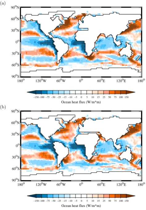
Fig. 2. Oceanic surface heat transfer for (a) the CTRL configuration

and (b) the Miocene configuration. Positive values indicate a net transfer of heat from the ocean to the atmosphere.

Seaway, but an increase of the heat transfer to the South At-lantic. However, besides the reorganization of heat transfer in the Atlantic Ocean, the distribution of the surface heat fluxes at the Miocene does not differ much from the preindustrial distribution.

2.1.3 Land-sea distribution and topography

The use of LSG sea-surface temperatures as initial oceanic conditions imposed us to stick to the land-sea distribution and corresponding topography prescribed in the LSG exper-iments (Butzin et al., 2010). The control experiment was therefore forced with the present-day LSG land-sea mask and topography, whereas the Miocene experiments were forced with the Miocene LSG land-sea mask which takes into ac-count an open Central American Seaway, an open Eastern Tethys Seaway, a filled Hudson Bay and a closed Bering Strait as stated above (see Fig. 3). However, the Miocene LSG simulations consider a present-day topography on land. It is thought that elevation on land was globally lower dur-ing the Miocene (Ruddiman, 1997; Harris, 2006;

Gregory-(a)

180o 120oW 60oW 0o 60oE 120oE 180o 90oS

50 500 1000 1500 2000 2500 3000 3500 4000 4500 5000 Topography (m)

(b)

180o 120oW 60oW 0o 60oE 120oE 180o 90oS

50 500 1000 1500 2000 2500 3000 3500 4000 4500 5000 Topography (m)

(a)

180o 120oW 60oW 0o 60oE 120oE 180o 90oS

50 500 1000 1500 2000 2500 3000 3500 4000 4500 5000 Topography (m)

(b)

180o 120oW 60oW 0o 60oE 120oE 180o 90oS

50 500 1000 1500 2000 2500 3000 3500 4000 4500 5000 Topography (m)

Fig. 3. Land-sea mask and topography on land for (a) the CTRL

configuration and (b) the Miocene configuration.

Wodzicki, 2000). We therefore applied the algorithm de-scribed in Kutzbach et al. (1989) in order to reconstruct a topography approximatively at half-height of its modern elevation.

h = 400 m+(h0−400 m)/2 whereh0≥400 m

(6)

680 A.-J. Henrot et al.: Middle Miocene climate modelling experiments the ones reported in Herold et al. (2008). However, the

max-imum elevation of the Tibetan Plateau is limited to 3500 m in our reconstruction, whereas Herold et al. (2008) constrained it to 4700 m. On the contrary, the Andes are around 500 m higher in our Miocene topography. Nevertheless, the dif-ferences between both topography reconstructions remain within the paleoelevation data errors for the Tibetan Plateau (Currie et al., 2005; Wang et al., 2006) and the Andes (Gregory-Wodzicki, 2000).

2.1.4 Vegetation cover

Surface boundary condition parameters controlled by the vegetation cover (surface albedo, roughness length and root-ing depth) have been derived from equilibrium runs of the CARAIB model. The surface albedo, roughness length and rooting depth of the land grid-cells are calculated from the PFT abundances and specific albedo, roughness length and rooting depth values attributed to each PFT. To obtain the preindustrial vegetation parameters, we performed an equi-librium run of CARAIB, forced with 280 ppmv of CO2and the climatology of New et al. (2002). All of the experi-ments were forced with the preindustrial vegetation parame-ters except for experiment veg. In experiment MM4-veg, the vegetation parameters were replaced by their Mid-dle Miocene distributions derived from an equilibrium run of CARAIB forced with 500 ppmv of CO2 in the atmosphere and the climate from the experiment MM4, which is the warmest and most humid of the series and in best agree-ment with proxy-based climate reconstructions (see Sect. 4). We used the anomalies of the GCM climatic fields between the Middle Miocene (experiment MM4) and the preindustrial (experiment CTRL), added to the climatology of New et al. (2002), as climatic inputs for the Middle Miocene CARAIB simulation, following the approach described in Otto et al. (2002). The vegetation parameters of the emerging land-points from the Miocene land-sea distribution were extrap-olated from the vegetation parameters of the nearby land-points, using an inverse distance weighted average proce-dure.

2.1.5 Atmospheric CO2concentration

We forced our simulations with various atmospheric CO2 concentrations. The control experiment, as well as the first Miocene simulation experiments MM1 and MM2 used a preindustrial CO2level of 280 ppmv. In experiment MM3 the CO2 concentration was set to 200 ppmv. 200 ppmv is within the range given by marine isotopic reconstruc-tions suggesting low and constant CO2 levels throughout the Miocene (Pagani et al., 1999; Henderiks and Pagani, 2008; Pearson and Palmer, 2000). For experiment MM4 we adopted a value of 500 ppmv to test the hypothesis of high CO2levels during the Miocene suggested by terrestrial prox-ies (K¨urschner et al., 2008; Retallack, 2009).

(a)

−90 −60 −30 0 30 60 90

Latitudes −60

−40 −20 0 20

Zonal Surface Air Temperature (

oC)

CTRL MM1 MM2 MM3 MM4

(b)

−90 −60 −30 0 30 60 90

Latitudes 0

500 1000 1500 2000

Zonal Precipitation (mm/yr)

CTRL MM1 MM2 MM3 MM4 (a)

−90 −60 −30 0 30 60 90

Latitudes −60

−40 −20 0 20

Zonal Surface Air Temperature (

oC)

(b)

−90 −60 −30 0 30 60 90

Latitudes 0

500 1000 1500 2000

Zonal Precipitation (mm/yr)

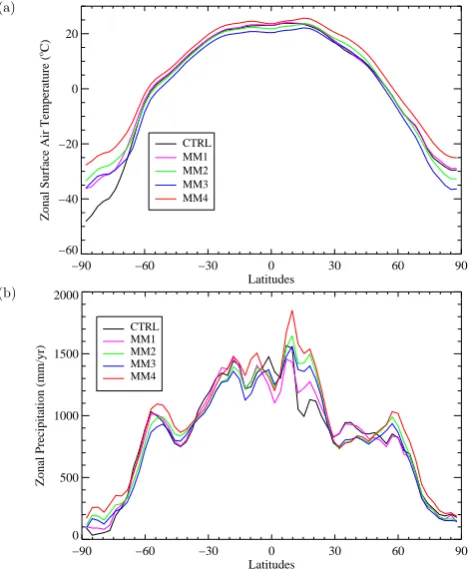
Fig. 4. Zonal average (a) surface air temperature (◦C) and (b)

pre-cipitation (mm/yr) for the series of simulation experiments MM1 to MM4.

2.1.6 Orbital configuration

As we refer for the MMCO to a time span of about two mil-lion years integrated over several orbital cycles, we applied a present-day orbital configuration (eccentricity 0.016724◦, obliquity 23.446◦and longitude of perihelion 102.04◦) and solar constant (1365 W/m2) for the whole series of experi-ments. To test the potential effect of such a warm orbital configuration on the MMCO climate we performed an addi-tional experiment where we applied a cold LGM orbital con-figuration (eccentricity 0.018994◦, obliquity 22.949◦, longi-tude of perihelion 114.42◦ and present-day solar constant) under MMCO boundary conditions similar to those in ex-periment MM4. The “cold” orbital configuration induced a global temperature decrease of−0.1◦_{C in comparison to}

(7)

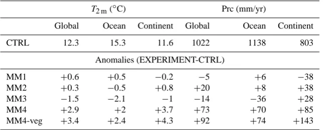
Table 2. Global, continental and oceanic annual mean near-surface temperatureT2m (◦C) and precipitation (mm/yr) anomalies for the

five Middle Miocene simulation experiments. The continental mean excludes the contribution from Antarctica since strong warming can be attributed due to the absence of ice that is not representative of the other effects on the continents. All results reported here are global means over the last 20 years of 50-year simulations, allowing 30 years for the model to equilibrate. The CTRL absolute values are shown for reference.

T2 m(◦C) Prc (mm/yr)

Global Ocean Continent Global Ocean Continent

CTRL 12.3 15.3 11.6 1022 1138 803 Anomalies (EXPERIMENT-CTRL)

MM1 +0.6 +0.5 −0.2 −5 +6 −38 MM2 +0.3 −0.5 +0.8 +20 +8 +38 MM3 −1.5 −2.1 −1 −14 −36 +28 MM4 +2.9 +2 +3.7 +73 +70 +85 MM4-veg +3.4 +2.4 +4.3 +92 +74 +143

3 Results

3.1 Experiment MM1: surface ocean and ice-sheet boundary conditions

Experiment MM1 shows a global temperature increase of +0.6◦C (see Table 2) that is mainly due to oceanic warm-ing and Antarctic and Greenland warmwarm-ing in the absence of land-ice, whereas the temperatures and precipitation on other continents decrease. The zonal averages of surface air temperature (SAT) and precipitation are shown in Fig. 4. The zonal average temperature and precipitation anomalies (MM1–CTRL) are also shown in Fig. 5 to allow a finer com-parison. The MM1 zonal temperature averages do not in-dicate large differences from the control experiment at any latitude, except at high latitudes of both hemispheres. The warming at high latitudes linked to an increase of precipita-tion is due to the absence of ice on land.

Figure 6 shows the annual mean surface air tempera-ture (SAT) and precipitation anomalies between experiment MM1 and the control run CTRL. Large increases of the sur-face air temperature occur over Greenland and especially Antarctica. The absence of ice on Antarctica and Green-land strongly decreases the surface albedo that induces large warming and a decrease of the snow cover, leading to a pos-itive albedo feedback during summer in each Hemisphere (not shown). However, in winter the influence of surround-ing colder oceanic air masses induces a net coolsurround-ing of about −1◦C over Greenland. Large precipitation disruptions oc-cur in the tropics and sub-tropics as well as over the North Atlantic Ocean.

Significant changes in surface air temperature as well as in precipitation are obtained especially over the oceans. These are a consequence of the sea surface temperature modifica-tion in response to ocean circulamodifica-tion changes in the Miocene LSG simulation. The reduction of the heat transfer to the

North Atlantic leads to large decreases of SAT in that re-gion. Colder and drier conditions are obtained along the south-west coast of North America but the strongest decrease of SAT, of up to−6◦_{C, occurs in the North Atlantic, along}

the south coast of Greenland. This region also experiences a large decrease of precipitation linked to the cooling of the air masses. The colder conditions over the North Atlantic induce continental temperature decreases together with pre-cipitation increase, notably over northwestern Europe and Africa in winter. However, the decrease of precipitation of about−400 mm/yr over the northern part of South America and the east coast of North America, linked to a decrease of surface evaporation, leads to a surface temperature increase of more than 1◦C.

The opening of the Central American Seaway and the clo-sure of the Bering Strait, which inhibits the influx of fresh and cold water from the Arctic Ocean into the Pacific in-duces warming in the North Pacific, reaching+4◦C along the west coast of North America together with a precipi-tation increase. This brings warmer and more humid air masses from the West to the Centre of North America and warmer air masses to the East after the passage of the high North American reliefs.

(8)

(a)

−90 −60 −30 0 30 60 90

Latitudes −10

−5 0 5 10 15 20 25

Zonal Surface Air Temperature Anomaly (

oC) MM1

MM2 MM3 MM4

(b)

−90 −60 −30 0 30 60 90

Latitudes −200

0 200 400

Zonal Precipitation Anomaly (mm/yr)

MM1 MM2 MM3 MM4 (a)

−90 −60 −30 0 30 60 90

Latitudes −10

−5 0 5 10 15 20 25

Zonal Surface Air Temperature Anomaly (

oC) MM1

MM2 MM3 MM4

(b)

−90 −60 −30 0 30 60 90

Latitudes −200

0 200 400

Zonal Precipitation Anomaly (mm/yr)

MM1 MM2 MM3 MM4

Fig. 5. Zonal average (a) surface air temperature anomalies (◦C)

and (b) precipitation anomalies (mm/yr) for the series of Middle Miocene simulation experiments MM1 to MM4.

prevails in the presence of an open Tethys Seaway. However, since precipitation is strongly decreased in India during sum-mer, the warming in this region can be linked to a reduced monsoon activity in presence of an open Eastern Tethys Sea-way. Strong decreases of precipitation also occur in Indone-sia and South-East China, suggesting a reduced monsoon ac-tivity in these regions too. Finally, the SAT cools by about −2◦C in eastern Russia, extending the cooling trend over Europe to the east.

3.2 Experiment MM2: topography

The reduction of the topography in experiment MM2 gen-erates the weakest effect in magnitude on global tempera-ture in our series of experiments. It causes a global mean cooling of−0.3◦_{C relative to experiment MM1, if we}

as-sume that the topographic and oceanic boundary conditions effects are independant of each other. However, the reduc-tion of the topography significantly increases precipitareduc-tion, especially on the continents (see Table 2). The lowering of the topography leads to a global decrease of temperature over the oceans whereas it leads to an increase of temperature over the continents. These opposite temperature effects over the oceans and continents can be explained by the conservation of the mass of the atmosphere in our model. The lowering of

(a) Surface Air Temperature Anomaly (MM1)

180o 120oW 60oW 0o 60oE 120oE 180o 90oS

−10.0 −8.0 −6.0 −4.0 −2.0 −1.0 −0.5 −0.2 0.0 0.2 0.5 1.0 2.0 4.0 6.0 8.0 10.0 Surface Temperature (o

C)

(b) Precipitation Anomaly (MM1)

180o 120oW 60oW 0o 60oE 120oE 180o 90oS

−400 −350 −300 −250 −200 −150 −100 −50 0 50 100 150 200 250 300 350 400 Precipitation (mm/yr)

(a) Surface Air Temperature Anomaly (MM1)

180o 120oW 60oW 0o 60oE 120oE 180o 90oS

C)

(b) Precipitation Anomaly (MM1)

180o 120oW 60oW 0o 60oE 120oE 180o 90oS

Fig. 6. (a) Annual mean surface temperature and (b) precipitation

anomalies (MM1-minus-CTRL) for experiment MM1. Only the precipitation anomalies greater than one standard deviation for the long-term annual mean over the last 20 simulation years are shown.

the topography induces a surface pressure increase on land that leads to a surface pressure decrease over the oceans that in turn cools the oceans. Nevertheless, local surface sure changes occur due to the displacement of high/low pres-sure cells in response to topography reduction. The lowering of the topography also produces localized warming, notably over Antarctica and around 30◦N over the lowered reliefs. However, it decreases the temperatures at latitudes higher than 60◦N (see Fig. 4). The lowering also decreases pre-cipitation around 30◦N but strongly increases precipitation especially in the tropics around the ITCZ (see Fig. 5).

(9)

(a) Surface Air Temperature Anomaly (MM2 − MM1)

180o 120oW 60oW 0o 60oE 120oE 180o 90oS

C)

(b) Precipitation Anomaly (MM2 − MM1)

180o 120oW 60oW 0o 60oE 120oE 180o 90oS

−10.0 −8.0 −6.0 −4.0 −2.0 −1.0 −0.5 −0.2 0.0 0.2 0.5 1.0 2.0 4.0 6.0 8.0 10.0 Surface Temperature (o_C)

180o 120oW 60oW 0o 60oE 120oE 180o 90oS

anomalies between experiments MM2 and MM1. Only the precip-itation anomalies greater than one standard deviation for the long-term annual mean over the last 20 simulation years are shown.

also strongly disturbs the annual precipitation anomaly dis-tribution on the continents (see Fig. 7). The anomalies show large differences when compared to the anomalies in experi-ment MM1. Northern and western Europe experience a SAT decrease that extends to the east. The annual anomaly es-sentially reflects the colder conditions that affect Eurasia in summer, whereas warmer conditions prevail in winter (see Fig. 8). Precipitation also strongly increases over northern Europe especially in summer (see Fig. 9). As illustrated in Figs. 10 and 11, showing respectively the summer and winter low-level winds (850 hPa) for experiments CTRL and MM2, seasonal effects can be due to a more zonal atmospheric sur-face circulation in the presence of lower reliefs. Therefore stronger and more direct winds from the North Atlantic flow across Europe and penetrate deeper into the continent, bring-ing more humid and colder conditions in summer and more humid and warmer conditions in winter, weakening the sea-sonal contrast of temperature and precipitation over Europe. This strong effect of the lower reliefs on the precipitation

(a) JJA Surface Air Temperature Anomaly (MM2 − MM1)

180o 120oW 60oW 0o 60oE 120oE 180o 90oS

C)

(b) DJF Surface Air Temperature Anomaly (MM2 − MM1)

180o 120oW 60oW 0o 60oE 120oE 180o 90oS

C)

(a) JJA Surface Air Temperature Anomaly (MM2 − MM1)

180o 120oW 60oW 0o 60oE 120oE 180o 90oS

C)

(b) DJF Surface Air Temperature Anomaly (MM2 − MM1)

180o 120oW 60oW 0o 60oE 120oE 180o 90oS

C)

Fig. 8. Surface air temperature anomalies in (a) Northern

Hemi-sphere summer (JJA) and (b) Northern HemiHemi-sphere winter (DJF) between experiments MM2 and MM1.

distribution in northern Europe is discussed in more detail in Sect. 3.2.1. Westerly winds coming from the North Amer-ican continent instead of the Labrador Sea also flow over the North Atlantic, decreasing the activity of the Iceland low pressure cell. However, the southern part of Europe expe-riences an increase of SAT that is linked to the reduction of topography in the Alps and other reliefs, inducing local warming that dominates over the other effects. Furthermore, this warming can be reinforced in winter by a decrease of snowfall, resulting from the positive snow albedo feedback.

North America is affected by warming of more than+2◦_C

(10)

(a) JJA Precipitation Anomaly (MM2 − MM1)

180o 120oW 60oW 0o 60oE 120oE 180o 90oS

(b) DJF Precipitation Anomaly (MM2 − MM1)

180o 120oW 60oW 0o 60oE 120oE 180o 90oS

(a) JJA Precipitation Anomaly (MM2 − MM1)

180o 120oW 60oW 0o 60oE 120oE 180o 90oS

(b) DJF Precipitation Anomaly (MM2 − MM1)

180o 120oW 60oW 0o 60oE 120oE 180o 90oS

Fig. 9. Precipitation anomalies in (a) Northern Hemisphere

sum-mer (JJA) and (b) Northern Hemisphere winter (DJF) between ex-periments MM2 and MM1.

Centre of North America, the lower Rockies also weaken the frontal zone activity in summer between air masses coming from the West and the East. This leads to a decrease of sur-face evaporation that decreases precipitation in summer and contributes to warm the region.

The decrease of the height of the Tibetan Plateau also pro-duces large seasonal impacts. SAT increases for the whole year over China and eastern Russia, but decreases over In-dia, Indonesia and Australia. As expected, a lower Tibetan Plateau contributes to weaken the Asian monsoon activity, which is characterized by a decrease of precipitation in sum-mer. The summer precipitation also decreases in Indonesia and the eastern Equatorial Pacific, where the surface winds weaken. North-East China gets drier during the whole year, due to a strengthening of the continental winds coming from the North-East in winter, but a decrease of the South-East winds in summer, which bring less humidity.

Africa is affected by an increase of SAT that can be di-rectly attributed to the topographic reduction in the North and the South-East. However, SAT decreases in West and

(a) JJA Low Level Winds (CTRL)

180o 120oW 60oW 0o 60oE 120oE 180o 90oS

20 m/s

(b) DJF Low Level Winds (CTRL)

180o 120oW 60oW 0o 60oE 120oE 180o 90oS

20 m/s (a) JJA Low Level Winds (CTRL)

180o 120oW 60oW 0o 60oE 120oE 180o 90oS

20 m/s

(b) DJF Low Level Winds (CTRL)

180o 120oW 60oW 0o 60oE 120oE 180o 90oS

20 m/s

Fig. 10. Low-level winds (850 hPa) for the CTRL experiment in (a)

Northern Hemisphere summer and (b) Northern Hemisphere winter.

Central Africa. This last effect comes together with a strong increase of precipitation, that can be attributed to the deeper penetration of westerly winds from the Atlantic together with a deeper penetration of north-easterly winds, which come from the moist region of the open Eastern Tethys Seaway. The northern part of South America also experiences a de-crease of SAT together with a strong inde-crease of precipita-tion.

3.2.1 Effects of the topography on precipitation in Europe

(11)

(a) JJA Low Level Winds (MM2)

180o 120oW 60oW 0o 60oE 120oE 180o 90oS

20 m/s

(b) DJF Low Level Winds (MM2)

180o 120oW 60oW 0o 60oE 120oE 180o 90oS

20 m/s (a) JJA Low Level Winds (MM2)

180o 120oW 60oW 0o 60oE 120oE 180o 90oS

20 m/s

(b) DJF Low Level Winds (MM2)

180o 120oW 60oW 0o 60oE 120oE 180o 90oS

20 m/s

Fig. 11. Low-level winds (850 hPa) for the MM2 experiment in (a)

Northern Hemisphere summer and (b) Northern Hemisphere winter.

MM2-A) and both together (experiment MM2-AE). We only lower the North American and European reliefs for this se-ries of tests. The other reliefs are hold at their respective present-day elevations.

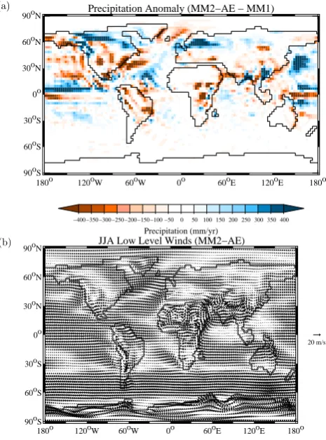
The disruption of summer precipitation and the summer winds at 850 hPa in the absence of European reliefs are shown in Fig. 12. The lower reliefs in North Europe allow stronger westerly winds that come more directly from the Atlantic Ocean to penetrate deeper into the continent, bring-ing more humid and cold oceanic air masses to northern Eu-rope. Nevertheless, the lowering of the North European re-liefs alone is not sufficient to form the wet tongue that we obtained in experiment MM2.

The lowering of the North American reliefs also produces stronger and more direct summer westerly winds in north-western Europe, generating more precipitation in the region (see Fig. 13). However the presence of the North European reliefs stops the wetter air masses coming from the West, and does not allow the wet tongue obtained in experiment MM2 to form neither. Precipitation increases in northwest-ern Europe similar in terms of magnitude to those found in experiment MM2 are only obtained when the effects of Eu-ropean and North American topography changes are com-bined (Fig. 14). We also perform additional sensitivity ex-periments testing separately the effects of the lowering of the

(a) Precipitation Anomaly (MM2−E − MM1)

180o 120oW 60oW 0o 60oE 120oE 180o 90oS

(b) JJA Low Level Winds (MM2−E)

180o 120oW 60oW 0o 60oE 120oE 180o 90oS

20 m/s (a) Precipitation Anomaly (MM2−E − MM1)

180o 120oW 60oW 0o 60oE 120oE 180o 90oS

(b) JJA Low Level Winds (MM2−E)

180o 120oW 60oW 0o 60oE 120oE 180o 90oS

20 m/s

Fig. 12. (a) Annual mean precipitation anomalies (MM2-E–MM1)

and (b) Northern Hemisphere summer low-level winds (850 hPa) for experiment MM2-E that considers a reduced topography only in Europe.

Tibetan Plateau, African reliefs and South American reliefs on the precipitation distribution in Europe. Effects on Eu-ropean precipitation and teleconnections found in these later experiments are rather weak (not shown). We conclude that the reduction of topography in North America and Europe is necessary to produce the colder and wetter conditions that prevail in North Europe in experiment MM2. However, the wet tongue does not extend to the East as far as it does in experiment MM2. We can therefore attribute the increase of precipitation in North West Asia to the reduction of the to-pography in Asia.

3.3 Experiment MM3: low CO2

(12)

(a) Precipitation Anomaly (MM2−A − MM1)

180o 120oW 60oW 0o 60oE 120oE 180o 90oS

(b) JJA Low Level Winds (MM2−A)

180o 120oW 60oW 0o 60oE 120oE 180o 90oS

20 m/s (a) Precipitation Anomaly (MM2−A − MM1)

180o 120oW 60oW 0o 60oE 120oE 180o 90oS

(b) JJA Low Level Winds (MM2−A)

180o 120oW 60oW 0o 60oE 120oE 180o 90oS

20 m/s

Fig. 13. Same as Fig. 12 for experiment MM2-A that considers

a reduced topography only in North America.

experiments MM3 and MM2 are shown in Fig. 15. The 80 ppmv lowering of the CO2concentration induces a rather uniform temperature cooling of about−2◦C. The magnitude of the cooling is similar over continents and oceans, and in both Northern and Southern Hemispheres. Stronger cool-ing occurs at high latitudes, especially over the Arctic and Antarctic Oceans, due to sea-ice feedback. The decrease of the CO2concentration does not disrupt the precipitation dis-tribution when compared to experiment MM2. It slightly de-creases the precipitation over the tropical oceans.

3.4 Experiment MM4: high CO2

The increase of the atmospheric CO2 concentration to 500 ppmv in experiment MM4 has the strongest effect on temperature of the series. It warms the global climate by +2.6◦_{C. The higher CO}

2level also reinforces the increase of precipitation caused by the reduction of the topography, producing the strongest effects of the four experiments on precipitation. The increase of atmospheric CO2 reinforces the warming at high latitudes, reducing again the latitudinal temperature gradient (see Fig. 4). This high-latitude warm-ing can be attributed to the meltwarm-ing of sea-ice under warmer conditions. The CO2 induced warming also contributes to

(a) Precipitation Anomaly (MM2−AE − MM1)

180o 120oW 60oW 0o 60oE 120oE 180o 90oS

(b) JJA Low Level Winds (MM2−AE)

180o 120oW 60oW 0o 60oE 120oE 180o 90oS

20 m/s (a) Precipitation Anomaly (MM2−AE − MM1)

180o 120oW 60oW 0o 60oE 120oE 180o 90oS

(b) JJA Low Level Winds (MM2−AE)

180o 120oW 60oW 0o 60oE 120oE 180o 90oS

20 m/s

Fig. 14. Same as Fig. 12 for experiment MM2-AE that considers

a reduced topography only in North America and in Europe.

increase the precipitation rate at all latitudes. The differ-ence in surface air temperature between experiments MM4 and MM3, equal to +4.4◦C, corresponds to the climate sen-sitivity of the model to a CO2increase of 300 ppmv under Middle Miocene conditions. Thus, the Miocene sensitivity to a doubling of CO2must be of the order of 3.3◦C (using the temperature increase between experiment MM4 and MM3 as a reference), if we assume that the global mean tempera-ture variation is proportional to the radiative forcing (Forster et al., 2007), and radiative forcing is proportional to the log-arithm ofpCO2ratios (Myhre et al., 1998). In comparison, we obtained a climate sensitivity to a doubling of CO2from a preindustrial level of 280 ppmv to 560 ppmv of +4.5◦_{C under}

a present-day configuration. The model climate sensitivity is thus significantly smaller under Middle Miocene conditions. That could be partially explained by the reduction of the sea-ice extent at Middle Miocene, which is very sensitive to CO2 changes in our model.

(13)

180o 120oW 60oW 0o 60oE 120oE 180o 90oS

C)

180o 120oW 60oW 0o 60oE 120oE 180o 90oS

anomalies between experiments MM3 and MM2.

in some regions. Northwestern Europe notably experiences significant increases of temperature in experiment MM4, whereas the reduced topography alone induced a cooling in that region (see Sect. 3.2.1). The higher CO2concentration also produces a stronger warming at high latitudes and espe-cially over the Arctic and Southern Oceans due to the melting of sea-ice. However, the higher CO2concentration does not disturb the precipitation distribution induced by the reduction of the topography in experiment MM2. The distributions of the precipitation anomalies are quite similar in experiments MM2 and MM4. The CO2effect reinforces the precipitation increases especially in the tropics.

3.5 Experiment MM4-veg: vegetation

The warmer and more humid conditions prevailing in experi-ment MM4 could lead to significant vegetation cover modifi-cations that could in turn affect the climate. Here, we analyse the results of experiment MM4-veg, taking into account the vegetation changes in response to the MM4 climate, in order to quantify the order of magnitude and the local impacts of vegetation changes on the MMCO climate.

180o 120oW 60oW 0o 60oE 120oE 180o 90oS

anomalies between experiments MM4 and MM2.

(14)

32 A.-J. Henrot et al.: Middle Miocene climate modelling experiments

Fig. 17. Biome distributions from CARAIB preindustrial and MMCO equilibrium runs.

Fig. 17. Biome distributions from CARAIB preindustrial and MMCO equilibrium runs.

at the east coast of North America and in Southeastern China lead to the replacement of subtropical forests by warm and open woodlands.

The anomalies between experiments MM4-veg and MM4 are shown in Fig. 18 in order to isolate the vegetation effects from the other forcings applied in experiment MM4. Glob-ally, experiment MM4-veg shows the strongest global tem-perature and precipitation increases of the series of Miocene experiments (see Table 2), especially on the continents due to the vegetation change impact. In comparison with exper-iment MM4 the vegetation changes produce an additional global warming of +0.5◦C (+0.4◦C over the oceans and +0.6◦C over the continents) and an increase of precipitation of +19 mm/yr (+4 mm/yr over the oceans and+58 mm/yr over the continents). Locally, the vegetation contribution is only slightly lower in terms of magnitude than the contri-butions of topography and high atmospheric CO2level. As described in Sect. 2, vegetation cover changes affect surface albedo and roughness length, but the albedo impact on sur-face temperature is dominant, because of its direct impact on the energy balance (Henrot, 2007). The changes in rooting depth mainly affect the water cycle and therefore precipita-tion. The differences between the surface albedo and rooting

depth derived from the Miocene and the preindustrial vege-tation distributions are shown in Fig. 19.

(15)

(a) Surface Air Temperature Anomaly (MM4−veg − MM4)

180o 120oW 60oW 0o 60oE 120oE 180o 90oS

C)

(b) Precipitation Anomaly (MM4−veg − MM4)

180o 120oW 60oW 0o 60oE 120oE 180o 90oS

(a) Surface Air Temperature Anomaly (MM4−veg − MM4)

180o 120oW 60oW 0o 60oE 120oE 180o 90oS

(b) Precipitation Anomaly (MM4−veg − MM4)

180o 120oW 60oW 0o 60oE 120oE 180o 90oS

anomalies between experiment MM4-veg and MM4.

leading to an increase of evaporation and precipitation. The same effect occurs in central Asia. The precipitation increase in Equatorial Africa is due to the expansion of the tropical forests which enhances the hydrological cycle. The precipi-tation decrease along the west coast of Europe is due to the replacement of temperate forests by open woodlands, which decreases the soil water content.

4 Discussion

In our series, experiment MM1 assesses the climatic effects of the MMCO surface ocean heat flux distribution, derived from Miocene LSG model simulation (Butzin et al., 2010). These changes produce contrasted effects on surface air tem-perature and precipitation over the oceans that influence the climatic conditions on land. The reduction of the oceanic heat transfer to the North Atlantic due to the opening of the Central American Seaway brings colder conditions over the North Atlantic and northwestern Europe. This effect agrees with the majority of published modelling studies results indi-cating that the closure of the Central American Seaway was

(a)

180o 120oW 60oW 0o 60oE 120oE 180o 90oS

−25.0−20.0−15.0−10.0 −5.0 −2.0 −1.0 −0.5 0.0 0.5 1.0 2.0 5.0 10.0 15.0 20.0 25.0 Surface Albedo

(b)

180o 120oW 60oW 0o 60oE 120oE 180o 90oS

−25.0−20.0−15.0−10.0 −5.0 −2.0 −1.0 −0.5 0.0 0.5 1.0 2.0 5.0 10.0 15.0 20.0 25.0 Rooting Depth (cm)

(a)

180o 120oW 60oW 0o 60oE 120oE 180o 90oS

−25.0−20.0−15.0−10.0 −5.0 −2.0 −1.0 −0.5 0.0 0.5 1.0 2.0 5.0 10.0 15.0 20.0 25.0 Surface Albedo

(b)

180o 120oW 60oW 0o 60oE 120oE 180o 90oS

−25.0−20.0−15.0−10.0 −5.0 −2.0 −1.0 −0.5 0.0 0.5 1.0 2.0 5.0 10.0 15.0 20.0 25.0 Rooting Depth (cm)

Fig. 19. (a) Surface albedo difference and (b) rooting depth

differ-ence between experiment MM4-veg and CTRL.

responsible for increased oceanic heat transport to the North Atlantic that brought warmer conditions and ultimately in-creased precipitation in the Northern Hemisphere (Lunt et al., 2008; Schneider and Schmittner, 2006). The decrease of pre-cipitation in South Asia, linked to SST changes, indicates a weakening of the Asian monsoon. According to Tschuck et al. (2004), the weakening of the Asian monsoon can be linked to the increase of sea surface temperatures in the equa-torial Indian Ocean and western Pacific Ocean. Therefore, the warmer conditions induced in the Pacific by the opening of the Central American Seaway may be contributing to the reduction of the precipitation in some parts of Asia.

(16)

690 A.-J. Henrot et al.: Middle Miocene climate modelling experiments the Tibetan Plateau and European reliefs. Moreover, the

re-duced height of the Tibetan Plateau prevents the development of a monsoon-like circulation (Kutzbach et al., 1989; Harris, 2006) that induces a strong decrease of precipitation in East Asia. Recently, Herold et al. (2009) focused on the effect of lowered Tibetan Plateau and Andes on the Middle Miocene climate using the NCAR model (CAM v.3.1) and Commu-nity Land Model (CLM v.3.0) coupled to a slab ocean model with fixed sea-surface temperatures. Herold et al. (2009) also obtained strong local warming and a significant disrup-tion of the surface winds due to the reducdisrup-tion of elevadisrup-tion over the Tibetan Plateau. However, the prescription of fixed sea-surface temperature in their experiment precluded a re-sponse of the ocean and therefore of the Asian monsoon sys-tem. Nevertheless, they also pointed out that the lowering of the Tibetan Plateau leads to a cooling linked to snow depth increase in Central Eurasia. In our experiment MM2, the reduction of the topography leads to slight warming in Eura-sia, and does not significantly alter the snow depth in the region. Therefore, we can attribute the Eurasian warming in our results to the local increase of temperature induced by the reduction of reliefs higher than 400 m in the region. Unfortunately, our setup does not allow us to isolate the in-fluence on Eurasia of the Tibetan Plateau elevation change. The lowering of North American and European reliefs pro-duces wetter and colder conditions over northwestern Eu-rope that are in disagreement with proxy-based reconstruc-tions of the European Middle Miocene climate (Mosbrugger et al., 2005). However, the reduction of the seasonal gra-dient and the warming in South and Central Europe agree well with several reconstructions of the Middle Miocene cli-mate based on pollen analysis (Jimenez-Moreno and Suc, 2007) and mega- or microfloral records (Mosbrugger et al., 2005; Utescher et al., 2007). Moreover, the reconstruction of Utescher et al. (2007) and other reconstructions based on the analysis of small mammals (Van Dam, 2006) showed ev-idence for the persistence of a European wet zone during the Miocene, in agreement with our results. Nevertheless, the maximum increases of precipitation are located further north in Europe where no proxy reconstruction is available.

In the next two experiments (MM3 and MM4) we test the effect of various CO2concentrations on the middle Miocene climate. The CO2 effect is rather uniform on the conti-nents and the oceans of both hemispheres. However, the combination of the CO2 and topographic effects in exper-iment MM4 generates a stronger warming over the conti-nents than over the oceans, which is also seen in the re-sults of Tong et al. (2009). The rere-sults of experiment MM4 over northwestern Europe show a slight increase of tempera-ture, since the topography induced effect cooled that region. Both the topography reduction and increased CO2 concentra-tion contribute to wetter and warmer condiconcentra-tions in Europe, in better agreement with the proxies reconstructions (Mos-brugger et al., 2005; Utescher et al., 2007). As in Tong et al. (2009), the increase of the CO2 concentration warms

the high latitudes reducing the latitudinal gradient and also increases the precipitation. The increase of the CO2 concen-tration furthermore enhances the hydrological cycle in the tropics, according to Tong et al. (2009). Nevertheless the ac-tivity of the monsoon system is still reduced in experiment MM4. This confirms the dominant effect of topography on the Asian monsoon system as compared to the CO2 contri-bution (Tong et al., 2009).

Experiment MM4-veg finally allows us to investigate the vegetation feedback on climate in response to a warm and humid climate for the MMCO. The simulated vegetation dis-tribution forced with the climate of experiment MM4 mainly demonstrates a reduction of the desert and sub-desert areas in the benefit of grasslands and forests, as well as an ex-pansion of warm forest types poleward of the subtropical zone. This fairly agrees with the Middle Miocene data-based vegetation reconstruction used as boundary condi-tion in the study of Tong et al. (2009), despite the differ-ences in plant type classifications. Our vegetation distribu-tion also agrees over South and Central Europe with the re-construction of Utescher et al. (2007), which suggested the presence of warm mixed and broadleaved evergreen forests in South and Central Europe. Consistently with the data from Jimenez-Moreno and Suc (2007), CARAIB also yields warm and open mixed forest in Southwest Europe, whereas it leads to thermophilous and mesothermic elements in Central Europe. Such a change in the vegetation cover contributes to maintain and even to increase the warm and humid condi-tions that prevailed in experiment MM4.

In the series of sensitivity tests, several experiments re-sult in an increase of the global surface air temperature. The increase of the atmospheric CO2concentration to 500 ppmv in experiment MM4 produces the strongest global warming of the series of four experiments, as compared to the warm-ing produced by oceanic heat transport and ocean gateway changes (experiment MM1) or reduced topography (experi-ment MM2). A lower than preindustrial CO2concentration cools the global climate. A higher CO2concentration seems therefore necessary to generate a warmer climate in the Mid-dle Miocene. The lower climate sensitivity of the climate model under Middle Miocene conditions may partly explain the requirement of the model for high CO2to produce sig-nificant temperature increases at the MMCO. However the warming we obtain is much lower than suggested by proxy data (Mosbrugger et al., 2005; Zachos et al., 2001), which witness temperatures at middle latitudes up to 6◦_{C higher}

(17)

A.-J. Henrot et al.: Middle Miocene climate modelling experiments 691 an atmospheric CO2concentration of 700 ppmv in

compari-son to a present-day control run with a reference CO2 con-centration equal to 379 ppmv. You et al. (2009) used the same models to test the effect of various CO2 concentra-tions together with several sea surface temperature gradients. They obtained temperature increases of+2.3◦C for an at-mospheric CO2concentration of 350 ppmv and a high SST gradient and of+3.5◦C for CO2at 700 ppmv and a medium SST gradient. Micheels et al. (2009a) used the Planet Sim-ulator to test the sensitivity of the Late Miocene climate (Tortonian) to various CO2 concentrations. They obtained global warming between+2.3◦C for 280 ppmv and+3.7◦C for 460 ppmv in comparison to a preindustrial control run with a CO2 concentration of 280 ppmv. In comparison to our results, Micheels et al. (2009a) found a greater warm-ing under lower CO2concentration with the Planet Simula-tor. This effect could be due to the differences in the bound-ary conditions they used for the Late Miocene. They no-tably adopted a present-day ocean heat flux distribution, in-cluding a stronger Gulf Stream than used here and a lower topography on land in some regions. They also prescribed a vegetation distribution for the Late Miocene, where all the desert areas were replaced by forest or grassland ecosystems and the boreal forests shifted further North, whereas we did not consider any vegetation change in the MM1 to MM4 simulation experiments.

The model results consistently indicate that a higher than present-day CO2 concentration is necessary to pro-duce a warm Middle Miocene climate (You et al., 2009; Tong et al., 2009). In that sense, the model results support the terrestrial proxy reconstruction suggesting higher atmo-spheric CO2concentrations at the MMCO, between 300 and 850 ppmv (K¨urschner et al., 2008; Retallack, 2009). Con-versely modelling results do not support the low CO2 con-centration, between 140 and 300 ppmv, derived from ma-rine isotopic records, that suggest a decoupling between CO2 and temperature during the Middle Miocene (Henderiks and Pagani, 2008; Pearson and Palmer, 2000). Experiments us-ing lower CO2concentrations generate colder climate than at present-day (experiment MM3 in this study, Tong et al., 2009 or You et al., 2009). However, as recently discussed by Pa-gani et al. (2010, Supplement) CO2concentrations during the Miocene could possibly have been higher than suggested by previous estimates based on planktonic foraminiferalδ18O temperature reconstructions. Correcting for inherent biases could thus help to reconcile model results to proxy-based reconstructions. However, as emphasised by Diester-Haass et al. (2009), a high CO2level at the Middle Miocene would be difficult to reconcile with the highδ13C values of benthic foraminifera, which suggest large deposition rates of organic carbon tending to reduce atmospheric CO2levels. Therefore model results should be interpreted with care.

We indeed do not take into account all the possible effects that could contribute to the Middle Miocene warm climate. We notably miss the feedback of climate on ocean

circu-lation at Middle Miocene, which could only be simulated with a fully coupled ocean-atmosphere model, since we used a slab ocean model as in previous studies (Tong et al., 2009; You et al., 2009). The opening of ocean gateways notably at low latitudes seems to have strongly contributed to modify the global ocean circulation in the Cenozoic in comparison to present-day (Bice et al., 2000; Von der Heydt and Dijkstra, 2008). We also only tested the effect of various CO2 concen-trations on climate given the large uncertainty in CO2 esti-mations. We did not take into account a change in the con-centrations of other atmospheric greenhouse gases such as methane. The potential role of such feedbacks is well illus-trated by the results of our simulation experiment MM4-veg, which takes into account the feedback on climate from the changing vegetation cover compared to the first four simula-tion experiments of our series.

5 Conclusions

In this study, we examine the potential contributions of sev-eral boundary condition changes to the warm climate of the Middle Miocene and particularly the Middle Miocene Climatic Optimum (MMCO). We used the Planet Simula-tor, an Earth System model of intermediate complexity to investigate the contributions of the absence of ice on the continents, the opening of the Central American and East-ern Tethys Seaways, the lowering of the topography on land and the effect of various atmospheric CO2 concen-trations on the Middle Miocene climate. We also investi-gated the feedback of vegetation on climate. Therefore, we prescribe vegetation cover changes derived from a MMCO vegetation distribution produced by the dynamic vegetation model CARAIB, forced with the climate of the warmest and most humid experiment of the series. The boundary condition changes generally produce global warming in the Middle Miocene that are in agreement with previous Mid-dle Miocene sensitivity experiments (Tong et al., 2009; You et al., 2009). However, the increases of temperature that we obtained are lower than those supported by proxy data (Zachos et al., 2001; Bruch et al., 2007).