www.atmos-meas-tech.net/10/199/2017/ doi:10.5194/amt-10-199-2017
© Author(s) 2017. CC Attribution 3.0 License.
Cloud detection in all-sky images via multi-scale neighborhood
features and multiple supervised learning techniques
Hsu-Yung Cheng1and Chih-Lung Lin2
1Department of Computer Science and Information Engineering, National Central University, No. 300 Jhongda Rd., Jhongli City, Taoyuan 32001, Taiwan
2Department of Electronic Engineering, Hwa Hsia University of Technology, New Taipei City, Taiwan
Correspondence to:Hsu-Yung Cheng ([email protected])
Received: 18 May 2016 – Published in Atmos. Meas. Tech. Discuss.: 9 August 2016 Revised: 23 December 2016 – Accepted: 23 December 2016 – Published: 17 January 2017
Abstract. Cloud detection is important for providing nec-essary information such as cloud cover in many applica-tions. Existing cloud detection methods include red-to-blue ratio thresholding and other classification-based techniques. In this paper, we propose to perform cloud detection us-ing supervised learnus-ing techniques with multi-resolution fea-tures. One of the major contributions of this work is that the features are extracted from local image patches with different sizes to include local structure and multi-resolution informa-tion. The cloud models are learned through the training pro-cess. We consider classifiers including random forest, sup-port vector machine, and Bayesian classifier. To take advan-tage of the clues provided by multiple classifiers and various levels of patch sizes, we employ a voting scheme to com-bine the results to further increase the detection accuracy. In the experiments, we have shown that the proposed method can distinguish cloud and non-cloud pixels more accurately compared with existing works.
1 Introduction
With the trend of sustainable and green energy, there is a growing demand for solar energy technology. To utilize so-lar energy effectively, integrated and so-large-scale photovoltaic systems need to overcome the unstable nature of solar re-source (Gueymard, 2004; Heinemann et al., 2006; Lorenz et al., 2009). The ability to forecast surface solar irradiance is helpful for planning and deployment of electricity generated by different units. Numerical weather prediction information or satellite images are popular materials used for wide-range
prediction (Marquez and Coimbra, 2011; Perez et al., 2002, 2010; Remund et al., 2008). However, the resolution of pre-diction with respect to space and time obtained by weather prediction information or satellite cloud images is relatively coarse compared to the resolution desired for photovoltaic grid operators. For more refined spatial and temporal resolu-tion of irradiance predicresolu-tion, research that analyzes images obtained from devices capturing skies has emerged. Ground-based sky camera systems have been proposed to capture the images of the sky (Sabburg and Wong, 1999), allowing researchers to study the relationship between the sun and clouds and the effect of clouds. Devices developed to moni-tor the sky presented in some of the pioneering works include whole sky imager (Kassianov et al., 2005; Li et al., 2004), whole sky camera (Long et al., 2006), all-sky imager (Kub-ota et al., 2003), and t(Kub-otal sky imager (Pfister et al., 2003). More recent commercial products include all-sky cameras by Eko Instruments, Oculus, and SBIG. These devices are use-ful to make up the deficiency of satellite cloud observations in terms of spatial and temporal resolutions.
nega-tively correlated under most conditions. In addition to pro-viding cloud coverage information, accurate cloud detection result could further improve the cloud type classification ac-curacy (Cheng and Yu, 2015b). It has been established that employing cloud type information in the process of short-term irradiance prediction could yield more accurate predic-tion results (Cheng and Yu, 2015a).
Cloud detection in all-sky image decides if a pixel be-longs to a cloud. Traditionally, red-to-blue ratio (RBR) of each pixel is used to indicate whether the dominant source of the pixel is from clear sky or clouds (Chow et al., 2011; Johnson et al., 1989, 1991; Long et al., 2006; Shields et al., 2007, 2009). Then, a threshold is applied to RBR to deter-mine cloud pixels in a sky image. The pixels whose RBRs are lower than the threshold are classified as clear sky and the pixels whose RBRs are higher the threshold are labeled as clouds. Selecting a good threshold is very important for RBR method. The work by Long et al. (2006) suggested that different thresholds should be selected depending on the rel-ative position of the pixel being classified in contrast to the positions of sun and horizon. In addition to pure color char-acteristics, Roy et al. (2001) tried a neural network approach with a wider range of variables for cloud segmentation. West et al. (2014) also used a neural network to classify pixels. The features they used are colors and the distance of the pixel to the sun. Under lower-visibility conditions, aerosol and thin clouds tend to cause errors in cloud determination. To im-prove the accuracy of the single threshold method, Huo and Lu proposed an integrated method for cloud determination under low-visibility conditions (Huo and Lu, 2009). The inte-grated cloud-determination algorithm uses fast Fourier trans-form, symmetrical image features, and self-adaptive thresh-olds. Li et al. (2011) proposed a hybrid thresholding algo-rithm (HYTA) for cloud detection on ground-based color im-ages, aiming at complementing fixed thresholding and adap-tive thresholding algorithms. HYTA identifies the ratio image as either unimodal or bimodal according to its standard de-viation. Then, the unimodal and bimodal images are handled by fixed and minimum cross entropy (MCE) thresholding al-gorithms, respectively. Kazantzidis et al. (2012) tuned multi-ple heuristic thresholds on RGB (red, green, blue) color com-ponents to detect clouds. The abovementioned works mostly consider the features extracted from each single pixel but not the local image patch and structure around the pixel. Ber-necker et al. (2013) used color and texture as features. After applying deep belief networks to learn the structure of the features, a random forest classifier is used to classify image patches into three classes: sky, cloud, and thick cloud. Ber-necker et al. (2013) proposed to utilize information of im-age patch. However, they used fixed-size patches for training and classification without considering multi-resolution infor-mation. Patches with sizes that are too large would include features from both sky and clouds. In contrast, patches with sizes that are too small might not include enough information to represent the appearance of the clouds.
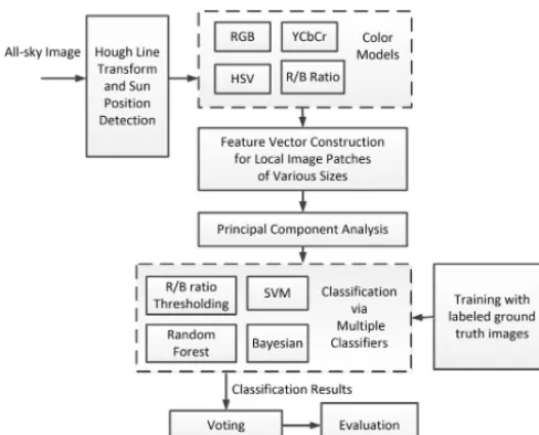
In this paper, we propose to perform cloud detection via extracting features from local image patches with various sizes. Patches of different sizes extract information at dif-ferent levels of resolution. For classification, we utilize mul-tiple supervised learning techniques. We regard the cloud detection problem as a two-class classification problem. In other words, we classify each pixel in the image as cloud or non-cloud. The cloud models are learned through the train-ing process. We consider classifiers includtrain-ing support vec-tor machine (SVM), random forest, and Bayesian classifier. To extract features from each pixel, we calculate the RBR as well as the color components of various color models in-cluding RGB, HSV (hue, saturation, value), and YCbCr. To take advantage of the clues provided by multiple classifiers and multi-level resolution, we employ a scheme to combine multiple classification results to further increase the cloud detection accuracy. The methodology, including the features and the classifiers, is elaborated in Sect. 2. In Sect. 3, the proposed system framework is validated using a set of exper-imental images with manually labeled ground truth. The ex-perimental results using different classifiers are demonstrated and discussed. Finally, conclusions are made in Sect. 4.
2 Methodology
Figure 1.System framework.
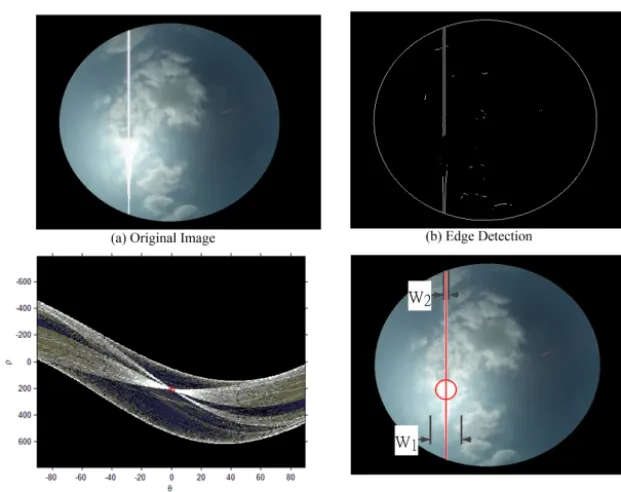
re-parameterizes the line equation as xcosθ+ysinθ=ρ to avoid using the slope parameter for line equation y= mx+b. Because possible values for the slope parameterm range from minus infinity to infinity, it would be infeasi-ble to find the slope parametermvia grid search. After re-parameterizing the line equation, the range of the parameter ρ can be set according to the width and height of the im-age. The range of the parameter θ is from −180◦to 180◦. Figure 2 displays an example of Hough line detection on an image. After detecting the vertical line, the sun position is de-termined by accumulating the intensities of the pixels alongx direction in a window with widthw1. The position with the highest accumulated intensity is the center of the sun. The pixels in the line window with a fixed width w2 are elimi-nated from the image. The pixels within the sun position and the line window with widthw2are determined as non-cloud pixels and do not have to go through the subsequent classi-fication steps. The values of w1andw2 are determined de-pending on the size of the all-sky images. In our experiments, we setw1andw2as 60 and 12 pixels, respectively.
2.2 Color models
RGB is a very common color model, being used in most computer systems. It is an additive color model based on tri-chromatic theory. RGB is easy to implement. However, it is nonlinear with visual perception, and the specification of ors is semi-intuitive. HSV is a color model that describes col-ors in terms of hue, saturation, and value components (Gon-zalez and Woods, 2002). Hue is expressed as a number from 0 to 360◦. The hue component of red starts at 0, green starts at 120, and blue starts at 240. Saturation is the amount of gray in the color. And the value component describes the bright-ness or intensity of the color. YCbCr is a color space used in video and digital photography systems. Y is the luminance
component, and Cb and Cr are the blue-difference and red-difference chroma components. HSV and YCbCr color com-ponents can be obtained from RGB color comcom-ponents using color model transformation equations (Gonzalez and Woods, 2002; Poynton, 2003). Although the color models are not independent and including color components from different color models may introduce redundancy in the feature vector, considering various color models still provides the classifier more information that is beneficial to performing classifica-tion.
2.3 Feature vector construction for local image patches of various sizes
For each pixel, local image patches with various sizes are used to extract features. The size of the image patch at level iisLi×Li,i=1· · ·`, where`denotes the total number of
levels. For each local image patch, the color components and the RBR of all the pixels in the patch are concatenated to form a feature vector. Consequently, the dimension of each feature vector isLi×Li×10. There are ` feature vectors
constructed for each pixel. 2.4 Dimension reduction
We apply principal component analysis (PCA) (Duda et al., 2001) on the feature vectors to reduce their dimensions. Based on the assumption that the importance of the features lies in the variability of the data, PCA chooses principal com-ponents along the directions with the largest variance of the data distribution first. The principal components are a set of new orthogonal bases that can be used to re-express the data in order to reduce the correlation among different variables.
Suppose that the original dataset hasNSamplessamples and each sample hasD1 variables. The data matrixXis estab-lished with each sample as a column vector. Therefore the data matrix X has NSamples columns and D1 rows. If we would like to reduce the feature dimension toD2, then we need to selectD2 principal components. PCA constructs a matrixXTX, which is a matrix proportional to the sample covariance matrix of the datasetX. The first D2 eigenvec-tors ofXTXwhose corresponding eigenvalues are largest are
chosen as principal components. To determine the desired number of dimensionalityD2, we check the eigenvalue ratio Reigenvlaue:
Reigenvalue=
D2 P
k=1
|λk|
D1 P
k=1
|λk|
. (1)
In Eq. (1),λk denotes thekth eigenvalue of XTX. The first
Figure 2.Hough line transform and sun position detection.
2.5 Classifiers 2.5.1 Random forest
Classification and Regression Tree (CART) is a systematic procedure that learns decision trees proposed by Breiman et al. (1984). The splitting rules of the tree include an attribute value test at each node of the tree. Starting from the root node, all training data are used to split the root node. The tree is then built recursively. Considering all the possible splitting rules, CART would construct the tree by selecting the split-ting rule that can maximize the impurity drop when a node is added. The impurity measures the condition of mixed class labels at each node. The goal is to make the class labels at each node as “pure” as possible. The splitting process stops when all the samples in a node have the same class label or when the measure of purity at the child nodes cannot be im-proved compared with its parent node. After a decision tree is built, it might need to be pruned using a cross-validation procedure. The reason for pruning is that some branches of the tree might overfit the training data. In our experiment, we use 10-fold cross validation. Instead of growing a single de-cision tree, random forest grows an ensemble of trees and lets them vote for the most popular class label. In this work, we adopt random split selection (Dietterich, 2000) to build the ensemble of trees. At each node, the split is selected at ran-dom from theK best splits. The features for the split rules are randomly selected. It reduces the correlation between the trees and improves the efficiency of training.
2.5.2 Support vector machine
The SVM learns a set of hyperplanes that maximize the mar-gins between the hyperplanes and the training samples in or-der to lower the classification error of unknown testing sam-ples. The motivation of SVM is that an ideal decision bound-ary should have the largest distance to the nearest training sample of all the classes. However, it might be infeasible to separate data samples using linear hyperplanes in practice. Therefore, soft margins and kernel functions are applied in the SVM in practice. We apply SVM with radial basis func-tions as one of the classifiers in this work. For the details of SVM, please refer to the work by Cristianini and Shawe-Taylor (2000).
2.5.3 Bayesian classifier
Bayesian classifier aims at minimizing the probability of misclassification by classifying a samplex to the class ωk
with the largest posterior probabilityP (ωk|x). Since the
pos-terior probability P (ωk|x) itself is unknown, we need to
transform the problem using the probabilities that can be obtained via training samples. Bayesian classifier uses the Bayes’ theorem to re-express the posterior probability using P (ωk|x)=
P (ωk) P (x|ωk)
P (x) . (2)
In Eq. (2),P (ωk)denotes the prior probability, which is
in-dependent of the testing sample. In other words,P (ωk)states
meteoro-logical conditions and weather forecast report to determine different prior probabilitiesP (ωk)for each day. However, we
use the same prior probabilities for both cloud and non-cloud classes for simplicity, and no meteorological information is required to be involved as prior knowledge in our decision process. The class conditional probabilityP (x|ωk)in Eq. (2)
can be learned from the training samples. We use Gaussian distributions
P (x|ωk)=
1 (2π )p2|6k|
1 2
e−12(x−µk)6k(x−µk)T (3)
to model the class conditional probabilityP (x|ωk)for each
class. In Eq. (3),µkdenotes the mean vector,6kdenotes the
covariance matrix, andpis the number of dimensionality of x andµk, i.e.,x∈ <pandµk∈ <p. To learn the parameters of Gaussian functions, training samples from each class are used to calculate the sample mean vectorµk and the sample covariance matrix 6k for the class. The probability of the
sample P (x)in Eq. (2) does not depend on the class label and can be neglected in the decision process.
2.6 Combining results of multiple-level neighborhoods and classifiers
The concept of a multiple expert system is to take advan-tage of the clues provided by multiple classifiers. Instead of majority voting, we use a different voting scheme to com-bine the results of multiple-level patches and classifiers. The voting is performed in a multi-scale neighborhood, which is inspired by the works of Lowe (2004) and Bay et al. (2008). As shown in Fig. 3, considering a 3×3 neighborhood around a target pixel p at level i, its previous level i−1 and its next level i+1, voting is performed in the scale space of its 3×3×3 neighborhood. That is, we consider the classifier results of a target pixelpitself and its eight neighbors in the 3×3 region at the current leveli, the pixelpand its eight neighbors in the 3×3 region at the previous leveli−1, and the pixelpand its eight neighbors in the 3×3 region at the next leveli+1. For the pixels in leveli−1 in Fig. 3a, the size of the local image patch used for feature vector construction is Li−1×Li−1 in Fig. 3b. Similarly, image patches of size Li×LiandLi+1×Li+1are used for leveliand leveli+1, re-spectively. The voting scheme takes into account the classifi-cation results from four classifiers: RBR thresholding, SVM, random forest, and Bayesian classifier. In other words, there are 27×4 votes for the pixel at each level. LetVcloud(xLeveli)
denotes the number of votes in the neighborhood classified as cloud for pixel x at level i. The decision for a pixel at leveliis determined byVcloud(xLeveli) > Nv. In other words,
if there are more thanNvvotes in the 3×3×3 neighborhood of a pixel at leveli, the pixel is classified as a cloud pixel at this level. Considering the example illustrated in Fig. 3c, the numbers represent the votes in the 3×3×3 neighborhood of pixelp at leveli. Summing up the numbers in Fig. 3c, we obtainVcloud(xLeveli)=61. If the thresholdNvequals to 57,
then pixelp is classified as cloud at leveli. For the bound-ary conditions at level 1 and level`, there is no leveli−1 at level 1, and there is no leveli+1 at level`. There are 18×4 votes for the pixels at these two levels. When performing vot-ing for pixels at level 1 and`, as long as the votes for a pixel exceeds thresholdNv, the pixel is still classified as cloud as that level in our implementation.
To combine the decision at different levels, the probability P (x∈cloud|Num
i=1∼`(xLeveli
∈cloud))is computed. The prob-ability P (x∈cloud|Num
i=1∼`(xLeveli
∈cloud)) states the prob-ability of pixel x belonging to cloud given the number of levels that the pixel is determined as cloud. Suppose Num
i=1∼`(xLeveli
∈cloud)denotes the number of levels at which pixel x is determined as cloud among all levels i=1 to`. If Num
i=1∼`(xLeveli
∈cloud) is 0, it means that the pixel is not classified as clouds in any level. If Num
i=1∼`(xLeveli
∈
cloud) is `, it means the pixel is classified as clouds in all levels. If P (x∈cloud|Num
i=1∼`(xLeveli
∈cloud)) is larger than P (x∈noncloud|Num
i=1∼`(xLeveli
∈cloud)), the final de-cision would classify the pixel to be a cloud pixel. The probabilityP (x∈cloud|Num
i=1∼`(xLeveli
∈cloud)) can be ex-pressed as Eq. (4) using Bayesian rules of conditional proba-bility. In Eq. (4), the termP (Num
i=1∼`(xLeveli
∈cloud))is inde-pendent of class label and would not affect the decision. The prior probabilitiesP (x∈cloud)andP (x∈noncloud)are as-sumed to be equal as stated in Sect. 2.5.3. The likelihood termP (Num
i=1∼`(xLeveli
∈cloud)|x∈cloud)is learned from the training dataset by constructing the normalized histogram of Num
i=1∼`(xLeveli
∈cloud)using all ground truth cloud pixels.
P
x∈cloud|Num
i=1∼` xLeveli
∈cloud
=
P (x∈cloud)P
Num
i=1∼` xLeveli
∈cloud|x∈cloud
P
Num
i=1∼` xLeveli
∈cloud
(4)
3 Experimental results
In this work, the device used to capture the all-sky images is the all-sky camera manufactured by the Santa Barbara In-strument Group (SBIG). The field of view is 185◦. The focal
ac-Figure 3.Voting in the scale space of a 3×3×3 neighborhood:(a)structure of the scale space neighborhood;(b)size of the local image patch at different levels;(c)number of votes in the scale space neighborhood.
curacy, precision, and recall rate. Ten-fold cross validation means that the dataset is divided into 10 none-overlapping subsets. Nine subsets are used for training, and the remain-ing one subset is used for testremain-ing. Then the trainremain-ing sub-sets and testing subsub-sets are rotated for 10 times. The aver-age classification rate of these 10 experiments is the 10-fold cross-validated accuracy. The definitions of detection accu-racy, precision, and recall rate are listed in Eqs. (5) to (7).
Accuracy= TP+TN
TP+TN+FP+FN (5)
Precision= TP
TP+FP (6)
Recall= TP
TP+FN (7)
In Eqs. (5) to (7), true positive (TP) is the number of cloud pixels correctly detected. True negative (TN) is the number of non-cloud pixels that are correctly classified. False pos-itive (FP) is the number of non-cloud pixels that are incor-rectly classified as clouds. False negative (FN) is the number of cloud pixels that are incorrectly classified as non-cloud.
In this work, the RGB thresholding method proposed by Long et al. (2006) will be used as the baseline method for comparison. In Long’s work, an RBR threshold is recom-mended for the whole sky camera and several thresholds are suggested to be used for the total sky imager. Since the desired threshold varies due to different devices and weather conditions, we perform an experiment to test the best threshold for our all-sky camera. Also, to avoid false positive detection at highlighted regions around the sun, we employ an upper bound threshold. Therefore, two thresh-olds, Thrupper and Thrlower, are used in the experiments. A pixel is classified as cloud if its RBR is higher than Thrlower and lower than Thrupper. We perform experiments on sev-eral thresholds to select the best thresholds for our dataset.
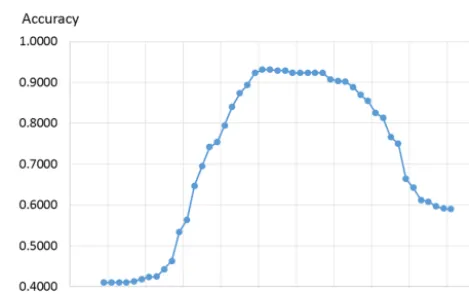
Figure 4.Cloud detection accuracy using various RBR thresholds.
In Fig. 4, we can observe the trade-off between precision and recall. As the thresholds become stricter, the precision increases and the recall drops. Precision rate and recall rate cannot be used alone to measure the accuracy since precision does not consider false negatives and recall does not con-sider false positives. Therefore accuracy defined in Eq. (5) is used as the conclusive metric to measure the performance. As shown in Fig. 4, we have observed that Thrlower=0.8 and Thrupper=0.9 yield the best detection accuracy for our dataset. In the rest of the experiments, we use RBR thresh-olding with Thrlower=0.8 and Thrupper=0.9 as a baseline method for comparison. However, even with the best selected RBR thresholds, the cloud detection result is not satisfy-ing. The thresholds Thrlower=0.8 and Thrupper=0.9 might cause some false positives for certain images while caus-ing some false negatives for other images. Therefore, neither raising or lowering the threshold could improve the detection results by thresholding.
Major-Figure 5.Comparisons of detection accuracy using different classi-fiers with single pixel color information.
ity voting of the four detection methods can yield better ac-curacy. We also compare with the classification accuracy of using only single RGB color model as the feature vector to validate that adding other color models in the feature vector can yield better classification results. With voting schemes that combine the information from multiple classifiers, the accuracy can be enhanced compared with individual single classifiers. However, utilizing only single pixel color infor-mation is not sufficient to give satisfying detection accuracy. Applying features extracted from local image patch is able to further enhance the detection results.
When applying the proposed cloud detection method, we use five levels of local image patches with different sizes, i.e., `=5. The size at each level is L1=5,L2=10,L3=15, L4=20,L5=25. To observe the effect of parameter ThrPCA for dimension reduction at each level, we perform an experi-ment using the feature vector constructed at each single level with SVM as the classifier for different settings of ThrPCA. The value of ThrPCAis typically between 90 and 99 % and is selected empirically. Typically, the accuracy of classifica-tion would increase as the value of ThrPCAgoes from 100 % (which means no dimensionality reduction at all) to 99 %. The accuracy of classification would continue increasing un-til ThrPCA reaches a certain value, which is caused by the benefit of dimensionality reduction. After that, the accuracy of classification would start to decrease due to too much in-formation loss. We plot the cross-validated detection accu-racy in Fig. 6. From Fig. 6, we can observe that the de-tection accuracy at single level using SVM is highest for ThrPCA=97 % at levelsL1andL2. At levelsL3,L4, andL5, the parameter ThrPCA=95 % yields better results. There-fore, for levels L1 and L2, ThrPCA=97 % is selected; for levelsL3,L4, andL5, ThrPCA=95 % is selected.
To combine results of multiple-level patches and classi-fiers, the threshold for votingNvneeds to be determined. The detection accuracy of combining the results using different Nvsettings is plotted in Fig. 7. As shown in Fig. 7, whenNv ranges from 50 to 70, the detection accuracy is higher. We selectNv=57 for the proposed method.
Figure 6. Detection accuracy with different ThrPCA settings in Eq. (5) at each level using SVM.
Figure 7.Detection accuracy with differentNvsettings.
To test the number of levels required to yield better de-tection results, we plot the dede-tection accuracy using different number of levels in Fig. 8. Note that for the sixth level and seventh level, the size of the local image patch isL6=30 and L7=35. We can observe that using four or five levels results in better detection accuracy. When involved with levels with image sizes that are too large, the detection accuracy drops.
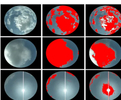
Selected cloud detection results are shown in Fig. 9b. The proposed method using features from multi-scale local image patches can accurately detect clouds in the all-sky images. The pixels within the vertical line and the solar disk would not be detected as clouds even though their intensities are high. The Hough line detection and sun position detection successfully eliminated those pixels before performing clas-sification. Compared with detection results of RBR 0.8–0.9 in Fig. 9c, the proposed method can detect cloud pixels with satisfying accuracy with the proposed multi-level local patch feature extraction mechanism and combination of multiple expert decision.
em-Figure 8.Detection accuracy using different number of levels.
Figure 9.Selected results:(a)original images;(b)detection results of the proposed method;(c)detection results of RBR 0.8–0.9.
ploys dynamic thresholding based on MCE when necessary. The ANN and HYTA methods outperform traditional RBR thresholding. Nevertheless, the accuracy of ANN and HYTA still has room for improvement. Using the single pixel color components described in Sect. 2.2 and utilizing SVM as the classifier can yield slightly improved accuracy compared with ANN and HYTA. Incorporating feature vector extracted from single level 15×15 neighborhood patch can further im-prove the accuracy compared with using only information from single pixel. The proposed method utilizing features ex-tracted from multi-level neighborhood yields the best accu-racy since multiscale information is considered.
4 Conclusions
With the development of all-sky cameras, the cloud condi-tions in the sky can be monitored and useful information can be extracted for solar irradiance prediction with refined spatial and temporal resolutions. Clouds play a critical role
Figure 10.Comparisons of different methods.
in affecting the amount of solar irradiance penetrating the atmosphere. With more accurate cloud detection schemes, subsequent prediction modules that forecast solar irradiance could benefit a lot from the enhanced detection results. In this work, supervised learning methods are utilized to train var-ious classifiers that can distinguish cloud pixels from non-cloud pixels in all-sky images. The classifiers implemented in this work include RBR thresholding, SVM, random for-est, and Bayesian classifier. We propose to use features ex-tracted from multi-level local image patches with different sizes to include local structure and multi-resolution informa-tion. Final decision is made according to multi-level classi-fication results by various classifiers. A challenging dataset with ground truth labels is used to validate the detection schemes. Experiments have also shown that the proposed detection method yields better results than both fixed and dynamic RBR thresholding. Combining the information of multiple classifiers using voting can improve the detection accuracy. It is also validated that using color information in multi-level local neighborhood instead of only a single pixel is very helpful to improve the detection accuracy. To apply the proposed method on different all-sky cameras, images captured by various cameras can be added into the training set to enhance the robustness of the detector. For the selec-tion of parameters ThrPCAandNv for different devices and sites, if the number of levels and feature length are fixed, the desired parameters should not be seriously affected even if the training samples are changed.
5 Data availability
The data are available at https://drive.google.com/open?id= 0B38yagaBviZYNmxReVBIQkVJYkk (Cheng, 2017).
Acknowledgement. The financial support provided by the Ministry of Science and Technology of Taiwan is gratefully acknowledged. Edited by: B. Kahn
References
Bay, H, Ess, A., Tuytelaars, T., and Gool, L. V.: SURF: Speeded Up Robust Features, Comput. Vis. Image Und., 110, 346–359, 2008. Bernecker, D., Riess, C., Christlein, V., Angelopoulou, E., and Hornegger, J.: Representation learning for cloud classification, Lect. Notes Comput. Sc., 8142, 395–404, 2013.
Breiman, L., Friedman, J. H., Olshen, R. A., and Stone, C. J.: Clas-sification and regression trees, Wadsworth & Brooks/Cole Ad-vanced Books & Software, Monterey, CA, USA, 1984.
Calbo, J. and Sabburg, J.: Feature extraction from whole-sky ground-based images for cloud-type recognition, J. Atmos. Ocean. Tech., 25, 3–14, 2008.
Cheng, H. Y.: All-sky Images, National Cen-tral University, https://drive.google.com/open?id= 0B38yagaBviZYNmxReVBIQkVJYkk, last access: 10 Jan-uary 2017.
Cheng, H. Y. and Yu, C. C.: Multi-Model Solar Irradiance Predic-tion Based on Automatic Cloud ClassificaPredic-tion, Energy, 91, 579– 587, 2015a.
Cheng, H.-Y. and Yu, C.-C.: Block-based cloud classification with statistical features and distribution of local texture features, At-mos. Meas. Tech., 8, 1173–1182, doi:10.5194/amt-8-1173-2015, 2015b.
Chow, C. W., Urquhart, B., Lave, M., Dominguez, A., Kleissl, J., Shields, J., and Washom, B.: Intra-hour forecasting with a total sky imager at the UC San Diego solar energy testbed, Sol. En-ergy, 85, 2881–2893, 2011.
Cristianini, N. and Shawe-Taylor, J.: An introduction to support vector machines and other kernel-based learning methods, Cam-bridge University Press, New York, NY, USA, 2000.
Dietterich, T. G.: An Experimental Comparison of Three Methods for Constructing Ensembles of Decision Trees: Bagging, Boost-ing, and Randomization, Mach. Learn., 40, 139–157, 2000. Duda, R. O., Hart, P. E., and Stork, D. G.: Pattern classification, 2nd
edn., John Wiley & Sons, New York, NY, USA, 2001.
Feister, U. and Shields, J.: Cloud and radiance measurements with the VIS/NIR daylight whole sky imager at Lindenberg (Ger-many), Meteorol. Z., 14, 627–639, 2005.
Fu, C. L. and Cheng, H. Y.: Predicting solar irradiance with all-sky image features via regression, Sol. Energy, 97, 537–550, 2013. Gonzalez, R. C. and Woods, R. E.: Digital Image Processing, 2nd
Edition, Prentice Hall, Upper Saddle River, New Jersey, USA, 2002.
Gueymard, C. A.: The sun’s total and spectral irradiance for solar energy applications and solar radiation models, Sol. Energy, 76, 423–453, 2004.
Heinemann, D., Lorenz, E., and Girodo, M.: Solar Irradiance Fore-casting for the Management of Solar Energy Systems, Solar 2006, Denver, CO, USA, 2006.
Heinle, A., Macke, A., and Srivastav, A.: Automatic cloud classi-fication of whole sky images, Atmos. Meas. Tech., 3, 557–567, doi:10.5194/amt-3-557-2010, 2010.
Huo, J. and Lu, D.: Cloud determination of all-sky images under low visibility conditions, J. Atmos. Ocean. Tech., 26, 2172–2180, 2009.
Isosalo, A., Turtinen, M., and Pietikäinen, M.: Cloud characteriza-tion using local texture informacharacteriza-tion, Proc. Finnish Signal Pro-cessing Symp., University of Oulu, Oulu, Finland, 1–6, 2007.
Johnson, R., Hering W., and Shields, J.: Automated visibility and cloud cover measurements with a solid-state imaging system. Tech. Rep., Scripps Institution of Oceanography, Marine Phys-ical Laboratory, University of California, San Diego, USA, SIO Ref. 89-7, GL-TR-89-0061, 128, 1989.
Johnson, R., Shields, J., and Koehler, T.: Analysis and interpretation of simultaneous multi-station whole sky imagery, Scripps Insti-tution of Oceanography, Marine Physical Laboratory, University of California, San Diego, USA, SIO 91-3, PL-TR-91-2214, 1991. Kassianov, E., Long, C. N., and Ovtchinnikov, M.: Cloud sky cover versus cloud fraction: Whole-sky simulations and observations, J. Appl. Meteorol., 44, 86–98, 2005.
Kazantzidis, A., Tzoumanikas, P., Bais, A. F., Fotopoulos, S., and Economou, G.: Cloud detection and classification with the use of whole-sky ground-based images, Atmos. Res., 113, 80–88, 2012. Kubota, M., Nagatsuma, T., and Murayama, Y.: Evening corotat-ing patches: A new type of aurora observed by high sensitiv-ity all-sky cameras in Alaska, Geophys. Res. Lett., 30, 1612, doi:10.1029/2002GL016652, 2003.
Li, Q., Lu, W., and Yang, J.: A Hybrid Thresholding Algorithm for Cloud Detection on Ground-Based, J. Atmos. Ocean. Tech., 28, 1286–1296, 2011.
Li, Z., Cribb, M. C., Chang, F.-L., and Trishchenko, A. P.: Valida-tion of MODIS-retrieved cloud fracValida-tions using whole sky imager measurements at the three ARM sites, Proc. 14th ARMScience Team Meeting, 22–26 March 2004, Albuquerque, NM, USA, At-mospheric Radiation Measurement Program 6, 2–6, 2004. Liu, L., Sun, X., Chen, F., Zhao, S., and Gao, T.: Cloud
Classifica-tion Based on Structure Features of Infrared Images, J. Atmos. Ocean. Tech., 28, 410–417, 2011.
Long, C. N., Sabburg, J., Calbó, J., and Pagès, D.: Retrieving cloud characteristics from ground-based daytime color all-sky images, J. Atmos. Ocean. Tech., 23, 633–652, 2006.
Lorenz, E., Hurka, J., Heinemann, D., and Beyer, H. G.: Irradiance Forecasting for the Power Prediction of Grid-Connected Photo-voltaic Systems, IEEE J. Sel. Top. Appl., 2, 2–10, 2009. Lowe, D. G.: Distinctive image features from scale-invariant
key-points, Int. J. Comput. Vision, 60, 91–110, 2004.
Marquez, M. and Coimbra, C. F. M.: Forecasting of global and di-rect solar irradiance using stochastic learning methods, ground experiments and the NWS database, Sol. Energy, 85, 746–756, 2011.
Marquez, R. and Coimbra, C. F. M.: Intra-hour DNI forecasting based on cloud tracking image analysis, Sol. Energy, 91, 327– 336, 2013.
Martínez-Chico, M., Batlles, F. J., and Bosch, J. L.: Cloud classi-fication in a mediterranean location using radiation data and sky images, Energy, 36, 4055–4062, 2011.
Perez, R., Ineichen, P., Moore, K., Kmiecik, M., Chain, C., George, R., and Vignola, F.: A new operational model for satellite-derived irradiances: description and validation, Sol. Energy, 73, 307–317, 2002.
Perez, R., Kivalov, S., Schlemmer, J., Hemker Jr., K., Renné, D., and Hoff, T.: Validation of short and medium term operational solar radiation forecasts in the US, Sol. Energy, 84, 2161–2172, 2010.
and its impact on surface solar irradiance, J. Appl. Meteorol., 42, 1421–1434, 2003.
Poynton, C.: Digital Video and HDTV: Algorithms and Interfaces, Morgan Kaufmann Publishers, San Francisco, CA, USA, 2003. Remund, J., Perez, R., and Lorenz, E.: Comparison of solar
radia-tion forecasts for the USA, Proc. of the 23rd European PV Con-ference, 1–4 September 2008, Valencia, Spain, 2008.
Roy, G., Hayman, S., and Julian, W.: Sky analysis from CCD im-ages: cloud cover, Lighting Res. Technol., 33, 211–222, 2001. Sabburg, J. and Wong, J.: Evaluation of a Ground-Based Sky
Cam-era System for Use in Surface Irradiance Measurement, J. Atmos. Ocean. Tech., 16, 752–759, 1999.
Shapiro, L. and George, C. S.: Computer Vision, Prentice Books, Upper Saddle River, USA, 2001.
Shields, J., Karr, M., Burden, A., Johnson, R., and Hodgkiss, W.: Continuing support of cloud free line of sight determination in-cluding whole sky imaging of clouds, Final Report for ONR Contract N00014-01-D-0043DO #13, Marine Physical Labora-tory, Scripps Institution of Oceanography, University of Califor-nia, San Diego, USA, Technical Note 273, 2007.
Shields, J., Karr, M., Burden, A., Johnson, R., Mikuls, V., Streeter, J., and Hodgkiss, W.: Research toward Multi-Site Characteri-zation of Sky Obscuration by Clouds, Final Report for Grant N00244-07-1-009, Marine Physical Laboratory, Scripps Institu-tion of Oceanography, University of California, San Diego, USA, Technical Note 274, 2009.
Tapakis, R. and Charalambides, A. G.: Equipment and methodolo-gies for cloud detection and classification: A review, Sol. Energy, 95, 392–430, 2013.
West, S. R., Rowe, D., Sayeef, S., and Berry, A.: Short-term irra-diance forecasting using skycams: Motivation and development, Sol. Energy, 110, 188–207, 2014.
Wood-Bradley, P., Zapata, J., and Pye, J.: Cloud tracking with opti-cal flow for short-term solar forecasting, 50th conference of the Australian Solar Energy Society, Melbourne, Australia, Decem-ber, 2012.