Transmuted Modified Inverse Weibull distribution:
Properties and application
Muhammad Shuaib Khan
School of Mathematical and Physical Sciences
The University of Newcastle, Callaghan, NSW 2308, Australia Email: muhammad.s.khan@newcastle.edu.au
Abstract
This paper examines the potential usefulness of the transmuted modified inverse Weibull distribution. The four-parameter model holds eleven lifetime distributions as special cases. Some theoretical properties of the transmuted modified inverse Weibull distribution are studied; which includes the quantile, median, entropy, mean deviations, mean, geometric mean and harmonic mean. The estimation is obtained by using the method of maximum likelihood. An application to real dataset is provided to show the better fit of the transmuted modified inverse Weibull distribution.
Keywords: Reliability functions; mean; geometric mean; harmonic mean; entropy; maximum likelihood estimation.
1. Introduction
In the field of reliability, the well-known inverse Weibull family of distributions has proved to be of considerable interest in modeling various mechanism with instantaneous failure rates. Elbatal (2013) introduced and studied the transmuted modified inverse Weibull distribution and formulated some of its mathematical properties. This paper investigates the potential usefulness of the transmuted modified inverse Weibull distribution for analyzing survival data. This paper presents the visualization of the density function and instantaneous failure rate function for some selected values of parameters. The subject model has the flexibility to approach eleven different lifetime distributions. The quadratic rank transmuted map (QRTM) technique was used to develop the transmuted modified inverse Weibull distribution in order to generate a flexible lifetime model. Many researchers have proposed transmuted family of lifetime distributions by using QRTM technique such as: transmuted Weibull distribution by Gokarna el al. (2011), the transmuted modified Weibull distribution by Khan and King (2013), the transmuted inverse Weibull distribution by Khan, King and Hudson (2014a) and Khan and King (2014b), Elbatal el al. (2014) proposed the transmuted exponentiated Frechet distribution with Applications and the transmuted G-family of distribution was introduced by Bourguignon et al. (2016). This paper focuses on the mathematical properties of the transmuted modified inverse Weibull distribution along with its reliability behavior. Khan and King (2012) introduced and developed the modified inverse Weibull distribution. The random variable has the modified inverse Weibull distribution, if its cumulative distribution function (cdf) is given by
1 ( ; , , ) exp
F t
t t
= − −
2
= . It coincides with the modified inverse exponential distribution for =1. A random variable T is said to have transmuted distribution if its cumulative distribution function (cdf) is given by
(
)
2( ) 1 ( ) ( ) , 1
F t = + G t −G t (2)
and
(
)
( ) ( ) 1 2 ( ) ,
f t =g t + − G t (3)
whereG t( )is the cdf of the baseline model. Elbatal (2013) introduced the transmuted modified inverse Weibull distribution by using the quadratic rank transmutation map technique pioneered by Shaw et al. (2009). The article is organized as follows, Section 2 presents the flexibility of the transmuted modified inverse Weibull distribution and special sub-models. Section 3 demonstrates a range of mathematical properties, which includes quantile functions, mean deviation, entropy, mean, geometric mean and harmonic mean. The maximum likelihood estimates (MLEs) and the asymptotic confidence intervals of the unknown parameters are presented in Section 4. In Section 5, a real lifetime dataset is analyzed to show the flexibility of the transmuted modified inverse Weibull distribution. Finally, some concluding remarks are given in Section 6.
2. Transmuted modified Inverse Weibull distribution
Consider a system with lifetime Tfollow the transmuted modified inverse Weibull distribution with parameters 𝛼, 𝛽, 𝛾 > 0, |𝜆| ≤ 1 and 𝑡 > 0. The probability density function is defined as
( )
1 2
1 1 1 1
( ; , , , ) 1 2 λ
β β β
α α
f t = α + βγ exp γ + λ exp γ
t t t t t t
−
− − − − −
(4)
The cumulative distribution function (cdf) for t is given by
( )
1 1
( ; , , , ) 1 λ
β β
α α
F t = exp γ + λ exp γ
t t t t
− − − − −
, (5)
where 𝛼 and 𝛾 are the scale parameters and 𝛽 is a shape parameter and λ is the transmuted parameter of the transmuted modified inverse Weibull distribution. If the random variable
𝑇 has a pdf (4), then it can be denoted as 𝑇~TMIW(𝛼, 𝛽, 𝛾, 𝜆). The TMIW distribution contains several lifetime models which are widely used in reliability theory listed in Table 1. The flexibility of the transmuted modified inverse Weibull distribution is explained in table 1. The reliability function (RF) of the transmuted modified inverse Weibull distribution is denoted by 𝑅(t) also known as the survivor function defined as
( )
1 1
( ; , , , ) 1 1 λ
β β
α α
R t = exp γ + λ exp γ
t t t t
− − − − − −
. (6)
( )
( )
1 2
1 1 1 1
1 2 λ
( ; , , , ) .
1 1
1 1 λ
β β β
β β
α α
α + βγ exp γ + λ exp γ
t t t t t t
h t =
α α
exp γ + λ exp γ
t t t t
−
− − − − −
− − − − − −
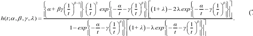
(7)
The reversed hazard function is quite popular in distribution theory. The reversed hazard function for the transmuted modified inverse Weibull distribution also known as failure rate denoted by 𝑟(𝑡) defined as
(
)
(
)
1 2
1 1 1
1 2 λ
( ; , , , ) .
1
1 λ
β β
β α
α + βγ + λ exp γ
t t t t
r t =
α
+ λ exp γ
t t
−
− − −
− − −
(8)
Table 1: Transmuted modified inverse Weibull sub-models
S. No Distribution TMIW
1 TMIE 1
2 TMIR 2
3 MIW 0
4 MIR 2 0
5 MIE 1 0
6 TIW 0
7 TIR 0 2
8 TIE 0 1
9 IW 0 0
10 IR 0 2 0
11 IE 0 1 0
Note: T, Transmuted; M, Modified; I, Inverse; W, Weibull; E, Exponential; R, Rayleigh
The TMIW distribution includes as special cases: the transmuted modified Inverse exponential, transmuted modified Inverse Rayleigh, Modified Inverse Weibull, Modified Inverse Rayleigh and Modified Inverse exponential distributions. Fig. 1 shows the transmuted modified inverse Weibull pdf for some selected values of parameters. The Cumulative hazard function (CHF) of the transmuted modified inverse Weibull distribution is denoted by 𝐻(𝑡) defined as
(
)
1 1
( ; , , , ) ln 1 λ .
β β
α α
H t = exp γ + λ exp γ
t t t t
− − − − − −
(9)
Figure 1: Transmuted modified inverse Weibull pdf
3. Statistical Properties
This section explains some basic statistical properties of the TMIW(𝛼, 𝛽, 𝛾, 𝜆) distribution, such as quantile and median, mean, geometric mean, harmonic mean, mean deviations and Rényi entropy.
3.1 Quantile and median
The quantile 𝑡𝑞 of the TMIW(𝛼, 𝛽, 𝛾, 𝜆) is the real solution of the following equation
2
1 2λ
ln 0.
1 1 4λ 1
β
q q
α
γ + + =
t t ( + λ) ( + λ) ( q)
− − −
(10)
The above equation (10) has no closed form solution in 𝑡𝑞, so we have different cases by substituting the parametric values in the above quantile equation. The q-th quantile of the
TMIR(𝛼, 𝛾, 𝜆) can be obtained by substituting 𝛽 = 2
(
) (
)
(
)
2
2
2γ
.
2λ 4 γ ln
1 1 4λ 1
q
t =
α+ α
+ λ + λ q
− −
− − −
By substituting q= 0.5 in equation (10), we obtain the median of the TMIW(𝛼, 𝛽, 𝛾, 𝜆). The median life of the transmuted modified inverse Weibull distribution is the 50th percentile. In practical this is the life by which 50% of the units will be expected to have failed and therefore it is the life at which 50% of the units would be expected to still survive.
3.2 Mean Deviations
The degree of scatter in a population is widely measured by the totality of deviations from the mean and median. If 𝑇 has the transmuted modified inverse Weibull distribution, then the mean deviation about mean 𝜇 = 𝐸(𝑇) and about the median M can be obtained from the following equations
) ( ) (
1
= F − , 2=−2(M) (11)
The mean 𝜇 = 𝐸(𝑇) is obtained from equation (11) and the median M is the solution of the non-linear equation, where 𝜓(𝑎) can be obtained as
(
)
1 ( 1)0 0
( 1) ( 1, ) ( 1) ( ( 1), )
( ) 1 2
! !
i i i i i i
i i
i a i a
a
i i
− + − +
= =
− + − +
= + + −
( 1 1) 1 ( 1) ( )1
0 0
( 1) 2 ( 1, ) ( 1) 2 ( ( 1), )
! !
i i i
i i i i i i
i i
i a i a
i i − − − − + − + − + + = = − + − + +
(12)where
( )
,t =0tw−1e−wdw for(
0)
is the incomplete gamma function. Hence, the measure in equation (11) can be obtained from equation (12). The quantity 𝜓(𝑎) can also be used to find Bonferroni and Lorenz curves which have applications in econometrics and finance. They are given by( )
p q PB = ( ),
( )
(q)
P L =
where q=Q
( )
P is calculated from equation (5) for a given probability 𝑃.3.3 Entropy
The entropy of a random variable T with density f (t) is a measure of variation of the uncertainty. A large value of the entropy shows the greater uncertainty in the data. The Rényi entropy is defined as
1
( ) log ( )
1
R
I f t dt
=
−
where 0and 1. The integral in IR() of the TMIWD(𝑡, 𝛼, 𝛽, 𝛾, 𝜆) can be defined as
(
)
− − + + = 0 2 1 0 2 1 1 1 )( W W dt
t t
dt t
f
where − − = t t
W exp 1
(
)
− = + − + + − + = 0 2 1 0 1 ln ) ( exp 1 1 1 2 ) 1 ( 1 dt W j t t j j j jj
Finally the above integral reduces to
(
)
(
)
= + + + − + = 0 , , 1 2 ! ) 1 ( 1 k j i k k j i k j j i jk
(
)
( )(
)
( )
2 1
1 2 + + − +
+ − + + i k i j i k i
, , 0
1 ( 1) 2
( ) log (1 ) log
1 1 ! 1
i j
j k
R
i j k I j i k + = − = + + − −
+ (
)
(
)
( )(
)
(
)
2 1 2 1i k i
k k
j i k i
j + + − + + + + − +
(13)
3.4 Mean, Geometric mean and harmonic mean
For a random variable 𝑇 with density (4) for the TMIW distribution then it can be formulated for mean as follows
( ) 1 2 ( )
0
1 1 1 1
1 2 λ
β β β
α α
E t = t α + βγ exp γ + λ exp γ dt
t t t t t t
− − − − − −
The above expression reduces to ( ) ( )
0 0
1 1 1 1
1
β β
α α
E t = + λ α exp γ dt βγ exp γ dt
t t t t t t
− − + − −
0 01 2 1 1 2 1
2 2 2
β β
α α
α exp γ dt βγ exp γ dt
t t t t t t
− − − + − −
the above integral simplified to
( ) ( ) ( ) 1 ( ) ( )1
0 0 0 0
1 1
1
! !
i i i i
i i
i i
α α
E t = + λ α t exp dt βγ t exp dt
i t i t
− + − − = = − − − + −
( ) 1 ( ) ( 1)
0 0 0 0
2 2 2 2
2
! !
i i i i
i i
i i
α α
α t exp dt βγ t exp dt
i t i t
− − − + = = − − − − + −
.the above integral reduces to the first moment of the TMIW distribution
( ) ( ) 1 ( ) ( ) 1 ( 1) ( )
(
( ))
0 0
1 1
1 1 1
! !
i i i i
i i
i i
E t = + λ α i α βγ i
i i − + − = = − − + + −
( ) ( ) ( ) ( ) ( )(
( ))
1 1 2 1 1 0 0 2 22 1 1
2 ! 2 !
i i i i i
i
i i
i i
α α
i βγ i
i i − + − + −+ + = = − − − + + −
. (14) For non-negative random variable 𝑇 with density (4) for the TMIW distribution could be formulated geometric mean as follows
( ) 1 2 ( )
0
1 1 1 1
log 1 2 λ
β β β
α α
G = t α + βγ exp γ + λ exp γ dt
t t t t t t
− − − − − −
.( ) ( ) 2 ( ) 1
0 0
1 1 1 1
1 log log
β β
α α
G = + λ α t exp γ dt βγ t exp γ dt
t t t t t t
+ − − + − −
( ) 2 ( ) 1
0 0
1 2 1 1 2 1
2 log 2 log 2
β β
α α
α t exp γ dt βγ t exp γ dt
t t t t t t
+ − − − + − −
.By solving the exponent, the above integral reduces to
( ) ( ) ( ) 2 ( ) ( ) ( 1)1
0 0 0 0
1 1
1 log log
! !
i i i i
i i
i i
α α
G = + λ α t t exp dt βγ t t exp dt
i t i t
− + − − − = = − − − + −
( ) ( ) 2 ( ) ( ) ( 1) 1
0 0 0 0
2 2 2 2
2 log log
! !
i i i i
i i
i i
α α
α t t exp dt βγ t t exp dt
i t i t
− − − + − = = − − − − + −
.By using the 𝑛𝑡ℎ order derivative of gamma function is given by
( ) ( )
(
( ) ( 3)( ))
( )(
( ) ( ( 1) 2)( ))
0 0
1 1
1 log 1 log 1
! !
i i i i
i i
i i
G = + λ α βγ
i i − + − − − = = − − + + +
( )
(
( ) ( 3)( ))
( )(
( ) ( ( )1 2)( ))
0 0
2 2
2 log 2 1 log 2 1
! !
i i i i
i i i i α βγ i i − − − + − = = − − − + + +
.(15) For a random variable 𝑇 with density (4) for the TMIW distribution then it can be formulated for harmonic mean as follows( )
1 2
0
1 1 1 1 1 1
1 2 λ
β β β
α α
= α + βγ exp γ + λ exp γ dt
H t t t t t t t
− − − − − −
The above expression reduces to
( ) 3 2
0 0
1 1 1 1 1
1
β β
α α
= + λ α exp γ dt βγ exp γ dt
H t t t t t t
+ − − + − −
3 2 0 01 2 1 1 2 1
2 2 2
β β
α α
α exp γ dt βγ exp γ dt
t t t t t t
+ − − − + − −
By solving the exponent, the above integral simplified to
( ) ( ) 3 ( ) ( 1) 2
0 0 0 0
1 1
1 1
! !
i i i i
i i
i i
α α
= + λ α t exp dt βγ t exp dt
H i t i t
− + − − − = = − − − + −
( ) 3 ( ) ( 1) 2
0 0 0 0
2 2 2 2
2
! !
i i i i
i i
i i
α α
α t exp dt βγ t exp dt
i t i t
− − − + − = = − − − − + −
.Finally, the above integral simplified to harmonic mean as
( ) 2 ( ) ( ) ( 1) 1 ( )
(
( ))
0 0
1 1
1
1 2 1 1
! !
i i i i
i i
i i
= + λ α i α βγ i
H i i
( ) ( ) ( )
( ) ( )
(
( ))
1 1 1
2 1 1
0 0
2 2
2 2 1 1
2 ! 2 !
i i i i i
i
i i
i i
α α
i βγ i
i i − +− − + ++ − = = − − − + + + +
. (16)
One can easily compute these integrals numerically in software such as R and SAS languages to obtain the mean, geometric mean and harmonic mean.
4. Maximum Likelihood Estimation
Consider the random samples t1,t2,...tn consisting of nobservations from the transmuted modified Inverse Weibull distribution. Then from (4), the log-likelihood function is given by
( )
11 1 1 1 1
1 1 1 1 1
ln ln 2 ln ln 1 2λ
β β β
n n n n n
i= i i= i i= i i= i i= i i
α
L = α+ βγ + α γ + + λ exp γ
t t t t t t
− − − − − −
(17) By differentiating ln Lwith respect to α,β,γ andλ, the likelihood equations are obtained as follows1
1 1 1
1 1
2λ
ln 1 1
0
1 1
1 2λ
β
n n n i i i
β β
i= i= i i=
i i i
α
exp γ
t t t
L
= + =
α t α
α + βγ ( + λ) exp γ
t t t
− − − − − − −
(18)1
1
1 1
1 1 1 1 1
ln 1 2 exp ln
ln 1 1
ln 1 1 1 2λexp β β β β n
i i i i i i
β β
i= i i i=
i i i
α
γ β + λγ γ
t t t t t t
L
= γ +
β t t α
α+ βγ ( + λ) γ
t t t
− − − − − − − −
1 0 n n i= =
(19)
1
1
1 1 1
1 1
1 2λ exp
ln 1 0 1 1 1 2λexp β β β β
n n n i i i
i
β β
i= i= i i=
i i i
α γ
β t t t
t L
= + =
γ t α
α+ βγ ( + λ) γ
t t t
− − − − − − − −
(20)1
1 1 2 exp
ln
0 1
1 2λexp
β
n i i
β i= i i α γ t t L = = α ( + λ) γ t t − − − − − −
By solving equations (18), (19), (20) and (21), these solutions will yield the ML estimators γ
, β ,
αˆ ˆ ˆ andλˆ. These equations can be solved through numerical iterative method by using the R package (2013). For the transmuted modified inverse Weibull distribution pdf all the second order derivatives are exist. Thus, the observed information matrix is
2 2 2 2
2
2 2 2 2
2 1
2 2 2 2
2
2 2 2 2
2
ln ln ln ln
ln ln ln ln
ln ln ln ln
ln ln ln ln
L L L L
L L L L
V E
L L L L
L L L L
−
= −
(22)
By solving this observed information matrix, these solutions will yield the asymptotic variance and co-variances of these ML estimators for αˆ,βˆ,γˆ andλˆ. By using (22), approximately the 100 1( −)%approximate confidence intervals for the parameters α,β,γ,λ
can be determined as
/2 ˆ11
ˆ
α ± Z V , β ± Zˆ /2 Vˆ22 , γ ± Zˆ /2 Vˆ33 ,λ ± Zˆ /2 Vˆ44 (23) where Z/ 2 is the upperth percentile of the standard normal distribution.
5. Data Analysis
This section provides the data analysis to assess the goodness-of-fit of the TMIW distribution with respect to survival remission times (in months) of bladder cancer data to see how the subject model works in practice. The data have been obtained from Lee and Wang (2003, p. 231): 0.08, 2.09, 3.48, 4.87, 6.94, 8.66, 13.11, 23.63, 0.20, 2.23, 3.52, 4.98, 6.97, 9.02, 13.29, 0.40, 2.26, 3.57, 5.06,7.09, 9.22, 13.80, 25.74, 0.50, 2.46, 3.64, 5.09, 7.26, 9.47, 14.24, 25.82, 0.51, 2.54, 3.70, 5.17, 7.28, 9.74, 14.76, 26.31, 0.81, 2.62, 3.82, 5.32, 7.32, 10.06, 14.77, 32.15, 2.64, 3.88, 5.32, 7.39, 10.34, 14.83, 34.26, 0.90, 2.69, 4.18, 5.34, 7.59, 10.66, 15.96, 36.66, 1.05, 2.69, 4.23, 5.41, 7.62, 10.75, 16.62, 43.01, 1.19, 2.75, 4.26, 5.41, 7.63, 17.12, 46.12, 1.26, 2.83, 4.33, 5.49, 7.66, 11.25, 17.14, 1.35, 2.87, 5.62, 7.87, 11.64, 17.36, 1.40, 3.02, 4.34, 5.71, 7.93, 11.79, 18.10, 1.46, 4.40, 5.85, 8.26, 11.98, 19.13, 1.76, 3.25, 4.50, 6.25, 8.37, 12.02, 2.02, 3.31, 4.51, 6.54, 8.53, 12.03, 20.28, 2.02, 3.36, 6.76, 12.07, 21.73, 2.07, 3.36, 6.93, 8.65, 12.63, 22.69.
Table 2: MLEs of the Parameters for the TMIW, MIW, MIR, TIR and TIE models for bladder cancer data set.
Model
MLE of the Parameters AIC BIC
ˆ ˆ ˆ ˆ
TMIW 0.0168 (0.7531)
0.7562 (0.0477)
2.4179 (0.5807)
0.0011 (0.4188)
881.69 893.07
MIW 2.4659 (0.2188)
1.5692 (1.2335)
0.0079 (2.0208)
TIR TIE
-
-
-
-
0.6125 (0.0546)
2.4659 (0.4323)
0.0002 (0.0970)
0.0013 (0.3232)
1526.87
909.05
1532.56
914.75
Figure 3: Histogram of the data verses fitted models
The MLEs of the unknown parameters are obtained for these models namely: Transmuted modified Inverse Weibull (TMIW), Modified Inverse Weibull (MIW), Modified Inverse Rayleigh (MIR) Transmuted Inverse Rayleigh (TIR) and Transmuted Inverse Exponential (TIE) distributions and results are displayed in Table 2. The MLEs of the parameters with their corresponding standard errors are given in parenthesis with their corresponding the Akaike information criteria (AIC) and Bayesian information criterion (BIC) for the fitted models are given in Table 2. To compare the TMIW distribution with other four lifetime distributions, I also consider the K-S test, Cramérvon Mises, and Anderson-Darling goodness-of-fit statistics displayed in Table 3. According to these goodness of-fit tests in table 3 shows that the TMIW distribution gives a better fit than the other four distributions for bladder cancer data.
Table 3: The Cramér-von Mises and Anderson-Darling goodness of-fit tests
Model K-S test 𝒲 𝒜
TMIW 0.1451 0.7774 4.7671
MIW 0.2320 1.1446 6.8039
MIR 0.2319 1.1445 6.8038
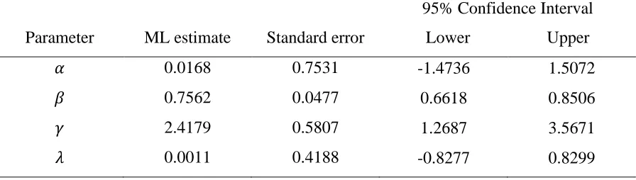
Using the maximum likelihood estimates of the unknown parameters, the approximately 95% two-sided confidence interval for the parameters displayed in Table 4. Hence the data points from the transmuted modified Inverse Weibull (TMIW) has better relationship with remission times of bladder cancer data and could be an appropriate model for fitting survival data.
Table 4: Estimated Parameters of the TMIW distribution with 95% confidence interval
95% Confidence Interval Parameter ML estimate Standard error Lower Upper
𝛼 0.0168 0.7531 -1.4736 1.5072
𝛽 0.7562 0.0477 0.6618 0.8506
𝛾 2.4179 0.5807 1.2687 3.5671
𝜆 0.0011 0.4188 -0.8277 0.8299
6. Conclusion
This paper studied the transmuted modified inverse Weibull distribution and formulated some of its theoretical properties. It is seen that the TMIW distribution has several desirable properties and numerous existing well-known distributions. From the instantaneous failure rate analysis, it is seen that it has increasing and decreasing failure rate pattern for lifetime data. From data analysis it concludes that the TMIW distribution yields an improved fit than the other four lifetime distributions.
References
1. Aryal. Gokarna R., Tsokos. Chris P. (2011). Transmuted Weibull Distribution: A Generalization of the Weibull Probability Distribution. European Journal of Pure and Applied Mathematics, 4 (2), 89-102.
2. Bourguignon, M., Ghosh, I., and Cordeiro, G. M. (2016). General Results for the Transmuted Family of Distributions and New Models, Journal of Probability and Statistics, Vol. 2016, Article ID 7208425, 12 pages, http://dx.doi.org/10.1155/2016/7208425.
4. Elbatal. I., Asha. G and Raja. A Vincent. (2014). Transmuted Exponentiated Frechet Distribution: Properties and Applications. J. Stat. Appl. Pro. 3 (3), 379-394. 5. Khan, M.S, Robert King. (2012). Modified Inverse Weibull Distribution J. Stat.
Appl. Pro. 1 (2), 115-132.
6. Khan, M.S, King Robert. (2013). Transmuted Modified Weibull Distribution: A Generalization of the Modified Weibull Probability Distribution, European Journal of Pure And Applied Mathematics, 6 (1), 66-88.
7. Khan, M. S., King. R., and Hudson I. L. (2014a). Characterizations of the transmuted Inverse Weibull distribution, ANZIAM J. Vol. 55 (EMAC2013), C197–C217.
8. Khan M. Shuaib and King Robert. (2014b). A New Class of Transmuted Inverse Weibull Distribution for Reliability Analysis, American Journal of Mathematical and Management Sciences, 33 (4), 261-286.
9. Khan, M.S. (2014). Modified Inverse Rayleigh Distribution. International Journal of Computer Applications, 87 (13), 28–33, February 2014.
10. Lee, E. T.,Wang, J.W. (2003). Statistical Methods for Survival Data Analysis. 3rd ed. New York:Wiley.
11. Merovci, F. (2013). Transmuted Rayleigh distribution. Austrian Journal of Statistics. 42 (1): 21-31.
12. Oguntunde PE, Adejumo AO. (2015). The transmuted inverse exponential distribution. Int J Adv Stat Probab. 3 (1), 1–7.
13. R Development Core Team. (2013). A Language and Environment for Statistical Computing, R Foundation for Statistical Computing. Vienna, Austria.
14. Sharma VK, Singh SK, and Singh U. (2014). A new upside-down bathtub shaped hazard rate model for survival data analysis, Applied Mathematics and Computation, 239, 242–253.