An overview on robust design hybrid metamodeling: Advanced methodology in process optimization under uncertainty Pages 1-32 Download PDF

(1)

International Journal of Industrial Engineering Computations 9 (2018) 1–32

Contents lists available at GrowingScience

International Journal of Industrial Engineering Computations

homepage: www.GrowingScience.com/ijiec

An overview on robust design hybrid metamodeling: Advanced methodology in

process optimization under uncertainty

Amir Parnianifarda*_{, A.S. Azfanizam}a_{, M.K.A. Ariffin}a_{and M.I.S. Ismail}a

a_{Department of Mechanical and Manufacturing Engineering, Faculty of Engineering, Universiti Putra Malaysia, 43400 UPM Serdang,}

Selangor, Malaysia

C H R O N I C L E A B S T R A C T

Article history:

Received January 15 2017 Received in Revised Format April 1 2017

Accepted May 20 2017 Available online May 26 2017

Nowadays, process optimization has been an interest in engineering design for improving the performance and reducing cost. In practice, in addition to uncertainty or noise parameters, a comprehensive optimization model must be able to attend other circumstances which might be imposed in problems under real operational conditions such as dynamic objectives, multi-responses, various probabilistic distribution, discrete and continuous data, physical constraints to design parameters, performance cost, computational complexity and multi-process environment. The main goal of this paper is to give a general overview on topics with brief systematic review and concise discussions about the recent development on comprehensive robust design optimization methods under hybrid aforesaid circumstances. Both optimization methods of mathematical programming based on Taguchi approach and robust optimization based on scenario sets are briefly described. Metamodels hybrid robust design is discussed as an appropriate methodology to decrease computational complexity in problems under uncertainty. In this context, the authors’ policy is to choose important topics for giving a systematic picture to those who wish to be more familiar with recent studies about robust design optimization hybrid metamodels, also by attending real circumstances in practice. In particular, production and project management are considered as two important methodologies that could be improved by applications of advanced robust design combining with metamodel methods.

Robust design Metamodeling Uncertainty Process optimization

1. Introduction

(2)

: , 1,2, … ,

(1)

subject to:

0, 1,2, … ,

where shows the objectives set (single or multi) and , illustrate the set of inequality and quality constraints (Beyer & Sendhoff, 2007). In particular, there are a number of mathematical formulations in literature which try to find optimum and feasible solution using constraints. Some of them are Linear Programming (LP), Mixed Integer Programming (MIP), Second Order Cone Programming (SOCP), and Semidefinite Programming (SDP) problems.

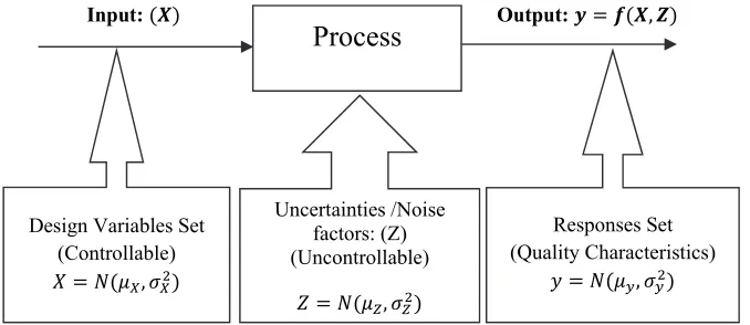
In practice, most processes have been faced by uncontrollable parameters as uncertainties and noise factors which affect on process performance.A general overview of the process is illustrated in Fig. 1. In process quality approach a process consists of three main parts which are design variables (controllable), uncertainties or noise factors (uncontrollable), and quality characteristics (responses). This is the duty of design engineer to identify what is input, what is output and what is an ideal function for designing the process (Phadke, 1989). Such a considering uncertainty or noise parameter in the process leads to introduce Robust Design Optimization (RDO) methods. The term of robust design has been attached by Genichi Taguchi as a pioneer in the word of robust design philosophy (Park, 1996; Park & Antony, 2008; Phadke, 1989). According to Park (1996) robust design is an engineering methodology for optimizing the product and process conditions which are minimally sensitive to the various causes of variation, and that produce high-quality products with low development and designing costs. Ben-Tal et al. (2009) mentioned that the data of real world optimization problems more often are uncertain and not identified exactly when the problem is being solved. The reasons for uncertainty in data are classified in some parts. The first part is to measurement or estimation errors which arise from the impossibility to estimate the exact data on characteristics of physical processes. Second, implementation errors arising from the impossibility to implement an exact solution as it is estimated before. In real word optimization problems, it is desirable to consider the possibility of shifting the problem into meaningless due to the existence of even a small uncertainty. Furthermore, due to adding uncertainties and noise factors into the model, the computational complexity in design problems have incresed in engineering design. The expensive analysis and simulation processes are due to computation burden which caused by the physical or computer testing of data. Approximation or metamodeling techniques have been often used to address such a challenge. Various engineering disciplines including statistics, mathematics, computer science have been employed to develop metamodeling techniques (Wang & Shan, 2007). Metamodeling techniques have been used to avoid intensive computational and numerical analysis, which might squander times and resource for estimating model's parameters especially under uncertain or noisy

Process

Design Variables Set (Controllable)

,

Uncertainties /Noise factors: (Z) (Uncontrollable)

,

Responses Set (Quality Characteristics)

,

Input: Output: ,

Fig. 1. An overview of process that shows Input, Output, and Uncertainties sets

(3)

A. Parnianifard et al.

conditions. This study contributes to present an analytical review of references to offer a comprehensive viewpoint related to a particular field of interest. In addition, it is to identify lack of attention to particular areas of research.

2. The proposed method

The main purpose of literature review is to identify, evaluate and interprete most relevant available studies related to the particular field of research. Our strategy for collecting, reviewing and analyzing resources in literature is mentioned as three phases:

i. As primary sources, five electronic databases were attended to collect relevant studies. The electronic databases which applied in search process are listed in Table 1.

Table 1

Electronic source (database)

Electronic Source URL

Science Direct http://sciencedirect.com/

Springer Link http://link.springer.com/

Wiley http://onlinelibrary.wiley.com/

IEEE Xplore http://ieeexplore.ieee.org/

Google Scholar https://scholar.google.com/

ii. Different keywords and their combinations were used to search relevant resources in literature from mentioned electronic databases. Note that, this context is focused for illustrating the recent development of robust design optimization particulary with employing metamodels and its application in two different types of relevant processes in management science consist of production management and project management. Moreover, a certain combination of keywords was used to filter results, which are “Robust design Optimization”, “Robust Metamodel(ing)”, and Process Optimization” with using the conjunction ‘AND’ by each term of ‘under Uncertainty”, or ‘Noise Factors”. Notably, references which mentioned in some relevant literature review could be employed to recognize some appropriate articles.

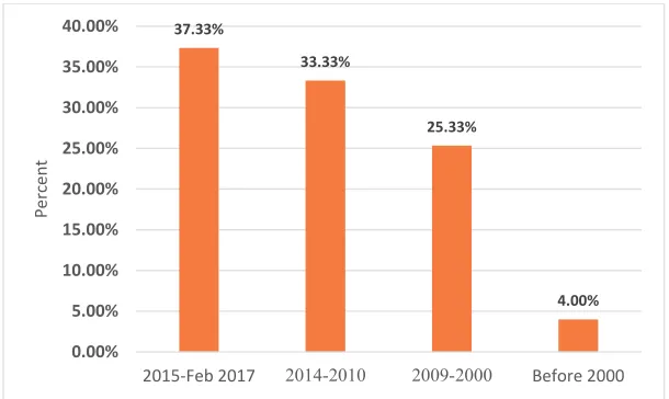
iii. Totally, our findings consist of above 500 different resources in the literature. Based on abstract and conclusion which are associated with interesting topics, 150 articles were filtered. The magnitude (percent) of total articles based on published year is shown in Fig. 2, and as can be seen from the figure, the time period for the most proportion of reviewed resources was belonged to recent years to ensure up-to-date resources included.

Fig. 2. Filtered articles based on published year - total: 150 articles

37.33%

33.33%

25.33%

4.00%

0.00% 5.00% 10.00% 15.00% 20.00% 25.00% 30.00% 35.00% 40.00%

2015‐Feb 2017 2014-2010 2009-2000 Before 2000

Pe

rc

e

n

(4)

Totally, our findings were consist of above 500 different resources in the literature. Based on abstract and conclusion which are associated with interesting topics, 150 articles were filtered. The magnitude (percent) of total articles based on published year is shown in Fig. 2, and as can be seen from the figure, the time period for the most proportion of reviewed resources belongs to recent years to ensure up-to-date resources included. For each article, an in-depth review was done and analytical results were gathered in the same database. Extracted information was defined based on two different terms included objective and methodology. Relevant extracted information are analytically discussed in section 4.

This paper is organized as follows. In section 2, the review strategy and procedure are described. Section 3 provides some general information about the relevant topics. The systematic findings and results which have been achieved by review resources are explained in section 4. Finally, the paper is concluded in section 5.

3. Basic information

Process optimization is the discipline of adjusting a process to optimize some specified set of parameters without violating some constraints. The most common goals are minimizing cost and maximizing throughput and/or efficiency. When optimizing a process, the goal is to maximize one or more of the process specifications, while keeping all others within their constraints. In real world, to achieve an accurate solution in model, we need to consider some circumstances in designing and modeling a process. In practice a process definitely has been affected by most external and environmental uncertainty or noise factors (Ben-Tal et al., 2009) that cause to response quality specifications be far from ideal points and have variances. In addition, each process has to coincide itself to be softly compatible with changing in its condition to keep flexibility and reduce extra cost which might impose to process for adjusting with new conditions (Ehrgott et al., 2014; Haobo et al., 2015). For instance, in the relevant process in management science, customer needs (Gasior & Józefczyk, 2009), external diplomatic rules, economical pressure, local and global environmental policies (Geletu & Li, 2014) and managing rules can be changed over time and it changes the process goals and ideal points of responses. So, it is the duty of engineers to design flexible processes which can be adjusted immediately coincide to new circumstances as soon as possible. Robust design optimization methodology plays an important role to develop high reliability in the process (Bergman et al., 2009), in order to robust design bring an insensibility for the process. On the other side, considering most important circumstances in the processes such as uncertainty or noise parameters, dynamic goals over time, multi-responses, and variety types of data can increase the computational complexity. Furthermore, in order to estimate parameters of the process and their relevant relationship, most numbers of physical or computer experiments might be executed to make the adequate approximation. Also, those experiments could be imposed huge costs to examiners and other responses. Therefore, meta-models could be used to simulate and approximate the relationship between output and inputs parameters in the process. The metamodel and its counterpart as robust design approach have been studied, to guarantee that the problem keeps its tractability under uncertainties with at least computational costs (Dellino et al., 2015). Naturally, it is up to the process engineer to decide which method is the best for a particular problem. However, it seems appropriate to employ methods which include meta-models for Robust Design Optimization (RDO) of computationally expensive models, to avoid the huge burden of calculations (Bossaghzadeh et al., 2015; Persson & Ölvander, 2013).

(5)

3.1. Robust Design Optimizationnt

Robust Design Optimization (RDO) is an engineering methodology for improving productivity and flexibility during research and in practice. The idea behind RDO is to improve the quality of a process by minimizing the effects of variation without eliminating the causes (since they are too difficult or too expensive to control). The most processes are affected by external uncontrollable factors in real condition, which cause quality characteristics being far from ideal points and have variation. In process robustness studies, it is desirable to minimize the influence of noise factors and uncertainty on the process and simultaneously determine the levels of design (control) factors in order to optimize the overall response, or in another sense, optimizing product and process which are minimally sensitive to the various causes of variance (Park & Antony, 2008).

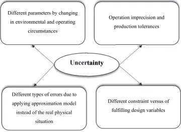
3.1.1. Different sources of uncertainty

Beyer and Sendhoff (2007) described four different types of uncertainties which a process might be collided by them as shown in Fig. 3. Another similar classification has been presented by Yjin and Branke (2005) which divided uncertainties into four categories, included noise in fitness functions, search for robust solutions, approximation error in the fitness function, and fitness functions changing over time. Also, another classification was proposed by Ho (1989) for production processes that divided uncertainty into two groups. First, an environmental uncertainty which includes uncertainties related to the process of production such as demand or supply uncertainty. Second, system uncertainty beyond uncertainties within the production process such as operation yield uncertainty, production lead time uncertainty, quality uncertainty, failure of the production system and changes to product structure (Mula et al., 2006).

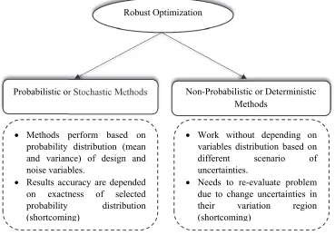
3.1.2. Classification of robust optimization models

Robust design with uncertainties has been distinguished a robustness design for constraints as well as objectives. There are various number of methods associated with robust design methodology in literature with different types of classification. One of the common classification is depicted in Fig. 4. As can be

Uncertainty

Operation imprecision and production tolerances Different parameters by changing

in environmental and operating circumstances

Different types of errors due to applying approximation model

instead of the real physical situation

Different constraint versus of fulfilling design variables

(6)

seen from this figure, robust optimization methods can be divided into two types of probabilistic and non-probabilistic approaches (Cao et al., 2015). In probabilistic or stochastic robust optimization methods, the designer performs the problem by employing the probability distribution of variables, particularly the mean and variation of uncertain or noise variables. It is clear that accuracy of obtained optimization results strongly depends on the accuracy of assumed probability distribution, in (Ardakani et al., 2009; Khan et al., 2015; Nha et al., 2013; Park & Leeds, 2015; Simpson et al., 2001) some applications of these types of robust optimization methods have been illustrated. Sometimes, the probability distribution of variables might be unknown or often difficult to obtain. Moreover, non-probabilistic or deterministic (distribution-free) methods could be used without depending on the size of variable variation region. This types of methods attempt to find robustness and optimum solution by recording different uncertainty sets in objective and constraint space. The main gap for these methods are that when uncertainties change in their variation region and previous results miss their validation, so it needs to designer evaluate problem again (Cao et al., 2015). To be more familiar with these types of methods see (Ben-Tal et al., 2009; Bertsimas et al., 2011; Ehrgott et al., 2014; Ide & Schobel, 2016; Salomon et al., 2014).

Among the study in literature, other classification of robust optimization problem could be defined when they are divided into two categories (Park & Lee, 2006). The first robust design optimization is based on Taguchi’s approach (Park & Lee, 2006; Park & Antony, 2008; Phadke, 1989) and the second robust optimization is based on uncertainty scenario sets (different combination of uncertainties) (Ben-Tal et al., 2009; Bertsimas et al., 2011; Gabrel et al., 2014). In this context, we concentrate more in Taguchi philosophy for the uncertain and noisy condition of the problem in the real world. Recent comprehensive overview of historical and technical aspects of robust optimization methods can be found in (Bertsimas et al., 2011; Beyer & Sendhoff, 2007; Dellino et al., 2015; Gabrel et al., 2014; Geletu & Li, 2014; Wang & Shan, 2011).

3.1.3 Robust Design Optimization Based on Taguchi’s Approach

The robust design methodology was introduced by Dr. Genichi Taguchi after the end of the Second World War and this method has developed over the last five decades. Quality control and experimental

Probabilistic or Stochastic Methods

Robust Optimization

Non-Probabilistic or Deterministic Methods

 Methods perform based on probability distribution (mean and variance) of design and noise variables.

 Results accuracy are depended on exactness of selected probability distribution (shortcoming)

 Work without depending on variables distribution based on different scenario of uncertainties.

 Needs to re-evaluate problem due to change uncertainties in their variation region (shortcoming)

(7)

design had strongly affected by Taguchi as a Japanese engineer in the 1980s and 1990s. Taguchi proposed that the term of quality should not be supposed just as a product being inside of specifications, but in addition to attending the variation from the target point (Shahin, 2006).

Phadke (1989) defined robust design as an “engineering methodology for improving productivity during research and development so that high-quality products can be produced quickly and at low cost”. The idea behind the robust design is to increase the quality of a process by decreasing the effects of variation without eliminating the causes since they are too difficult or too expensive to control. Park (1996) classified the major sources of variation into six categories included man, machine, method, material, measurement, and environment. The method of robust design is being into types of an off-line quality control method that design process before proceeding stage to improve productability and flexibility by creating process insensitive against environmental changeability and component variations. Totally, designing process that has a minimum sensitivity to variations in uncontrollable factors is the end result of robust design. The foundation of robust design has been structured by Taguchi on parameter design in a narrow sense. The concept of robust design has many aspects, where three aspects among them are more outstanding (Park & Antony, 2008):

1- Investigating a set of conditions for design variables which are insensitive (robust) against noise factor variation.

2- Finding at least variation in a performance around target point.

3- Achieving the minimum number of experiments by employing orthogonal arrays.

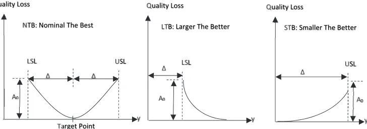
Robust design based on Taguchi approach has employed some statistically and analytically tools such as orthogonal arrays and Signal to Noise (SN) ratios. Furthermore, many designed experiments for determining the adequate combination of factor levels which are used in each run of experiments and for analyzing data with their interaction have been applied a fractional factorial matrix that called orthogonal arrays. The ratio between the power of the signal and the power of noise is called the signal to noise ratio ( ⁄ ). The larger numerical value of SN ratio is more desirable for process. There are three types of SN ratios which are available in robust design method depending on the type of quality characteristic, the Larger The Better (LTB), the Smaller the Better (STB), Nominal The Best (NTB). Both concepts of signal to noise ratio and orthogonal arrays have been described by most studies after first introducing by Taguchi in 1980s, so for more information see (Park, 1996; Park & Antony, 2008; Phadke, 1989).

Δ

LSL

USL

Quality Loss

y Target Point

0

A

NTB: Nominal The Best

Δ LSL

Quality Loss

y

0

A

LTB: Larger The Better

Δ

USL Quality Loss

y

0

A

STB: Smaller The Better

(8)

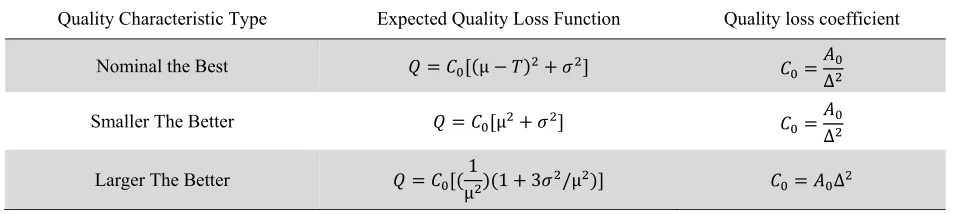
Table 2

Taguchi’s approach on quality loss function

Quality Characteristic Type Expected Quality Loss Function Quality loss coefficient

Nominal the Best μ

∆

Smaller The Better μ

∆

Larger The Better 1

μ 1 3 /μ ∆

Taguchi represented the concept of quality loss as an average amount of total loss that compels to society because of deviance from the ideal point and be variance in responses. Moreover, this function for each type of quality characteristics tries to create a trade-off between mean and variance. Fig. 5 depicts the expected loss function based on the well-known classification of quality characteristics into three different types of NTB, STB, and LTB. In addition, the expected quality loss function based on Taguchi’s approach for all three types of quality characteristics are represented in Table 2. Where in illustrated equations in Table 2, shows the expected quality loss and µ, σ2_{, T, and} _{respectively are quality} characteristic mean, variance, target and loss coefficient. The quality loss coefficient for each type of quality characteristic can be computed based on information about the losses in monetary terms when process specification is outside of the customer tolerance limits which is extracted from customer’s point of view as shown in Fig. 5. In addition, is introduced as a cost of repair or replacement when the quality characteristics performance has the distance of ∆ from target point (Phadke, 1989). Recently, the concept of quality loss function has been extended by some studies such as Sharma and Cudney (2011) and Sharma et al. (2007). As can be seen from the Table 2, the LTB case has more complexity than other two cases. The same formula for all three types of quality characteristics with more simplicity in relevant formulation has been proposed (Sharma et al., 2007). Their proposed formula is based on the lack of accessing target to infinity for LTB case, because it is unachievable. The proposed formulation could be replaced by all three types of expected quality loss mentioned in below:

1 , (2)

while in Eq. (2), is equal to when 0 and is a large number. The amount of could be defined by decision maker and is a target point for quality characteristic. For different values of the expected loss represents different expected losses for each type of NTB, LTB, or STB. This value shows the shifting of to right or left side of target point and can be chosen zero for STB type, a large number more than one is considered for LTB type and also 1 for NTB. But, it is strongly recommended that the target point and specially it does not need to be a large number or infinity for LTB cases, but it just needs to be significantly greater than one. It has recommended by Sharma et al. (2007) and Sharma and Cudney (2011) that in the case of LTB the magnitude of needs to significantly greater than one but not necessarily a large number or infinity, and they suggested 2 as an appropriate number to be employed in practice.

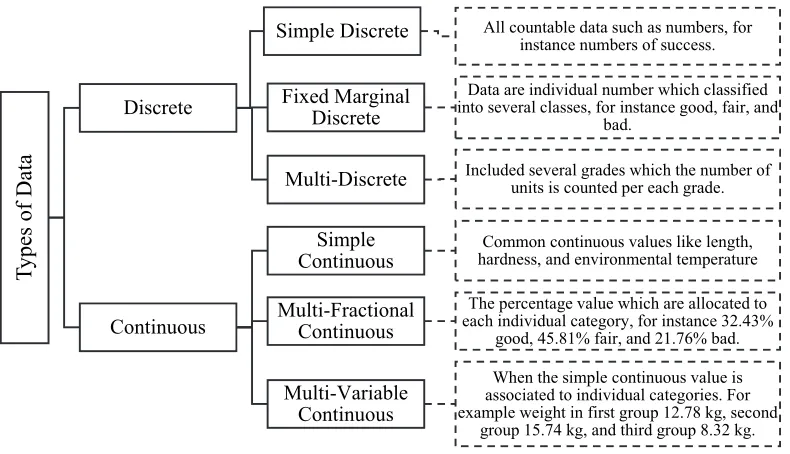
3.1.4. Classification of Factors and Data Types

(9)

Data in the experimental environment are usually divided into two different types of discrete and continuous. Taguchi has divided each of both types into three classes, as illustrated in Fig. 7 (Park 1996; Park & Antony, 2008).

Fig. 6. Different types of factors which influence process in practice

Types of Factor

Fixed Factors

Control (design)

Factors

Some design variables which during robust design process and its relevant experiment try to investigate the

best level of them.

Indicative Factors

Some factors which technically are the same with control factors, but the ‘best’ level for them is meaningless, for instance the locating in different

position such as being right, left, and straight..

Signal (target-control) Factors

The types of factors which just effect on mean and not make variability in responses (quality characteristic).

Random Factors

Block (group) Factors

Factors which classified in different levels, but these levels are not technically significant, differences depending on days, geographical location, or operators

are some instances of block factors.

Supplementary Factors

Factors which have been used as independent variables in the covariance analysis. These factors included supplementary experimental values which extracted

from state of experimental condition.

Noise (error) Factors

Uncontrollable factors that influence over responses in practice, and they are in three types included inner, outer

and between product noise factors.

Fig. 7. Types of data based on Taguchi approach

Types of Data

Discrete

Simple Discrete All countable data such as numbers, for instance numbers of success.

Fixed Marginal Discrete

Data are individual number which classified into several classes, for instance good, fair, and

bad.

Multi-Discrete Included several grades which the number of _{units is counted per each grade.}

Continuous

Simple

Continuous hardness, and environmental temperatureCommon continuous values like length,

Multi-Fractional Continuous

The percentage value which are allocated to each individual category, for instance 32.43%

good, 45.81% fair, and 21.76% bad.

Multi-Variable Continuous

When the simple continuous value is associated to individual categories. For example weight in first group 12.78 kg, second

(10)

This classification plays an important role in deciding about a number of necessity replications for experiments and determines the best method for analyzing data. In practice, the most process has been interfaced by a different combination of factors and data types, so it is important to consider them in robust design problem and define the robust optimization model. The survey in the literature revealed most studies have neglected to attend this importance for proposing comprehensive robust optimization method which can cover variety combination of factors with different types of data.

3.1.5 Dual Response Surface Method

Some authors like Myers et al. (2016) and Lin and Tu (1995) proposed to make a model based on separate process components included the mean and the variance. This methodology is adopted the so-called dual response surface approach. This model has employed a response surface for the process mean and another response surface for the process variance separately. This kind of model has been employed a type of design of sample point with a combination of both control and noise factors which is named combined array design. By combining both types of factors in process included design and noise factors, we can approximate the , as a function of number of design factors and number of uncertainties set .If we consider as a vector, which includes both sets of design and noise factors

thenthe mean and variance of each response (quality characteristic) based on the second order term of Taylor series by expanding around could be computed separately as follows,

1

2 . ∆ (3)

. . ∆ (4)

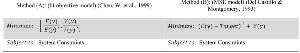
When the amount of ∆ depicts the covariance between ith and pth factors and is variance of ith factor when . Notably, there are different optimization approaches available on dual response methodology where some of them are referenced in (Ardakani & Noorossana, 2008; Beyer & Sendhoff, 2007; Nha et al., 2013; Yanikoglu et al., 2016), so here just for instance some common methods of them are mentioned in Table 3.

Table 3

Two methods of optimization based on dual response surface

Method (A): (bi-objective model) (Chen, W. et al., 1999) Method (B): (MSE model) (Del Castillo & _{Montgomery, 1993)}

: ∗, ∗ :

: System Constraints : System Constraints

3.1.6 Positive and Negative Points of View on Taguchi Approach

(11)

processes or product design in practice, and several appropriate studies have been reviewed the application of Taguchi methodology in real case studies, (e.g. Beyer & Sendhoff, 2007; Dellino et al., 2015; Gabrel et al., 2014; Geletu & Li, 2014; Park & Lee, 2006; Wang & Shan, 2011). In current reviewing of studies, the application of robust design methodology on optimizing the process in two types of production and project management were considered, whose results are described in section 4. On the other side about shortcomings of Taguchi’s idea in designing the process with a robust framework, some criticism have been extracted from different studies. Myers et al. (1990) presented an analytical study on Taguchi method. They mentioned five different criticisms of Taguchi’s approach in robust parameters design. The first one is the inefficiency of the signal to noise ratio. Second one is the shortage of ability in Taguchi design parameters to approach a flexible process modeling. The third one is the number of experiments in Taguchi robust design with their SN ratio that is not economical. Preoccupation with optimization is fourth, and fifth no formal allowance for sequential experimentation. The Taguchi approach with its crossed arrays and signal to noise ratios have emphasized the interaction between design variables with each other and have ignored the importance of interaction between design (control) and noise variables (Myers et al., 2016). In addition, some other drawbacks have been connected to traditional Taguchi’s approach. First, in designing variables with orthogonal arrays and signal to noise ratio, the process constraint are ignored for designing parameters, and secondly robust design with Taguchi approach just deals with a single quality characteristic as a response in each run of the method. So, it could not propose the best design by considering all responses at the same time. Thirdly Taguchi method just investigates the best levels of design variables in the discrete region and could not treat in whole design ranges (Dellino et al., 2015; Park & Lee, 2006).

3.1.7 Robust Optimization Based on Uncertainty Scenario Sets

While in Taguchi approach the procedure of designing variables with applying orthogonal array and signal to noise ratio has been done in discrete space, so it is impossible to investigate a wide range of design spaces. In practice, design in continuous space often is required as well. However, for the system different constraints could not be resolved by Taguchi parameter design, but in robust optimization method, the constraints under uncertainty can be easily covered (Park & Lee, 2006). Moreover, by facing real-world optimization problems, the standard techniques of mathematical programming can be used. A great number of studies have been performed where mathematical programming can contribute to robust optimization (Beyer & Sendhoff, 2007). Under the linear approach, we are interested in taking a suboptimal solution for the nominal values of the data in order to ensure feasibility of solution when it is near optimal. Bertsimas and Sim (2004) investigated the problem of solving linear robust optimization problems with uncertain data proposed in the early 1970s. A common structure of robust optimization under uncertainty (linear programming problem) is defined as follow:

: : , , , ∈ (5)

The data , , , varying around in a given uncertainty set and ∈ is the vector of decision variables, ∈ and ∈ form the objective, is an constraint matrix, and ∈ is the right hand side vector of constraint (Ben-Tal et al., 2009). In terms of stochastic optimization, we assume uncertain numerical data are random, and these random data in the simplest case follow certain probability distribution which is partially known in more setting of data. In this case the formulation is shown as below:

, : , , ~ & 1 , (6)

(12)

optimization problem. In literature different number of robust optimization methods have been defined in process engineering where recent and comprehensive technical reviews can be found (e.g. Bertsimas et al., 2011; Beyer & Sendhoff, 2007; Gabrel et al., 2014; Geletu & Li, 2014). Undoubtedly, Min-Max and two-stage approach have been widely used in region of robust optimization problems (Geletu & Li, 2014).

3.1.8 min max Approach

In the worst-case scenario of uncertainties, it is assumed that all variations of system performance may occur simultaneously in the worst possible combination of uncertainties. So, with respect to the min-max approach we try to minimize the maximum variability in the process performance due to the existence of uncertainty in their worst framework. The general formulation of min-max approach is shown below:

∈ ∈ ,

(7) subject to

∈ , 0 , 1,2, … ,

Since is design variables vector and is uncertainty set. In spite of some shortcoming such as tending to be overly conservative and may not cost-effective (Yu et al., 2015), this method provides a one-step formulation with optimal design and flexibility which has been employed in most problems as a common versatile approach (Ben-Tal et al., 2009; Geletu & Li, 2014). Furthermore, the optimization problem under uncertainty with min-max formulation expresses a problem of minimization of the worst case (maximum) influence of the uncertainties on the process performance.

3.1.9 Two-stage Approach

Because a solution of the single-stage robust optimization method must protect against any possible combination of uncertainty set, the single-stage tends to be excessively conservative and may not cost-effective. To address such a challenge, two-stage robust optimization method has been proposed to cover problem, where decisions to be divided into two stages included before and after uncertainty is revealed (Yu & Zeng, 2015). The first stage is that of variables that are chosen prior to the realization of the uncertain event. The second stage is the set of resource variables which illustrate the response to the first-stage decision and realized uncertainty. The objective is to minimize the cost of the first-first-stage decision and the expected value of the second-stage recourse function. The classic two-stage stochastic program with fixed resource is (Takriti & Ahmed, 2004):

, : , 0 . (8)

(13)

two-A. Parnianifard et al.

stage formulations has been employed in the real problem as well, for instances, (See Steimel & Engell, 2015; Zhang & Guan, 2014).

3.2. Robust design optimization hybrid metamodeling

Metamodeling is the analysis, construction, and development of the frames, rules, constraints, models and theories applicable and useful for modeling a predefined class of problems. Computation-intensive of design problems is becoming increasingly common in manufacturing industries. To address such a challenge, approximation or metamodeling techniques are often used. Metamodeling techniques have been developed from many different disciplines including statistics, mathematics, computer science, and various engineering disciplines (Wang & Shan, 2007). Furthermore, Metamodeling techniques have been used to avoid intensive computational and numerical simulation models, which might squander time and resource for estimating model's parameters. Metamodeling has utilized variety statistical and mathematical approach to interpreting parameters and their relationship in original models. If input or design variables and responses or outputs have a relationship as then a model of the model or meta-model which approximate the relationship is and where ɛ represents an error of approximation (Simpson et al., 2001). Some simulation optimization methods have been introduced by Anderson et al., (2015) and Carson & Maria (1997). Metamodeling methods have been

greatly applied in engineering design when the problem is computationally expensive and needs to be improved by more flexibility in the model (Jin, R. et al., 2003). There are different number of methods which have been introduced as meta-models to approximate the relationship between response and design variables of process, and they can be found in several comprehensive technical surveys in literature. In addition, Investigating in literature shows that two versatile methods, RSM and Kriging, have been applied more in different optimization problems in the real world (See Dellino et al., 2015; Jin et al., 2003; Simpson et al., 2001; Wang & Shan, 2007).

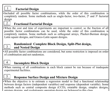
3.2.1 Classification of Experimental Design

The design of experiments (DOE) methodology plays an important role in the construction of a meta-model by proposing a limited number of experiments as much as possible (Kartal-Koç et al., 2012).

Factorial Design 1

•Included all possible factor combinations, while the order of this combination is completely random. Some methods such as single-factor, two-factor, 2k _{and 3}k_factorial design

Fractional Factorial Design 2

•When the cost and time of experiments are important to control, so the fraction of all possible factor combinations can be used, while the order of this combination is completely random. Some methods such as orthogonal arrays, Placket-Burman design, Latin square designs, and Graeco-Latin square designs.

Randomized Complete Block Design, Split-Plot design, and Nested Design

3

•All possible factor combinations are considered, but some restriction is imposed on order of combination and not randomize.

Incomplete Block Design 4

•When running of all combinations in each block cannot be run because of inadequate experimental facilities.

Response Surface Design and Mixture Design 5

•When the objective is to estimate a regression model to find a functional relationship between design factors (independent variables) and response (dependent variable). Some methods such as central composite design (CCD), rotatable design, simplex designs, mixture designs, and evolutionary operation design are belonged to this class.

(14)

The science of experimental design included some integrated techniques is used to increase the efficiency of obtained information and analyzing them. The basic principles of DOE includes factorial design and analysis of variance (ANOVA) was first introduced by Fisher in the 1920s in England and was presented in his book in 1935 as the first book on experimental design, (See Park & Antony, 2008). Shortly after, the concept of DOE was employed by a great numbers of engineers to improve different processes performance in the real world, and today there are a number of studies which have developed the traditional concept of DOE, see (Myers et al., 2016; Park, 1996; Park & Antony, 2008) and recent study (Kartal-Koç et al., 2012). There are various types of experimental designs which determine strategies to locate needs sample points in design region in such way to achieve at least variance. Park and Antony (2008) classified the experimental designs based on different factor combinations and the amount of randomization of experiments, which illustrates in Fig. 8.

3.2.2 Response Surface Design (RSM)

Because of the variance in the objective function, robust optimization has needed second-order derivatives against nonlinear programming. Though both nonlinear programmings with second-order derivatives could be used in problem (Park & Lee, 2006). Nowadays, the application of the Response Surface Methodology (RSM) is being significantly increased. The RSM has been used for approximation and more investigation robustness in robust design approach. The response surface methodology based on polynomial regression has been widely applied in engineering design. Different statistical and mathematical techniques have been used in RSM for developing, improving, and optimizing the process. The expression of the second-order response surface model is shown as below framework:

, 2 , (9)

where , and are unknown regression coefficients and the term is the usual random error (noise) component (Myers et al., 2016). The functional purposes of RSM which are found in literature can be mentioned as below:

1- Approximate the relationship between design (dependent) variables and single or multi-response (independent variables).

2- Investigating and determining the best operating condition for the process, by finding the best levels of design region which can satisfy operating limits.

3- Implementing robustness in quality characteristics of the process by finding robust designing in the process.

3.2.3 Kriging

Since Krige (1951) addressed the geostatistics, today Kriging models have been used as a widespread global approximation technique (Jurecka, 2007). Kriging is an interpolation method which could cover deterministic data, and it is highly flexible due to ability in employing a various range of correlation functions. The higher accuracy of Kriging models than the other alternatives such as response surface modeling are confirmed in the literature (Dellino et al., 2015; Simpson et al., 2001). In a Kriging model, a combination of a polynomial model and realization of a stationary point are assumed by the form of:

(10)

(15)

most time normally distributed Gaussian random process with zero mean, variance and non-zero covariance. The correlation function of is defined by:

, , , (11)

where is the process variance and , is the correlation function, and can be chosen from different functions proposed in the literature. Due to tuning the correlation function with sample data, the Kriging is extremely flexible to capture nonlinear treatment of model (Jin et al., 2003). Among literature, some studies have been found which sufficiently describe Kriging metamodel methodology, (Dellino, 2015; Jin et al., 2003; Jurecka, 2007; Simpson et al., 2001).

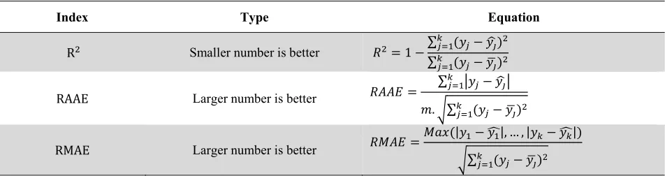
3.2.4 Evaluating Metamodels

There are number of indexes to evaluate metamodel accuracy, see (Cao et al., 2015; Dellino et al., 2009; Jin et al., 2003; Wang & Shan, 2007).

Table 4

Metamodels measurement metrics

Index

Type Equation

R Smaller number is better 1 ∑

∑

RAAE Larger number is better

∑

. ∑

RMAE Larger number is better

| |, … , | |

∑

Three common methods are , Relative Average Absolute Error (RAAE), and Relative Maximum Absolute Error (RMEA), which are defined in Table 4. In all equations of Table 4, is mean of observed values ( ) and is corresponding predicted values. Also, the large number of square and small number of RAAE and RMEA is depicted more accuracy in metamodel.

3.3. Multi-objective robust optimization

In practice, the designer often has to deal with problems that involve conflicting objectives and source of uncertainty. The prospering in methods of Multi-Objective Robust Optimization (MORO) could be divided into previous and recent studies. Previously, robust design approach has been combined with some different methods in multi-objective optimization such as the weighted sum method (Zadeh, 1963), goal programming (Charnes & Cooper, 1977), physical programming (Messac & Ismail-Yahaya, 2002), compromise programming (Chen et al., 1999), desirability function (Costa et al., 2011) and Lp metrics methods (Miettinen, 2012). Recently, some developed methods have been proposed as evolutionary algorithms such as simulated annealing (Suman & Kumar, 2006), particle swarm optimization (Parsopoulos & Vrahatis, 2002) and non-dominated sorting genetic algorithm (Deb et al., 2002), and Non-dominated Sorting Genetic Algorithm II (NSGA-II) (Martınez-Frutos & Marti-Montrull, 2012).

(16)

employed in the most multi-objective problem are the desirability function (Chen et al., 2011), an evolutionary algorithm (Deb, 2011), and different metrics methods (Hwang & Masud, 2012). The weighted Lp metric method could be applied in the robust multi-objective to find a Pareto optimal solution, (See Ardakani & Noorossana, 2008). The Lp metric is used to measure the distance between objectives (responses) of the process and the relevant target points. The overall function to integrate all responses with Lp metric method used Eq. (12):

(12)

Since is the ideal point for kth response and the quantity of shows the importance of kth response compared to others and can take a value between zero and one, so that ∑ 1 and assigned by the decision maker. The value of while 1 ∞ indicates the emphasizing on deviation of each function from the target point. As a general, the cases of 1,2, … , ∞ is more common to employ in computational models, (See Miettinen, 2012). Notable in above, all responses must have the same scales in the formulation. When responses do not have the same scale, each response could be scale less by applying Eq. (13):

(13)

Here is the worst value which can be allocated to kth response in design variables region of (Ardakani & Noorossana, 2008; Miettinen, 2012). In the aforementioned method, the correlation between responses (quality characteristics) is ignored, and independence between them is assumed. In practice the variance of each quality characteristic is not constant over the experimental space. Under such condition, the multi-response model must be able to consider the correlation among quality characteristic. A number of recent studies which have been attended variance-covariance framework of responses are Cheng et al. (2013), Rathod et al. (2013), Romano et al. (2004) and Salmasnia et al. (2013).

3.4. Dynamic Problems (Robust Optimization over Time)

In real-word problems, most optimization problems, often have faced to various changing in their environment. In an optimization problem, each change in condition can involve variation in the problem components such as objective functions, design variables, environmental or noise factors as well as constraints. The number of problem components (objectives, design variables, and constraints) might vary over time during the optimization. For instance, in the social problem, the population size is such a dynamic factor which change from time to time (Jin et al., 2013). To address such a challenge, the Dynamic Optimization Problems (DOPs)(Fu et al., 2015) have been employed to propose robust optimal solution over time. So the existing static models have to be revised to dynamic approach in uncertainty environment as Robust Optimization Over Time (ROOT) (Beyer & Sendhoff, 2007; Jin et al., 2013). However, few studies have been concerned with optimizing the robust design optimization over time involving static and dynamic components, see (Fu et al., 2015; Jin & Branke, 2005; Wu & Yeh, 2009; Wu, 2015).

3.5. Multi-Process System

(17)

continue in the direction of distinct system objectives, as shown in Fig. 9. The optimization model must be able to handle a trade-off between the best performance from all processes and system cost. Different types of uncertainty and noise factors, and also changeability in goals over time can influence on each process separately in a multi-process environment. Moreover, optimization methods need to be developed for optimizing all interacted process in a multi-process situation as well as optimizing one process at the same time (Bertsekas, 1998). So, among reviewing articles, extending proposed robust optimization methods into the multi-process environment was considered, which the results are shown in section 4.

3.6. Production and Project Management under Uncertainty

In practice, as well as various problems in engineering processes and systems, management methodologies could be affected by uncertain parameters which create deviance between the result of optimization model with the target. Proposing a robustness designs for these types of problem are purposes of most studies which have been employed robust design optimization approach. Developing traditional methods under uncertain and noisy conditions into two main methodologies of management science such as production management and project management have been considered in studies. Production planning, job shop, and flow shop scheduling in production management and project scheduling with a trade-off between time, cost and quality are some important problems in both methodologies of production and project management. Robust optimization methods attempt to model production planning problem in such a way to minimize cost, wastage, and effect of uncertainties or risk and also maximize the total expected profit (Ait-Alla et al., 2014). Among literature, in production management methodology, two main problems included first robust production planning, (See Ait-Alla et al., 2014; Asih & Chong, 2015; Gyulai et al., 2015; Khademi Zare et al., 2006; Mirzapour Al-e-Hashem et al., 2011) and comprehensive review study (Mula et al., 2006) and second robust supply chain (for example see (An & Ouyang, 2016; Hasani & Khosrojerdi, 2016; Pishvaee & Torabi, 2010; Pishvaee et al., 2011, 2012) under uncertain condition which has been more considered than other relevant parts. In real word delivering projects on time within certain budget by covering all needed project specifications, still seems extremely difficult (Demeulemeester & Herroelen, 2011). The majority of previous relevant studies just have concentrated to schedule project in the certain and deterministic

environments, in spite of the existence of various types of uncertainties in project conditions, such as uncertainty in activity duration, predecessors, and resources (human, machine, budget). Project are often faced with various types of uncertainties that have a negative influence on project components such as activity duration and costs. So it is crucial to modify effective methods to a robust schedule of the project which is less sensitive to the variability of uncontrollable factors (Hazir et al., 2010). Herroelen and Leus (2004) and (2005) in two different comprehensive review papers have tried to investigate the methods of reactive and proactive scheduling project under uncertain conditions. In addition, recent survey on scheduling problems based on time and cost can be found in (Allahverdi, 2015).

Fig. 9. A general overview of multi-process system

Output of System Process

1

Process 2

Process 3

Process 4

Process 5

Process 6

Process N-3

Process N-2

Process N-1

Process N

(18)

4. Discussion and results

All selected articles were systematically analyzed included in-depth review, evaluate and interpret of each article methodologies of research. Relevant information was extracted to a predefined database.

4.1. Methodologies

Throughout the literature review, several important methods were investigated in selected articles, which are separately classified as following. Note that in continuing definition of each class, the term of “problem” is a contraction of robust design optimization for the process by considering uncertainty or noise factors.

M.1: Articles which have employed the classic concepts of robust design such as Taguchi parameters design with orthogonal arrays, signal to noise ratio or quality loss function approach to improving product and process.

M.2: The method of mathematical programming in both approaches of robust design optimization included Taguchi approach and scenario sets have been used by articles in this class.

M.3: Multi-objective problems and relevant methods have been attended by this class’s articles for problems under uncertainty.

M.4: Metamodels methodology were contributed by robust design optimization for the designing process under uncertainty with minimum computational complexity.

M.5: In problem environment, the fuzzy approach has been considered in facing by uncertainties. M.6: The distinct strategy in conflicting with uncertainty or noise factors in problem have been proposed. M.7: The proposed methods by articles in this class are able to extend and generalized in some other process optimization problem, and not limited to specific condition or location of the problem.

M.8: The computational complexity and time consuming to solve the relevant problem have been considered.

M.9: The process cost next to the process performance has been kept as problem objectives. It means proposed optimization method has been able to handle a trade-off between cost and performance. M.10: Multi-process environment as a system (Fig. 9) which consists of several interlinked processes have been considered in the problem by selected articles in this class. Notably, some studies in this class just consider the concept of network in their studies where their approaches have been able to accommodate into multi-process systems and not attended the concept of multi-process directly. The trade-off between the best performance of all processes and the total cost is the main purpose of optimization in the multi-process system.

M.11: The uncertainty in physical constraints have been considered as well as the objectives to optimize process and find global robustness solution.

M.12: Articles in this class have attended dynamic optimization method over time for their problem. M.13: Different combinations of data included discrete and continuous data (Fig. 7) have been handled by proposed method.

M.14: The proposed method have been able to consider different probability distributions in the process for design or noise variables, in stochastic programming, or method is distribution free.

4.2. Analysis and interpreting

(19)

4.3. Discussion

To analyze the results in Table 6, we consider the proportion of articles in both groups of objective and methodology. Fig. 10 illustrates the proportion of articles (total 150 articles) in each class of methodology. Consequently, as can be seen from the figure and also by a systematic review of selected articles, several important points are concluded as the findings of this study. In addition to the selected articles, a brief glance of almost other relevant literature could demonstrate the mentioned points. 1- To the best of our knowledge, there are not adequate cases in literature that compare different methods

of metamodeling faced with robust optimization models for the real problem in practice with uncertain and noise parameters. The various methods of metamodeling have never compared to each other about where metamodel is definitely superior to others according to real circumstances of the problem (Beyer & Sendhoff, 2007; Jin, et al., 2001; Jurecka, 2007; Wang & Shan, 2007). In optimizing the process, by attending uncertainty, multi-objectives, and dynamic parameters over time the computational complexity increase more and more, since metamodels could reduce computational time and cost consuming, see (Ateme-Nguema et al., 2012).

2- In multi-objective optimization problems, metamodels could be used to reach an approximation of an overall objective function, but their relevant application is not straightforward as well as classical, evolutionary, or meta-heuristic algorithms (Dellino et al., 2009).

3- The trade-off between time, cost and quality has not been extensively done in the literature yet for problems under uncertainty (Salmasnia et al., 2012). This subject is vital for appropriate scheduling of projects in practice.

4- In the case of dynamic programming over time, few models could be found were mainly theoretical particularly in problems under different types of uncertainty et al., 2009; Wu, 2015). For instance in robust design problems, most models did not pay much attention to the time value of money for quality loss and product degradation over time (Peng et al., 2008).

5- To the best of our knowledge, there are no considerable works on proposing methods which cover different types of data mentioned in Fig. 7 (discrete and continues data for design variables and also noise factor), in spite of importance function of these types of data with different combination in practice (Bertsimas & Sim, 2004).

6- In practice, most systems consist of several interacted processes by intensive linking to each other. Optimizing a multi-process environment under noise and uncertain uncontrollable parameters have not been considered as well as a single process problem. Most of the times, the results which are obtained separately for each single process, could not be expanded for the whole system, while it needs trade-off between results.

(20)

Table 5

Findings of review articles based on objective and methodology

No

Ref. Methodology

M.1 M.2 M.3 M.4 M.5 M.6 M.7 M.8 M.9 M.10 M.11 M.12 M.13 M.14

1 (Huang et al., 2016) √

2 (Kokkinos & Papadopoulos, 2016) √ √ √ √ √ √ √ √

3 (Wu et al., 2016) √ √ √

4 (Kuhn et al., 2016) √ √ √ √

5 (Salmasnia et al., 2016) √ √ √ √ √

6 (Ide & Schobel, 2016) √ √ √ √ √

7 (Zhang & Lu, 2016) √ √ √ √

8 (Grossmann et al., 2016) √ √ √ √

9 (Wang et al., 2016) √ √ √ √ √ √

10 (Kolluri et al., 2016) √ √ √ √ √ √ √

11 (Tsai & Liukkonen, 2016) √ √ √ √ √ √

12 (Zhang et al., 2016) √ √ √ √ √

13 (Talaei et al., 2016) √ √ √ √ √ √

14

(Palacios et al., 2016) √ √ √ √ √ √ √

15 (Ghodratnama et al., 2015) √ √ √ √ √ √

16 (Pishvaee & Fazli Khalaf, 2016) √ √ √ √ √ √

17 (Wu et al., 2016) √ √ √ √ √

18 (Zhang et al., 2016) √ √ √ √ √ √

19 (Namazian & Yakhchali, √ √ √ √ √ √ √

20 (Wu et al., 2016) √ √ √ √ √

21 (Tabrizi & Ghaderi, 2016) √ √ √ √ √ √

22 (Aalaei & Davoudpour, 2017) √ √ √ √

23 (An & Ouyang, 2016) √ √ √ √

24 (An et al., 2016) √ √

25 (Cai et al., 2016) √ √ √ √ √ √ √

26 (Gang et al., 2015) √ √ √ √

27 (Lersteau et al., 2016) √ √ √ √

28 (Mirmajlesi & Shafaei, 2016) √ √ √ √

29 (Modarres & Izadpanahi, √ √ √ √ √

30 (Ling et al., 2017) √ √ √ √

31 (Peri, 2016) √ √ √ √ √ √

32 (Gul & Zoubir, 2017) √ √ √

33 (Goerigk & Schöbel, 2015) √ √ √ √ √

34

(Gorissen, 2015) √ √ √ √ √ √

35 (Liu et al., 2015) √ √ √ √

36 (Sun et al., 2015) √ √ √

37 (Fu et al., 2015) √ √ √ √

38

(Wu , 2015) √ √ √ √ √

39 (Khan et al., 2015) √ √ √

40

(Park, 2016) √ √ √

41 (Goberna et al., 2015) √ √ √ √

42

(Wang, 2015) √ √ √

43 (Wang & Pedrycz, 2015) √ √ √ √ √

44 (Yu & Zeng, 2015) √ √ √

45 (Asafuddoula et al., 2015) √ √ √ √ √ √

46 (Dellino et al., 2015) √ √ √ √ √ √ √ √ √

47 (Auzins et al., 2015) √ √ √ √ √ √

48 (Cao et al., 2015) √ √ √ √ √ √

49 (Ng et al., 2015) √ √ √ √ √ √ √

50

(21)

Table 5

Findings of review articles based on objective and methodology (Continued)

No

M.1

M.2 M.3 M.4 M.5 M.6 M.7 M.8 M.9 M.10 M.11 M.12 M.13 M.14

51 (Bossaghzadeh et al., 2015) √ √ √ √ √

52 (Zhang & Qiao, 2015) √ √ √ √ √ √

53 (Mavrotas et al., 2015) √ √ √ √ √ √

54 (Fu et al., 2015) √ √ √ √ √

55 (Sahali et al., 2015) √ √ √ √ √ √

56 (Gyulai et al., 2015) √ √ √ √ √ √

57 (Gabrel et al., 2014) √

58 (Ehrgott et al., 2014) √ √ √ √ √ √ √

59 (Bandi & Bertsimas, 2014) √ √ √ √ √

60 (Celano et al., 2014) √

61 (Geletu & Li, 2014) √ √ √ √ √ √ √

62 (Iancu & Trichakis, 2014) √ √ √ √ √

63 (Margellos et al., 2014) √ √ √ √ √ √

64 (Salomon et al., 2014) √ √ √ √ √ √ √

65 (Ur Rehman et al., 2014) √ √ √ √ √

66 (Can et al., 2014) √ √ √ √

67 (Oros et al., 2014) √ √ √ √ √

68 (Chevalier et al., 2014) √

69 (Jin et al., 2014) √ √ √ √ √ √

70 (Hao et al., 2014) √ √ √ √ √

71 (Wu et al., 2014) √ √ √ √ √ √ √

72 (Khaledi et al., 2014) √ √ √ √

73 (Dellino et al., 2012) √ √ √ √ √ √ √ √

74 (Ait-Alla et al., 2014) √ √ √ √ √

75 (Persson & Ölvander, 2013) √ √ √ √ √

76 (Artigues et al., 2013) √ √ √ √ √

77 (Gulpinar & Pachamanova, √ √ √ √

78 (Zhang, Siliang et al., 2013) √ √ √ √

79 (Nha et al., 2013) √ √ √ √ √ √

80 (Zhu et al., 2013) √ √ √ √ √ √ √

81 (Salmasnia et al., 2013) √ √ √

82 (Rathod et al., 2013) √ √ √ √ √ √

83 (Cheng et al., 2013) √ √ √ √ √

84 (Dalton et al., 2013) √ √ √ √ √ √

85 (Jin et al., 2013) √ √ √ √ √ √ √

86 (Kartal-Koç et al., 2012) √ √ √

87 (Martınez-Frutos & Marti-Montrull, 2012)

√ √ √ √ √ √ √

88 (Pishvaee & Razmi, 2012) √ √ √ √ √

89 (Lopez Martin et al., 2012) √ √

90 (Salmasnia, Ali et al., 2012) √ √ √ √ √

91 (Fu et al., 2012) √ √ √ √ √

92 (Bertsimas et al., 2011) √ √ √ √ √

93 (Klimek & Lebkowski, 2011) √ √ √

94 (Lambrechts et al., 2011) √ √ √

95 (Sharma & Cudney, 2011) √ √ √

96 (Erdbrügge et al., 2011) √ √ √ √ √

97 (Mirzapour Al-e-Hashem et √ √ √ √ √ √

98 (Miranda & Castillo, 2011) √ √

99 (He et al., 2010) √ √ √ √

(22)

Table 5

Findings of review articles based on objective and methodology (Continued)

No

M.1

M.2 M.3 M.4 M.5 M.6 M.7 M.8 M.9 M.10 M.11 M.12 M.13 M.14

101 (Datta & Mahapatra, 2010) √ √ √ √ √

102 (Dellino et al., 2010b) √ √ √ √ √ √ √

103 (Dellino et al., 2010a) √ √ √ √ √ √ √

104 (Sun, Wei et al., 2010) √ √ √ √ √ √

105 (Yu et al., 2010) √ √ √ √ √ √

106 (Hazir et al., 2010) √ √ √ √ √ √

107 (Ardakani et al., 2009) √ √ √ √ √

108 (Adida & Joshi, 2009) √ √ √ √

109 (Dellino et al., 2009) √ √ √ √ √ √ √ √

110 (Dellino et al., 2009) √ √ √ √

111 (Wu & Yeh, 2009) √ √ √ √

112 (Hasuike & Ishii, 2009) √ √ √ √ √ √

113 (Hahn, 2008) √ √ √

114 (Peng et al., 2008) √ √ √ √ √ √ √

115 (Ardakani & Noorossana, √ √ √ √ √

116 (Stinstra & den Hertog, 2008) √ √ √ √ √

117 (Beyer & Sendhoff, 2007) √ √ √ √ √ √ √ √ √ √ √

118 (Wang & Shan, 2007) √ √ √

119 (Cohen et al., 2007) √ √ √ √ √ √

120 (Yamashita et al., 2007) √ √ √ √

121 (Janak et al., 2007) √ √ √ √ √ √

122 (Sharma et al., 2007) √ √ √

123 (Singh et al., 2007) √ √ √

124

(Popescu, 2007) √ √ √ √ √

125 (Park & Lee, 2006) √ √ √ √ √

126

(Shahin, 2006) √

127 (Khademi Zare et al., 2006) √ √ √ √ √ √

128 (Mula et al., 2006) √ √ √ √ √ √ √

129 (Herroelen & Leus, 2005) √ √ √ √ √ √

130 (Ko et al., 2005) √ √ √

131 (Jin & Branke, 2005) √ √ √ √ √

132

(Chen, 2004) √ √ √

133 (Herroelen & Leus, 2004) √ √ √ √ √

134 (Antoniol et al., 2004) √ √ √

135 (Bertsimas & Sim, 2004) √ √ √ √ √ √

136 (Romano et al., 2004) √ √ √ √ √

137 (Lehman et al., 2004) √ √ √ √ √

138 (Jin et al., 2003) √ √ √ √ √ √

139 (Messac & Ismail-Yahaya, √ √ √ √

140 (Sandgren & Cameron, 2002) √ √ √ √

141 (Simpson et al., 2001) √ √ √ √

142 (Jin et al., 2001) √ √ √

143 (Chou & Chang, 2001) √ √ √ √

144 (Lee & Tang, 2000) √ √ √

145 (Chen et al., 1999) √ √ √ √ √

146 (Mavris et al., 1999) √ √ √ √ √ √ √ √

147 (Ahmed & Sahinidis, 1998) √ √ √ √ √ √ √

148 (Su & Renaud, 1997) √ √ √

149 (Myers et al., 1997) √ √ √ √ √ √

(23)

5. Conclusion

Accurate optimization of the process has been the main goal of many methods, since, most processes become to be more complex in practice. An unknown environment with variety types of uncertainties, intensive changes, uncontrollable factors, dynamic parameters over time, conflicting number of responses (multi-response), different types of data and so on, are some important circumstances which increase computational complexity in the problem. Therefore, some methods have been attracting intensive attention for tackling these conditions. Moreover, this study was aimed to systematically review some available literature on studies for such problems. The findings have revealed that there is still a gap between theory and practice in optimization, being evident in the fact that optimization methods could not still be used for many real-world problems. It is because most optimization methods have collided by some constraints and drawbacks such as inattention to uncertainties, the effect of noise factors, multi-response condition, dynamic parameters and also intensive computation attempts. Furthermore, proposing comprehensive methods which can handle aforementioned circumstances, can be suggested for further research.

References

Aalaei, A., & Davoudpour, H. (2017). A robust optimization model for cellular manufacturing system into supply chain management. International Journal of Production Economics, 183, 667–679. Adida, E., & Joshi, P. (2009). A robust optimisation approach to project scheduling and resource

allocation. International Journal of Services Operations and Informatics, 4(2), 169–193.

Ahmed, S., & Sahinidis, N. V. (1998). Robust Process Planning under Uncertainty. Industrial &

Engineering Chemistry Research, 37(5), 1883–1892.

Ait-Alla, A., Teucke, M., Lutjen, M., Beheshti-Kashi, S., & Karimi, H. R. (2014). Robust production planning in fashion apparel industry under demand uncertainty via conditional value at risk.

Mathematical Problems in Engineering, 2014.

Allahverdi, A. (2015). The third comprehensive survey on scheduling problems with setup times/costs.

European Journal of Operational Research, 246(2), 345–378.

An, K., & Ouyang, Y. (2016). Robust grain supply chain design considering post-harvest loss and harvest timing equilibrium. Transportation Research Part E: Logistics and Transportation Review, 88, 110– 128.

An, Q., Bai, G., Yang, Y., Wang, C., Huang, Q., Liu, C., … Xiang, B. (2016). Preparation optimization

Fig. 10. The proportion of articles in each class of methodology

15.13%

73.03%

28.29% 23.03%

13.16% 76.97%

62.50% 51.32%

50.00%

5.26% 65.13%

8.55% 3.29%

12.50%

0% 10% 20% 30% 40% 50% 60% 70% 80% 90%