www.ocean-sci.net/12/369/2016/ doi:10.5194/os-12-369-2016
© Author(s) 2016. CC Attribution 3.0 License.
Indian Ocean Dipole modulated wave climate
of eastern Arabian Sea
T. R. Anoop1, V. Sanil Kumar1, P. R. Shanas1,2, J. Glejin1, and M. M. Amrutha1
1Ocean Engineering Division, CSIR-National Institute of Oceanography (Council of Scientific & Industrial Research),
Dona Paula, Goa 403 004, India
2Marine physics department, King Abdulaziz University, Jeddah, Saudi Arabia
Correspondence to: V. Sanil Kumar ([email protected])
Received: 8 September 2015 – Published in Ocean Sci. Discuss.: 27 October 2015 Revised: 6 February 2016 – Accepted: 16 February 2016 – Published: 7 March 2016
Abstract. Intrinsic modes of variability have a significant role in driving the climatic oscillations in the oceanic pro-cesses. In this paper, we investigate the influence of an inter-annual mode of variability, the Indian Ocean Dipole (IOD), on the wave climate of the eastern Arabian Sea (AS). Using measured, modeled and reanalysis wave data and reanalysis wind data, we show that the IOD plays a major role in the variability of wave climate of the study region. Due to the IOD-induced changes in equatorial sea surface temperature and sea level pressure, the winds from the northern AS gets modified and cause inter-annual variability in the wave cli-mate over the eastern AS. The changes in wind field over the AS due to the IOD influence the generation or dissipation of the wave field and hence cause a decrease in northwest short-period waves during positive IOD and an increase dur-ing negative IOD.
1 Introduction
The northern Indian Ocean (IO) is a unique ocean as com-pared to northern Atlantic and Pacific oceans. Because of the land-locked northern boundary, the wind pattern in this re-gion shows semiannual reversal and causes boreal summer (June–September) and winter (December–February) mon-soons. Strong westerly wind in the equatorial IO is limited to short transition periods between the monsoons – both south-west (SW) and northeast (NE). The equatorial zonal wind reaches a maximum in April–May and in October–November (Hastenrath and Polzin, 2004). The wind in the eastern
Long-period southern hemispheric swells are present in the east-ern AS except during the SW monsoon season (Glejin et al., 2013a).
The monsoon wind patterns in the northern IO affect the spatial distribution of sea surface temperature (SST) in the tropical IO. The SST distribution differs from that observed in the Pacific and Atlantic which are warmer in the west (Vinayachandran et al., 2009). In the IO, warm water is on the eastern side and cold water is on the western side (Vinay-achandran et al., 2009). This SST difference varies during the coupled oceanic and atmospheric phenomena in the equato-rial IO known as the Indian Ocean dipole (IOD) (Saji et al., 1999). Positive IOD (PIOD) is associated with decreases (in-creases) of SST and increases (de(in-creases) of sea level pres-sure (SLP) over the eastern (western) tropical IO. The nega-tive phase of IOD is intensification of the normal condition (Vinayachandran et al., 2009). In the equatorial IO, the IOD appears as a dominant contributor of SST variability during the boreal fall season (October–December) (Saji and Yam-agatta, 2003). About 12% of the SST variability in the IO is associated with dipole mode events (Vinayachandran et al., 2009). There is a phase lag in the SST evolution be-tween the eastern and western tropical IO (Saji et al., 2003) and the regions of positive anomaly (during PIOD) vary with year (Vinayachandran et al., 2009). The Dipole Mode Index (DMI) is a quantitative representation of the strength of the IOD and is a measure of the anomalous zonal SST gradient across the equatorial IO. It is defined as the differ-ence between SST anomaly in a western (60–80◦E, 10◦S– 10◦N) and an eastern (90–110◦E, 10–0◦S) box. Seasonal phase locking is an important characteristic of the DMI time series. It is moderately correlated with the nino3 (ENSO) in-dex, but it is strongly correlated with equatorial winds over the IO (Saji et al., 1999). Monthly DMI are available on the website of the Japanese Agency of Marine–Earth Science and Technology (www.jamstec.go.jp).
The tropical IO displays strong inter-annual climate vari-ability associated with the El Niño–Southern Oscillation (ENSO) and the IOD (Murtugudde et al., 2000; Slingo and Annamalai, 2000). Baquero-Bernal et al. (2002) found that the IOD shows good correlation with the ENSO in the equa-torial Pacific Ocean. However, the correlation between the strength of ENSO and IOD is not linear (Shinoda and Han, 2005). IODs co-occurring with ENSO are forced by a zonal wind shift in the descending branch of Walker circulation in the eastern IO and the process that initiates IODs in the ab-sence of ENSO is not clear (Vinayachandran et al., 2009).
The impact of IOD on the wind pattern in the equato-rial IO is examined in the following studies. SST and SLP variation produced by the IOD cause easterly zonal wind anomaly especially in its zonal component in equatorial IO (Reverdin, 1985; Murtugudde et al., 2000; Saji et al., 1999; Webster et al., 1999; Sreenivas et al., 2012). The IOD-forced wind anomalies are maximum in the central equatorial IO (Sreenivas et al., 2012) – significant anomalies appear around
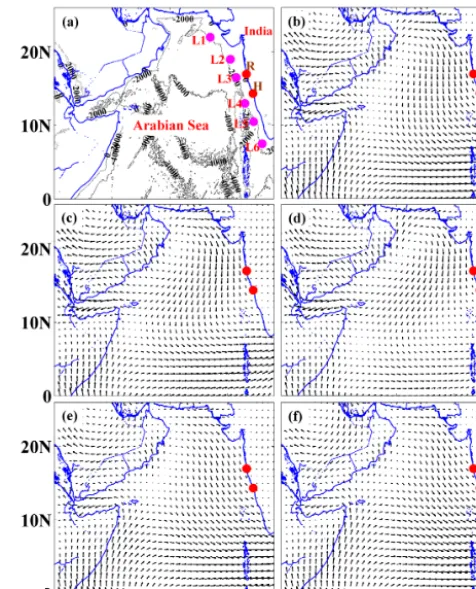
Figure 1. (a) The six locations considered to study the role of DMI on the wave climate are L1 to L6. The wave-measuring locations (Ratnagiri and Honnavar) in central eastern AS are shown as red dots. (b) Composite climatology of wind pattern during October in the AS and part of the equatorial Indian Ocean from 1958 to 2014. Averaged wind pattern during (c) pure positive IOD, (d) combined positive IOD, (e) pure negative IOD and (f) combined negative IOD from 1958 to 2014.
June, intensify in the following months and peak in October. The anomalous easterlies weaken the eastward Wyrtki jets (Wyrtki, 1971) in the equatorial IO (Reverdin, 1985). The wind anomaly produced during IOD has longer duration, but ENSO has shorter duration (Rao et al., 2002).
mod-els are described in Sect. 2. Section 3 describes results and discussion, and the main findings are summarized in Sect. 4.
2 Data and methods
The major challenge for wave climate study in the eastern AS is the scarcity of long-term observational data. In this study we use the available measured data of the Datawell di-rectional waverider buoy off Ratnagiri (available from 2010 to 2014) and off Honnavar (available from 2008 to 2014) off the central west coast of India. Among these, Ratnagiri is the northern and Honnavar is the southern location and these locations are spaced∼350 km apart. The details of the data analysis are similar to those presented in Sanil Kumar et al. (2014). The spectral climatology of the study area is presented by Sanil Kumar and Anjali Nair (2015).
Due to a lack of sufficient measured data, we used reanal-ysis products of the ECMWF (European Centre for Medium-Range Weather Forecasts), (i) ERA-40 (Uppala et al., 2005) for the period 1958 to 1978 and (ii) ERA-I (Dee et al., 2011) for the period 1979 to 2014, to derive the wind climatology. The spatial resolution of ERA-40 is 1.5◦×1.5◦and of ERA-I is 1◦×1◦. The performance of ERA-I was previously evalu-ated over tropical and northern IO and showed good perfor-mance compared with observation for wind and wave (Ku-mar et al., 2013; Shanas and Sanil Ku(Ku-mar, 2014; Sanil Ku(Ku-mar and Naseef, 2015). In the present study, blended data sets of ERA-40 and ERA-I are used only for long-term wind field analysis during positive, negative and neutral IOD years. Since ERA-I is the improved version of ERA-40 (Dee et al., 2011), we compared ERA-40 with ERA-I during Octo-ber from 1979 to 2001 (Fig. 2). From the analysis, it is clear that the error in ERA-40 compared to ERA-I will not sig-nificantly affect the results when we blend these data sets together. For SST data we used the daily averaged Tropflux SST with 1◦×1◦ resolution from 1979 to 2014 (Kumar et al., 2012).
In order to simulate the directional wave spectrum at the buoy location, we have used two third-generation spectral wave models; WAVEWATCH III (WW3) 4.18 and Simu-lating Waves Nearshore (SWAN) 41.01. WW3 is the wave model developed by NOAA/NCEP (Tolman, 1991, 2009) and is based on finite difference solving of the energy bal-ance equation of the spectral wave action in the approxima-tion of phase averaging. The coastal wave model SWAN is a third-generation, phase-averaged numerical wave model for the simulation of waves in waters of deep, intermediate and finite depth (Booij et al., 1999). The physical parameteriza-tion of model physics of WW3 is described in several works (e.g., Tolman, 1991, 2009) and that for SWAN by Booij et al. (1999), Ris et al. (1999) and Bunney (2011). We have im-plemented a coarse-resolution WW3 model with a resolution of 0.25◦×0.25◦in latitude and longitude covering the entire domain in the IO (20–78◦E and 70◦S–35◦N) and a SWAN model with relatively finer grid of 1 min in the NIO (70–
Figure 2. Cross-comparison of ERA-40 and ERA-I for October from 1979 to 2001. (a) zonal wind (b) meridional wind.
75◦E and 10–20◦N). We used high-resolution bathymetry from the 1 min gridded elevations/bathymetry for the world (ETOPO1) database (Amante and Eakins, 2009) available from the National Geophysical Data Center (NGDC, United States).
Wave frequencies were discretized over 25 bins on a log-arithmic scale from 0.04 to 1 Hz; wave direction was binned into 36 intervals of 10◦each. The WW3 run was carried out using physical processes contained in source term package-2 (ST2) (Tolman and Chalikov, 1996). The terms selected are bottom friction and depth-induced breaking (Hasselmann et al., 1973). The wind growth and white capping (Komen et al., 1984), quadruplet and triad interaction processes were activated. The WW3 model is driven by the surface wind fields from ERA-I at every 6 h interval and the time series 2-dimensional energy density spectra obtained is used as the boundary condition for the higher-resolution nearshore wave model SWAN. For comparison of the SWH estimated in deep water using WW3, the measured wave data collected using a moored Seatex buoy (Oceanor, Norway) under the National Data Buoy Program (Premkumar et al., 2000) at AS2 loca-tion in the AS (15.00◦N; 69.00◦E; water depth∼3000 m) during October 2009 are used. The heave data of the buoy are recorded at 2 Hz interval for 17 min duration and from the recorded heave data, the wave spectrum is obtained through fast Fourier transform, and the SWH is estimated from the zeroth spectral moment (m0)as SWH=4
√
Figure 3. Comparison of hindcast SWH values with measured val-ues. Left panel shows the values during October 2009 at deep-water location and the right panel shows the values during September– November 2011 at shallow-water location (Ratnagiri).
both models are very small. From this we can see that the model shows good performance in both deep- and shallow-water areas.
3 Results and discussion
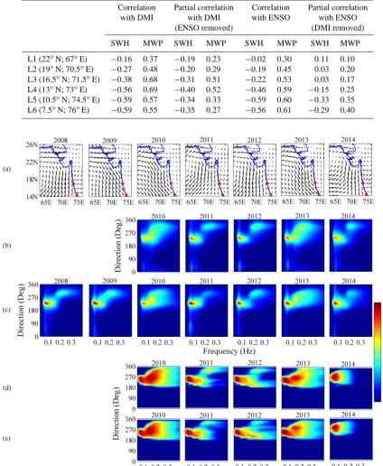
During October and November, the waves in the AS are dom-inated by low-amplitude (SWH < 1 m) wind seas (Young, 1994; Chempalayil et al., 2012; Glejin et al., 2013a), and dur-ing this time the DMI reaches its maximum value. For this particular period we examined the role of DMI on the wave climate of the eastern AS and observed that during October surface waves in this region show a response to DMI. We se-lected six locations (Fig. 1a) along the eastern AS which are at more than 100 km away from the coast of India (Table 1). The time series plot of SWH and mean wave period (MWP) with DMI are shown in Fig. 4a. Correlation and partial cor-relation of the wave parameters with DMI and SOI (southern oscillation index) are shown in Table 1 and this shows that SWH is negatively related and MWP is positively related to DMI. The influence of IOD increases towards the south, but after removing ENSO (SOI) the correlation values in all locations decrease and maximum correlation is observed in the central AS (location L4). This implies that if influences of ENSO are removed, then IODs have more impact on the central eastern AS than further north or south. The impact of ENSO with and without IOD was checked here and it is iden-tified that without the IOD, the impact of ENSO is significant
Figure 4. (a) Anomaly of significant wave height (SWH) and mean wave period (MWP) at six selected locations off the west coast of India during October from 1979 to 2014 along with DMI. The wave data are from ERA-I. Locations are shown in Fig. 1. (b) Plot of SST anomaly in the west and east equatorial IO. SST data are from Tropflux.
only in the southern part of the eastern AS. From this it is cer-tain that in the eastern AS region IOD has more impact than ENSO and its effect is dominant off the central west coast of India. The variability of SWH and MWP with respect to the DMI index from 1979 to 2013 is shown in time series plot at the same six locations (Fig. 4a). The anomaly in the SWH varies between−0.2 and 0.4 m and that for MWP from−2 to 1 s. Maximum SWH and MWP anomaly is observed during 1997, which is the strongest IOD year of the study period.
Table 1. Correlation and partial correlation of SWH and MWP with DMI and NINO3 time series during October, from 1979 to 2014.
Correlation Partial correlation Correlation Partial correlation with DMI with DMI with ENSO with ENSO
(ENSO removed) (DMI removed)
SWH MWP SWH MWP SWH MWP SWH MWP
L1 (22◦N; 67◦E) −0.16 0.37 −0.19 0.23 −0.02 0.30 0.11 0.10 L2 (19◦N; 70.5◦E) −0.27 0.48 −0.20 0.29 −0.19 0.45 0.03 0.20 L3 (16.5◦N; 71.5◦E) −0.38 0.68 −0.31 0.51 −0.22 0.53 0.03 0.17 L4 (13◦N; 73◦E) −0.56 0.69 −0.40 0.52 −0.46 0.59 −0.15 0.25 L5 (10.5◦N; 74.5◦E) −0.59 0.57 −0.34 0.33 −0.59 0.60 −0.33 0.35 L6 (7.5◦N; 76◦E) −0.59 0.55 −0.35 0.27 −0.56 0.61 −0.29 0.40
Figure 5. Averaged wind pattern of October from 2008 to 2014 (a). Averaged measured wave frequency–directional spectra from 2008 to 2014 off Ratnagiri (b) and off Honnavar (c). Color bar is for spectral energy (m2Hz−1Deg−1). (d) Modeled directional spectrum off Ratnagiri and (e) off Honnavar from 2010 to 2014. The spectral energy is shown in logarithmic scale base 10. SST anomalies of eastern and western equatorial IO with DMI are shown in Fig. 4.
are from the northerly direction and change to northwesterly before merging with the westerly equatorial winds and north-westerly winds nearer the Indian coast. This pattern of wind
Figure 6. Scatter plot of zonal wind within 14 to 20◦N and 70 to 73◦E with SWH of high-frequency range (0.14 to 0.29 Hz) and NW direction waves (280 to 320◦) off Honnavar (from 2008 to 2014) and off Ratnagiri (from 2010 to 2014).
Pure positive IOD and combined events are considered fol-lowing Aparna et al. (2012). A pure IOD event is that which occurs in the absence of an ENSO event (Rao et al., 2002). A positive (negative) IOD event that co-occurs with an El Niño (La Niña) is a combined IOD event. A pure ENSO event is defined similarly. The combined events are strong only if both El Niño and positive IOD events are strong. Figure 1c and d show the wind pattern during pure positive and combined IOD events respectively. As observed from climatology, these figures illustrate that in the eastern AS the northwesterly wind vectors are modified to northeast-erly. Instead of going towards the eastern equatorial IO the wind blows towards the western IO. This can be perceived as more strong in combined event of PIOD with a comparatively weak wind vectors along the southwest of India. During the negative IOD (NIOD) events (Fig. 1e and f) wind blows over the central and eastern AS as northwesterly which is in con-trast to the wind pattern during PIOD. This modification in the wind pattern over the central AS to either westward or eastward direction from its general climatology pattern dur-ing the PIOD or NIOD events is due to the IOD-induced tem-perature variability in the equatorial IO.
Measured frequency–directional spectra of surface waves from two locations off the central west coast of India are shown in Fig. 5. The wind pattern of corresponding years is shown in Fig. 5a and year wise SST anomaly in west, east and DMI index for October is shown in Fig. 4a and b. For the years 2008 to 2014, it can be seen that maximum positive DMI index is observed during 2011 (Fig. 4a). Dur-ing this year the wind in the eastern AS has shifted its di-rection to northeasterly. Its influence is clearly visible in the frequency–directional spectra of waves at Ratnagiri and Hon-navar, due to the decrease in short-period waves from the northwest (NW) direction. This difference in higher energy at Ratnagiri than Honnavar is clearly evident from Fig. 5b and c and is caused by the alteration of wind direction to the NE before reaching Honnavar. So the dissipation of NW waves and weak wind in the Honnavar region causes a decrease in
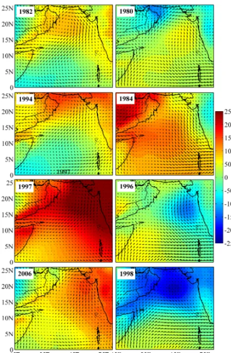
Figure 7. SST anomaly (◦C) of four strong positive (first column) and four negative (second column) IOD years from 1979 to 2014. Years are shown inside the figure and SST anomalies of eastern and western equatorial IO with DMI for corresponding years are shown in Fig. 4.
Figure 8. Wind vector (m s−1) and SLP anomaly (Pa) of four strong positive (first column) and four negative (second column) IOD years from 1979 to 2014. Years are shown inside the figure and SST anomalies of eastern and western equatorial IO with DMI for cor-responding years are shown in Fig. 4.
2008 is observed in 2009. However, the influences of high SST anomalies are not observed either in the wind pattern or wave climate. This shows that the modification of wind vec-tors not only depends on the SST anomaly in the west or east separately but also on the DMI index.
To confirm the influence of IOD-induced turning wind pat-tern (Fig. 1b to f) on the waves off the west coast of In-dia, we spatially averaged the zonal wind component within the region where wind shows alteration in its direction (14 to 20◦N; 70 to 73◦E) and averaged the short period waves within the 0.14–0.29 Hz frequency range and 280–320◦ di-rection. The scatter plot for both zonal wind and measured SWH in this particular direction and frequency range off Rat-nagiri and off Honnavar for all years are shown in Fig. 6. From the figure it can be seen that the zonal wind component in this region has a direct influence to the wave climate of this region. SWH increases with the zonal wind component,
and this increase is greater when the zonal wind component is positive than when it is negative.
During the negative phase of IOD, the swell height is slightly less than that during the positive phase (Fig. 5b and c). The turbulent sea state generated by the dom-inance of short-period waves during the negative phase of IOD leads to an increased decay rate of swell (Ardhuin et al., 2009; Young et al., 2013). The sign reversal of the air–sea momentum flux depends on a parameter known as inverse wave age (ratio of sea surface wind speed to the speed of the wave corresponding to peak frequency) and it is very use-ful to understand the present sea state (Grachev and Fairall, 2001; Hanley and Belcher, 2008; Hanley et al., 2010). Here, we calculated the monthly (October) average inverse wave age off Ratnagiri and the values are 0.32, 0.11, 0.27, 0.35 and 0.17 from 2010 to 2014. From this it is further evi-dent that during the positive phase of IOD, the eastern AS is a wave-driven wind region (inverse wave age < 0.15) – i.e., waves transfer momentum to wind. During the negative IOD period, the region becomes mixed state (0.15 < inverse wave age < 0.83; both wind-driven wave and wave-driven wind are present). The modeled frequency–directional spec-tra off Ratnagiri and Honnavar from 2010 to 2014 are shown in Fig. 5d and e. Comparison of measured and modeled spec-tra off Honnavar and Ratnagiri shows that the specspec-tral en-ergy is overestimated by the model since the ERA-I wind data used in the study are with a coarse resolution of 1◦×1◦ (Fig. 5b and c). Even though the model overestimated the spectral energy, it can be observed that the model reproduced almost the same pattern as the observed wave spectra. The influence of altering wind pattern is clearly evident in the modeled spectra as well.
Since IOD has large influence on SST variability in equa-torial IO, here we show the SST of AS and western equaequa-torial Indian Ocean in Fig. 7. We considered comparatively strong PIOD and NIOD events from 1979 to 2014. The PIOD years are 1982, 1994, 1997 and 2006 (left panel of Fig. 7). Among these in 1994, IOD occurs in the absence of ENSO. The NIOD years are 1980, 1984, 1996 and 1998 (right panel). This SST variability produces variability in SLP (Fig. 8). The wind pattern of the respective years for AS and part of equa-torial IO are shown in the same figure. Since the NIOD is the intensification of the normal condition of October (Vinay-achandran et al., 2009), the SLP in the western equatorial IO is higher and lower in the eastern equatorial IO. Hence, the winds from the northern AS will propagate towards the east-ern equatorial IO along the easteast-ern AS. This shows the in-fluence of IOD-induced temperature variability on SLP and wind direction.
Figure 9. Modeled directional spectrum off Honnavar and Ratnagiri for selected positive and negative IOD years (first and third columns for positive IOD and second and fourth columns for negative IOD). Corresponding years are shown inside the figures and DMI are shown in Fig. 4. The spectral energy is shown in logarithmic scale base 10.
respectively; similarly the second and fourth columns are for NIOD years. From the figure it is evident that for the positive phase of IOD, the short-period waves from the NW direc-tion are less at both locadirec-tions, whereas 2006 shows a con-flicting result. From Fig. 8, it is clear that in 2006 the wind pattern in the central AS is northeasterly as observed in the other PIOD events, but along the eastern AS the wind vector extends slightly further south compared to the strong events observed during 1994 and 1997. A similar pattern, but com-paratively less spatial extension in wind vectors towards the south, is also evident during 1982 (Fig. 8).
In the case of 1996, which is the strongest NIOD event considered in this study, we expect a more evident signature in SWH at the study locations of Ratnagiri and Honnavar. However, in the wave spectrum its signature is weaker than that observed in 1980 and 1984 (Fig. 9). The wind pattern ob-served during the period, in 1996, is northerly down to 15◦N then it turns northwesterly and propagates towards the east-ern equatorial IO (Fig. 8). The change in wind patteast-ern from the composite climatology of NIOD events (Fig. 1e and f) causes the weakening of short-period waves arriving from the NW and corresponding influence in the directional wave spectra. Similarly, the second strongest NIOD event occurred
in 1998, but the signature of this event is absent in the wave climate. The northern–eastern AS region is calm due to the absence of NW winds in the northern AS, in turn due to the associated negative SLP anomaly.
4 Conclusions
field over the central and south-of-central west coast of India. This change in direction of wind pattern in the AS causes a decrease in wave height off the central and southwest coast of India during PIOD, whereas during NIOD events the wind vector turns to northwesterly instead of northerly winds in the composite climatology over the region during October. This leads to an increase of short-period waves in the same region. The influence of IOD on the wave climate mainly de-pends on the modification of wind field caused by the phases of IOD event. If this wind pattern is absent even during a strong IOD event, then the signature of the IOD on the wave climate is also absent. This alteration of wind pattern mainly depends on the IOD-induced SST variability in the eastern and western equatorial IO, and some other unknown factors may also cause slight modification in this wind – more anal-ysis is required to understand this variability. From this study it is clear that IOD has an impact on the wave climate off the west coast of India especially off the central west coast of In-dia due to the decrease of northwesterly short-period waves.
Acknowledgements. The authors acknowledge the CSIR, New Delhi for funding the wave measurement at Honnavar and ESSO-INCOIS, Ministry of Earth Sciences, Government of India for funding the wave measurement at Ratnagiri. The director of CSIR-NIO, Goa provided encouragement to carry out the study. The deep water buoy data used for validation of the numerical model were collected by the National Institute of Ocean Tech-nology, Chennai and provided by the Indian National Centre for Ocean Information Services (INCOIS) Ministry of Earth Sciences, Hyderabad. T. M. Balakrishnan Nair, A. Nherakkol and J. Singh provided support during data collection. We thank A. Vedpathak and P. Kulkarni, Centre for Coastal & Marine Biodiversity, Dr. Babasaheb Ambedkar Marathwada University, Ratnagiri for providing the logistics required for wave data collection at Ratna-giri. This work forms part of the Ph.D. thesis of the first author. We thank the topic editor J. M. Huthnance and the two reviewers for their critical review and suggestions, which improved the sci-entific content of the paper. This work is NIO contribution no. 5866.
Edited by: J. M. Huthnance
References
Aboobacker, V. M., Rashmi, R., Vethamony, P., and Menon, H. B.: On the dominance of pre-existing swells over wind seas along the west coast of India, Cont. Shelf Res., 31, 1701–1712, 2011. Amante, C. and Eakins, B. W.: ETOPO1 1 arc-minute global
re-lief model: procedures, data sources and analysis, NOAA Tech. Memo., NESDIS NGDC-24, National Oceanic and Atmospheric Administration, Boulder, Colorado, USA, 19 pp., 2009. Amrutha, M. M., Sanil Kumar, V., and Singh, J.: Changes in
nearshore waves during the active sea/land breeze period off Ven-gurla, central west coast of India, Ann. Geophys., 34, 215–226, doi:10.5194/angeo-34-215-2016, 2016.
Anoop, T. R., Kumar, V. S., Shanas, P. R., and Johnson, G.: Surface wave climatology and its variability in the North Indian Ocean
based on ERA-Interim reanalysis, J. Atmos. Ocean. Tech., 32, 1372–1385, doi:10.1175/JTECH-D-14-00212.1, 2015.
Aparna, S. G., McCreary, J. P., Shankar, D., and Vinayachan-dran, P. N.: Signatures of Indian Ocean Dipole and El Niño–Southern Oscillation events in sea level variations in the Bay of Bengal, J. Geophys. Res.-Oceans, 117, C10012, doi:10.1029/2012JC008055, 2012.
Ardhuin, F., Chapron, B., and Collard, F.: Observation of swell dissipation across oceans, Geophys. Res. Lett., 36, L06607, doi:10.1029/2008GL037030, 2009.
Baquero-Bernal, A., Latif, M., and Legutke S.: On dipole like vari-ability of sea surface temperature in the tropical Indian Ocean, J. Climate, 15, 1358–1368, 2002.
Booij, N., Ris, R. C., and Holthuijsen L. H.: A third-generation wave model for coastal regions: 1. Model description and vali-dation, J. Geophys. Res.-Oceans, 104, 7649–7666, 1999. Bunney, C.: A high resolution SWAN model assessment: North
Norfolk to Humber, Forecasting Research Technical Report 557, Met Office, Devon, UK, 2011.
Chempalayil, S. P., Sanil Kumar, V., Johnson, G., Udhaba, D. G., and Vinayaraj, P.: Interannual and seasonal variations in nearshore wave characteristics off Honnavar, west coast of India, Curr. Sci. India, 103, 286–292, 2012.
Dee, D. P., Uppala, S. M., Simmons, A. J., Berrisford, P., Poli, P., Kobayashi, S., and Vitart F.: The ERA-Interim reanalysis: Con-figuration and performance of the data assimilation system, Q. J. Roy. Meteor. Soc., 137, 553–597, 2011.
Endo, S. and Tozuka, T.: Two flavors of Indian Ocean Dipole, Clim. Dynam., 1–15, doi:10.1007/s00382-015-2773-0, 2015.
Grachev, A. A. and Fairall, C. W.: Upward momentum transfer in the marine boundary layer, J. Phys. Oceanogr., 31, 1698–1711, 2001.
Hanley, K. E. and Belcher, S. E.: Wave-driven wind jets in the ma-rine atmospheric boundary layer, J. Atmos. Sci., 65, 2646–2660, 2008.
Hanley, K. E., Belcher, S. E., and Sullivan, P. P.: A global clima-tology of wind-wave interaction, J. Phys. Oceanogr., 40, 1263– 1282, 2010.
Glejin, J., Sanil Kumar, V., Sajiv, P. C., Singh, J., Pednekar, P., Ku-mar, K. A., Dora, G. U., and Gowthaman, R.: Variations in swells along eastern Arabian Sea during the summer monsoon, Open Journal of Marine Science, 2, 43–50, 2012.
Glejin, J., Sanil Kumar, V., Balakrishnan Nair, T. M., and Singh, J.: Influence of winds on temporally varying short and long period gravity waves in the near shore regions of the eastern Arabian Sea, Ocean Sci., 9, 343–353, doi:10.5194/os-9-343-2013, 2013a. Glejin, J., Sanil Kumar, V., Nair, T. M. B., Singh, J., and Mehra P.: Observational Evidence of Summer Shamal Swells along the West Coast of India, J. Atmos. Ocean. Tech., 30, 379–388, 2013b.
Glejin, J., Sanil Kumar, V., and Nair, T. M. B.: Monsoon and cyclone induced wave climate over the near shore waters off Puduchery, south western Bay of Bengal, Ocean Eng., 72, 277– 286, 2013c.
(JON-SWAP), Deutsche Hydrographische Zeitschrift, Supplement A., 8, 95 pp., 1973.
Hastenrath, S. and Polzin, D.: Dynamics of the surface wind field over the equatorial Indian Ocean, Q. J. Roy. Meteor. Soc., 130, 503–517, 2004.
Komen, G., Hasselmann, S., and Hasselmann, K.: On the existence of a fully developed wind-sea spectrum, J. Phys. Oceanogr., 14, 1271–1285, 1984.
Kumar, B. P., Vialard, J., Lengaigne, M., Murty, V. S. N., and McPhaden, M. J.: TropFlux: air-sea fluxes for the global tropi-cal oceans-description and evaluation, Clim. Dynam., 38, 1521– 1543, 2012.
Kumar, B. P., Vialard, J., Lengaigne, M., Murty, V. S. N., McPhaden, M. J., Cronin, M. F., Pinsard, F., and Reddy, K. G.: TropFlux wind stresses over the tropical oceans: evaluation and comparison with other products, Clim. Dynam., 40, 2049–2071, 2013.
Murtugudde, R., McCreary, J. P., and Busalacchi A. J.: Oceanic pro-cesses associated with anomalous events in the Indian Ocean with relevance to 1997–1998, J. Geophys. Res.-Oceans, 105, 3295–3306, 2000.
Neetu, S., Shetye, S. R., and Chandramohan, P.: Impact of sea breeze on wind-seas off Goa, west coast of India, J. Earth Syst. Sci., 115, 229–234, 2006.
Premkumar, K., Ravichandran, M., Kalsi, S. R., Sengupta, D., and Gadgil, S.: First results from a new observational system over the Indian Seas, Curr. Sci. India, 78, 323–330, 2000.
Rao, A. S., Behera, S. K., Masumoto, Y., and Yamagata, T.: Inter-annual subsurface variability in the tropical Indian Ocean with a special emphasis on the Indian Ocean Dipole, Deep Sea Res. Pt. II, 49, 1549–1572, 2002.
Reverdin, G.: Convergence in the equatorial surface jets of the In-dian Ocean, J. Geophys. Res.-Oceans, 90, 11741–11750, 1985. Ris, R. C., Holthuijsen, L. H., and Booij, N.: A third-generation
wave model for coastal regions 2. Veri?cation, J. Geophys. Res.-Oceans, 104, 7667–7681, 1999.
Saji, N. H. and Yamagata, T.: Structure of SST and Surface Wind Variability during Indian Ocean Dipole Mode Events: COADS Observations, J. Climate, 16, 2735–2751, 2003.
Saji, N. H., Goswami, B. N., Vinayachandran, P. N., and Yamagata, T.: A dipole mode in the tropical Indian Ocean, Nature, 401, 360– 363, 1999.
Sanil Kumar, V. and Anjali Nair, M.: Inter-annual variations in wave spectral characteristics at a location off the central west coast of India, Ann. Geophys., 33, 159–167, doi:10.5194/angeo-33-159-2015, 2015.
Sanil Kumar, V. and Naseef, T. M.: Performance of ERA-Interim wave data in the nearshore waters around India, J. Atmos. Ocean. Tech., 32, 1257–1269, 2015.
Sanil Kumar, V., Shanas, P. R., and Dubhashi, K. K.: Shallow water wave spectral characteristics along the eastern Arabian Sea, Nat. Hazards, 70, 377–394, 2014.
Shanas, P. R. and Sanil Kumar, V.: Temporal variations in the wind and wave climate at a location in the eastern Arabian Sea based on ERA-Interim reanalysis data, Nat. Hazards Earth Syst. Sci., 14, 1371–1381, doi:10.5194/nhess-14-1371-2014, 2014. Shinoda T. and Han, W.: Influence of the Indian Ocean dipole on
atmospheric sub seasonal variability, J. Climate, 18, 3891–3909, 2005.
Slingo, J. M. and Annamalai, H.: The El Nino of the century and the response of the Indian summer monsoon, Mon. Weather Rev., 128, 1778–1797, 2000.
Sreenivas, P., Gnanaseelan C., and Prasad, K. V. S. R.: Influence of El Niño and Indian Ocean Dipole on sea level variability in the Bay of Bengal, Global Planet. Change., 80, 215–225, 2012. Tolman, H. L.: A third-generation model for wind waves on slowly
varying, unsteady and inhomogeneous depths and currents, J. Phys. Oceanogr., 21, 782–797, 1991.
Tolman, H. L.: User manual and system documentation of WAVE-WATCH III TM version 3.14. Tech. Note., 276, National Oceanic and Atmospheric Administration, National Weather Service, Maryland, USA, 194 pp., 2009.
Tolman, H. L. and Chalikov, D.: Source terms in a third-generation wind wave model. J. Phys. Oceanogr., 26, 2497–2518, 1996. Uppala, S. M., Kållberg, P. W., Simmons, A. J., Andrae, U.,
Bechtold, V., Fiorino, M., and Woollen, J.: The ERA-40 re-analysis, Q. J. Roy. Meteor. Soc., 131, 2961–3012, 2005. Vinayachandran, P. N., Francis, P. A., and Rao, S. A.: Indian Ocean
dipole: processes and impacts, Current Trends in Science: Plat-inum Jubilee Special, Indian Academy of Sciences Bangalore, 569-589, 2009.
Webster, P. J., Moore, A. M., Loschnigg, J. P., and Leben, R. R.: The great Indian Ocean warming of 1997–1998: Evidence of coupled oceanic-atmospheric instabilities, Nature, 401, 356–360, 1999. Wyrtki, K.: Oceanographic Atlas of the International Indian Ocean
Expedition, Natl. Sci. Found., Washington, D.C., Usa. 531 pp., 1971.
Young, I. R.: Global ocean wave statistics obtained from satellite observations, Appl. Ocean. Res., 16, 235–248, 1994.
Young, I. R., Babanin, A. V., and Zieger, S.: The decay rate of ocean swell observed by altimeter, J. Phys. Oceanogr., 43, 2322–2333, 2013.