Data assimilation for plume models

(1)

Nonlinear Processes in Geophysics (2005) 12: 257–267 SRef-ID: 1607-7946/npg/2005-12-257

European Geosciences Union

Nonlinear Processes

in Geophysics

Data assimilation for plume models

C. A. Hier Majumder1, 4, E. B´elanger2, S. DeRosier3, 4, *, D. A. Yuen3, 4, and A. P. Vincent2

1_{Computational Physics Group, Earth Science Division, Lawrence Livermore National Laboratory, Livermore, CA, USA} 2_{Département de Physique, Université de Montréal, Montréal, Québec, Canada}

3_{Department of Geology and Geophysics, University of Minnesota, Minneapolis, Minnesota, USA} 4_{Minnesota Supercomputing Institute, University of Minnesota, Minneapolis, Minnesota, USA}

*_{now at: Department of Earth and Space Sciences, University of Washington, Seattle, Washington, USA}

Received: 9 August 2004 – Revised: 7 December 2004 – Accepted: 8 December 2004 – Published: 9 February 2005

Abstract. We use a four-dimensional variational data

assim-ilation (4D-VAR) algorithm to observe the growth of 2-D plumes from a point heat source. In order to test the pre-dictability of the 4D-VAR technique for 2-D plumes, we per-turb the initial conditions and compare the resulting predic-tions to the predicpredic-tions given by a direct numerical simula-tion (DNS) without any 4D-VAR correcsimula-tion. We have stud-ied plumes in fluids with Rayleigh numbers between 106and 107and Prandtl numbers between 0.7 and 70, and we find the quality of the prediction to have a definite dependence on both the Rayleigh and Prandtl numbers. As the Rayleigh number is increased, so is the quality of the prediction, due to an increase of the inertial effects in the adjoint equations for momentum and energy. The horizon predictability time, or how far into the future the 4D-VAR method can predict, decreases as Rayleigh number increases. The quality of the prediction is decreased as Prandtl number increases, how-ever. Quality also decreases with increased prediction time.

1 Introduction

Scientists often do not know the exact initial conditions for a numerical simulation. For example, a meteorologist can never know the exact state of the atmosphere at a given time. Therefore, there will always be errors in the initial condi-tions for meteorological forecasts (Daley, 1991). Due to the instability of the atmosphere with respect to small amplitude perturbations, two slightly different states may evolve into appreciably different states (Lorenz, 1982). This means that atmospheric forecasts have an intrinsic upper bound to pre-dictability of about two weeks (Lorenz, 1984). Similarly, geophysicists cannot know the exact position of the conti-nents in the past, nor the full temperature and velocity fields at a given instant. Consequently, any numerical simulation of mantle convection will always have uncertainties in the initial conditions (Bunge et al., 2003; Ismail-Zadeh et al., 2004). It

Correspondence to: C. A. Hier Majumder

([email protected])

is even difficult to set initial conditions for simulations mod-eling the behavior of individual plumes in the present mantle since tomographic data can be noisy, and the resolution can vary greatly with location.

The effect of inaccurate initial conditions can be decreased using variational data assimilation (Courtier et al., 1993). This method was developed by meteorologists to increase the accuracy of weather predictions (Daley, 1991). Using the adjoint equations allows the simulation to move back-ward in time to correct inaccuracies in the initial conditions (Courtier, 1997; Errico, 1997). For example, a weather fore-cast is started with a set of initial conditions. These initial conditions consist of measurements of the state of the atmo-sphere and oceans at a given time. As the simulation is com-puted, the meteorologists continue to collect more weather data at future times. Variational data assimilation allows them to add these observations into the model. The simu-lation can then move backward in time to correct the old ini-tial conditions and give results closer to the new observations when the model reaches the point in time at which the new observations were taken. This method allows meteorologists to continually improve the data integrated into the simulation with time and leads to more accurate forecasts. It also allows data that occurs after the analysis time to be integrated into the simulation (Zhu et al., 2003). For example, in climate research one would want to integrate observations about the present state of the atmosphere into a model that provides information about the past state of the atmosphere.

(2)

258 C. A. Hier Majumder et al.: Data assimilation for plume models The adjoint equations have also been used to find the

thermal state of the Earth’s mantle in the mid-Cretaceous (100 mya) (Bunge et al., 2003). This mantle study begins with the present state of the mantle as known from seismic tomography. It then moves backward and forward in time while using variational data assimilation to incorporate data from past plate motions and decrease the residuals. The cor-rection process becomes stationary after 100 iterations, and the final output is a thermal picture of the mantle 100 mya.

Four-dimensional variational data assimilation (4D-VAR) takes advantage of the powers of both the adjoint equations and variational data assimilation. It uses a periodic update of the adjoint sensitivity field to integrate time distributed ob-servations into the simulation (Daescu and Navon, 2003). It has been used in simulations of floods in river and dam sys-tems (B´elanger and Vincent, 2005; B´elanger et al., 2003). These simulations need river height as an initial condition. The river height, however, can be quite variable due to pre-cipitation and water discharge throughout the watershed. It is impossible to know in advance the exact river height this type of system will experience. Therefore, the initial river height used is always erroneous. With variational data assimilation the modeler can develop a simulation that is less dependent on the error in the initial river height.

This study focuses on the behavior of thermal plumes. Plumes of type are important to a wide variety of phenomena, including mantle convection (Kaminski and Jaupart, 2003; Lithgow-Bertelloni et al., 2001), deep sea thermals (Lavelle, 1997), solar convection (Rast, 1998, 2000), and fires (Cete-gen et al., 1998). Many advances have been made in the past ten years on the development of laboratory experimen-tal techniques for the study of finite Prandtl plumes (Moses et al., 1993; Cetegen et al., 1998; Lithgow-Bertelloni et al., 2001; Kaminski and Jaupart, 2003). The 4D-VAR technique discussed here can be used as an optimal control tool to allow experimentalists to check their ongoing experiments in real time or even as a prediction technique to help determine the expected behavior at some future time. Although the method developed here deals with finite Prandtl plumes, it can be eas-ily adpated for use with the infinite Prandtl equations. This would allow the technique to be used to incorporate seismic tomography data available for mantle plumes (Montelli et al., 2004; Zhao, 2001) into numerical models.

The goal of our study is to use the 4D-VAR method to prove that we can predict the behavior of turbulent, finite-Prandtl plumes even if we do not have a complete knowledge of their initial conditions. We know both the initial and final states of a plume with a defined set of initial conditions. We call this data our “observations”. We take our defined initial conditions and add a small error to them. We then use the 4D-VAR method to test whether we can predict the behavior of the plume using the erroneous initial conditions. We refer to the plume calculated from the erroneous initial conditions as the “forecast” or “prediction”. For a given time, we iter-ate forward/backward and look at the residuals between the observation and forecast after the iterations are done. We vary the time to test how long we can accurately predict the

behavior of a plume whose initial conditions are not exactly known. We vary the Rayleigh number from 1×106to 3×107 and the Prandtl number from 0.7 to 70 in order to test how the predictability changes with Rayleigh and Prandtl number.

2 The 4D-VAR technique and the equations of the plume

The 4D-VAR variational assimilation method can be de-scribed in the following way. First, a cost function is con-ceived to measure the error between the forecast and the ob-servations (Talagrand and Courtier, 1987). Then the adjoint equations, which are used to evaluate the gradient of this cost function, are obtained by applying a variational procedure to the Lagrangian problem (Courtier et al., 1993). The cost function and its gradient are minimized by a minimization algorithm, such as the steepest descent (Burden and Faires, 1993), in order to find the optimal initial conditions that will give the optimal forecast.

2.1 The cost function

When using a variational method, it is necessary to write the problem as a functional that one wants to minimize. This functional is known as the cost function. It is a measure of the error between the observations and predictions that one wants to minimize. In general, the cost function is written:

J = Z t2

t1 Z

f (−→9 ,x, t ) dxdt, (1)

wheref (9,x, t )is a scalar function defined on a domain,

, and a time interval, [t1, t2] (Sanders and Katopodes,

2000).f (9,x, t )is a function of9that represents the state variables, such as the speed or the temperature. In this study, the cost function used is:

J =1 2

Z

Z t2

t1

(Hcal−Hobs)(Hcal−Hobs)dt dx, (2)

whereHcalis the forecasted convective heat flux, andHobsis

the observed convective heat flux. The heat flux is calculated at each grid point by taking the vertical velocity,vz, and the temperature,T:

H =vzT . (3)

Our cost function is similar to the objective functional of the temperature used by Ismail-Zadeh et al. (2004) except that we took into account errors in both the velocity and temper-ature field by using the heat flow.

2.2 The adjoint equations

(3)

C. A. Hier Majumder et al.: Data assimilation for plume models 259 Usually, when trying to solve a problem with constraints,

one uses the Lagrangian. The formulation of the undeter-mined Lagrangian multipliers are constructed for the system that one wants to study:

L(−→9 ,−→λ )=J (−→9 )+ Z t2

t1 Z

− →

λ (x, t )·E(−→9 ,x, t ) dxdt,(4) whereJ (9)is the cost function andλ(x, t )are the unde-termined Lagrangian multipliers, also called the adjoint vari-ables (Sanders and Katopodes, 1999). It has been demon-strated that finding the stationary point of the cost function with the constraints E(9,x, t )=0 is equivalent to finding the stationary points of the Lagrangian with respect of9and λ(Dimet and Talagrand, 1986).

When we minimize the Lagrangian, the stationary points that we want to find are saddle points; rather than the abso-lute maximums or minimums (Dimet and Talagrand, 1986). In order to accomplish this task, we will apply the variational operatorδto the Lagrangian. Here, the displacement direc-tions are the physical variables of the system as well as the adjoint variables. Taking the variation of the Lagrangian, we obtain:

δL=−→∇ −→

9L·δ

− →

9 +−→∇ −→

λL·δ

− →

λ

= ∂L

∂−→9δ

− →

9 + ∂L

∂−→λ δ

− →

λ . (5)

Also note that we have linearized the problem in the same step (Ehrendorfer, 1992). For an arbitrary displacement

(δ9, δλ), we are at a minimum only ifδL=0 (Daley, 1991). This indicates that the derivative of the Lagrangian with re-spect to each direction must be zero:

∂L

∂−→λ

=E(−→9 ,x, t )=0 (6)

and

∂L

∂−→9

=Adj(−→λ )+ ∂J

∂−→9

=0, (7)

where Adj(λ)represents the adjoint equations after integra-tion by parts (Schr¨oter et al., 1993). Note that Eq. (6) is the system of equations that one had at the beginning and that Eqs. (6) and (7) are the Euler-Lagrange equations (Dimet and Talagrand, 1986).

Unfortunately, an efficient means for directly solving the Euler-Lagrange equations does not exist. This situation forces us to reformulate our problem to one without con-straints (Talagrand and Courtier, 1987). Since the physical equations of the model are deterministic, it is evident that the state of the system at the time of the observations depends only on the initial conditions,90, of the system. Therefore,

the cost function is an implicit function of the initial condi-tions. It is by varying the initial conditions that we will solve the physical equations while minimizing the cost function (Ehrendorfer, 1992). According the theory of optimal con-trol (Lions, 1968), the concon-trol variables of the problem are

C. A. Hier Majumder et al.: Data Assimilation for Plume Models

3

physical equations

J K,

1 "%#%$

, which act as the

con-straints. Therefore, this is a problem of minimization with

constraints (Talagrand and Courtier, 1987).

Usually, when trying to solve a problem with constraints,

one uses the Lagrangian. The formulation of the

undeter-mined Lagrangian multipliers are constructed for the system

that one wants to study:

L M

N $

O P% Q$SR

N

"!#%$T

J

%

M1 U%#%$S&* &*#

(4)

where

<-,

$

is the cost function and

V

"%#%$

are the

unde-termined Lagrangian multipliers, also called the adjoint

vari-ables (Sanders and Katopodes, 1999). It has been

demon-strated that finding the stationary point of the cost function

with the constraints

J

-,

! "%#%$

is equivalent to finding

the stationary points of the Lagrangian with respect of

,

and

V

(Dimet and Talagrand, 1986).

When we minimize the Lagrangian, the stationary points

that we want to find are saddle points; rather than the

abso-lute maximums or minimums (Dimet and Talagrand, 1986).

In order to accomplish this task, we will apply the variational

operator

W

to the Lagrangian. Here, the displacement

direc-tions are the physical variables of the system as well as the

adjoint variables. Taking the variation of the Lagrangian, we

obtain:

W

L

X

L

T

W

YR

X

N

L

T

W

N

[Z

L

Z

W

\R

Z

L

Z

N

W

N

(5)

Also note that we have linearized the problem in the same

step (Ehrendorfer, 1992). For an arbitrary displacement

W

,

WHV

$

, we are at a minimum only if

W L

(Daley,

1991). This indicates that the derivative of the Lagrangian

with respect to each direction must be zero:

Z

L

Z

N

J

1 "%#%$

(6)

and

Z

L

Z

Adj

N $]R

Z

(7)

where Adj

V

$

represents the adjoint equations after

integra-tion by parts (Schr¨oter et al., 1993). Note that Eq. 6 is the

system of equations that one had at the beginning and that

Eqs. 6 and 7 are the Euler-Lagrange equations (Dimet and

Talagrand, 1986).

Unfortunately, an efficient means for directly solving the

Euler-Lagrange equations does not exist. This situation

forces us to reformulate our problem to one without

con-straints (Talagrand and Courtier, 1987). Since the physical

equations of the model are deterministic, it is evident that the

state of the system at the time of the observations depends

only on the initial conditions,

,_^

, of the system. Therefore,

the cost function is an implicit function of the initial

condi-tions. It is by varying the initial conditions that we will solve

the physical equations while minimizing the cost function

●Direct simulation New initial conditions

Adjoint equations ( J)

●

●Output: optimal forecast ●

●Output: first forecast (DNS) Direct simulation ●Read initial conditions

●

Cost function (J) ∆ ●

Read observations

●Minimization (steepest descent)

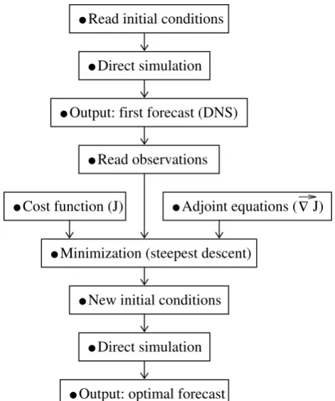
Fig. 1.

Algorithm for the 4D-VAR method.

(Ehrendorfer, 1992). According the theory of optimal

con-trol (Lions, 1968), the concon-trol variables of the problem are

the initial conditions. One can also use the boundary

condi-tions as control variables (Schr¨oter et al., 1993). In our

prob-lem, we have removed the constraints since no restrictions

are applied to the initial conditions.

Finally, the gradient of the cost function (Eq. 2) with

re-spect to the initial vertical heat flux is given by the adjoint

variables evaluated at time

`

# 3

(Courtier, 1997):

ab *c2defhgHi 1jk

`

#3I$

(8)

a *lmden g oi 1jk

`

# 3 $

(9)

ab *p*derq+gHoi !j

`

# 3 $

(10)

ab *s2de

F

g oi !j

`

# 3 $

(11)

2.3 The 4D-VAR data assimilation algorithm

Starting from initial conditions obtained by current

exper-imental observations or a previous numerical simulation,

a direct simulation generates a traditional (DNS) forecast

(Fig. 1). After reading the observations taken at the end of

the forecast period, the initial error between the forecast and

the observations is calculated. This initial error will provide

a first guess to a minimization algorithm.

In this theoretical study, we needed to vary the

accu-racy and the input parameters to test the 4D-VAR

tech-nique. Since we were testing the validity of the technique,

we did not use real data. Many experimental studies have

been conducted on the behavior of finite Prandtl number

plumes (Kaminski and Jaupart, 2003; Lithgow-Bertelloni

et al., 2001; Cetegen et al., 1998; Moses et al., 1993). The

4D-VAR method introduced here will allow integration of

experimental studies into numerical models. The technique

Fig. 1. Algorithm for the 4D-VAR method.

the initial conditions. One can also use the boundary condi-tions as control variables (Schr¨oter et al., 1993). In our prob-lem, we have removed the constraints since no restrictions are applied to the initial conditions.

Finally, the gradient of the cost function (Eq. 2) with re-spect to the initial vertical heat flux is given by the adjoint variables evaluated at timeτ=t2(Courtier, 1997):

∇Ju0 =u ∗

(x, z, τ =t2) (8)

∇Jw0 =w ∗

(x, z, τ =t2) (9)

∇JP0 =P ∗

(x, z, τ =t2) (10)

∇JT0 =T ∗

(x, z, τ =t2). (11)

2.3 The 4D-VAR data assimilation algorithm

Starting from initial conditions obtained by current exper-imental observations or a previous numerical simulation, a direct simulation generates a traditional (DNS) forecast (Fig. 1). After reading the observations taken at the end of the forecast period, the initial error between the forecast and the observations is calculated. This initial error will provide a first guess to a minimization algorithm.

(4)

260 C. A. Hier Majumder et al.: Data assimilation for plume models et al., 2001; Cetegen et al., 1998; Moses et al., 1993). The

4D-VAR method introduced here will allow integration of experimental studies into numerical models. The technique could also be used to incorporate the tomographic data avail-able of mantle plumes (Montelli et al., 2004; Zhao, 2001).

For the data assimilation run, we have perturbed the ini-tial conditions with a sinusoidal function. A direct simula-tion with the perturbed initial condisimula-tions permits us to obtain a simple forecast. After reading the observations (obtained previously), we calculate the initial error between the fore-cast and the observations. Then, we use a minimization algo-rithm, such as the steepest descent, in order to minimize the cost function (Eq. 2) with the aid of its gradient (Sect. 2.2). When the minimum has been found, we have the new initial conditions. These initial conditions are optimal because a second direct simulation using them will be an optimal fore-cast. The final error between this forecast and the observa-tions will be minimal.

2.4 The direct equations for a localized thermal plume The physical equations describing Rayleigh-B´enard convec-tion with the Boussinesq approximaconvec-tion that we used are:

∇·v=0 (12)

∂v

∂t =v×ω−∇P +

1 Re∇

2_v₊_T_e_ˆ

z (13)

∂T

∂t = −v·∇T +

1 Pe∇

2_{T ,} ₍₁₄₎

whereωis the vorticity (Hier Majumder et al., 2004). The equations have been nondimensionalized with the free-fall velocity:

U=pαg1T Lz, (15)

whereαis the coefficient of thermal expansion,gis the grav-itational acceleration, 1T is the initial temperature differ-ence between the heating point and the surrounding fluid, andLz is the box height. The Rayleigh (Ra) and Prandtl (P r) numbers are the nondimensional numbers often used in thermal convection equations. We defineRaas:

Ra= gα1T L

3

z

κν , (16)

whereκis the thermal diffusivity andνis the kinematic vis-cosity. The Prandtl number is defined as:

P r =ν

κ. (17)

The nondimensional numbers that appear in Eqs. (13) and (14) are the Reynolds number:

Re=U Lz

ν (18)

and the P´eclet number:

P e= U Lz

κ (19)

(Tritton, 1988). TheReandP eare related to the Rayleigh number (Ra) and the Prandtl number (P r) of the plume by:

Ra=P eRe (20)

and

P r =P e

Re. (21)

2.5 The adjoint equations for a localized thermal plume Following the method in Sect. 2.2, we obtained the adjoint equations (Marchuk, 1995):

∂u∗

∂τ =v·∇u

∗₋

u∂w

∗

∂z +w ∂w∗

∂x +

1 Re∇

2_u∗₊

u∇2P∗

−2u∂

2_P∗

∂x2 −2w

∂2P∗ ∂x∂z +T

∂T∗ ∂x −

∂J

∂u (22)

∂w∗

∂τ =v·∇w

∗₊

u∂u

∗

∂z −w ∂u∗

∂x +

1 Re∇

2_w∗₊

w∇2P∗

−2u∂

2_P∗

∂x∂z −2w ∂2P∗

∂z2 +T

∂T∗ ∂z −

∂J

∂w (23)

∇2P∗= ∂u ∗

∂x + ∂w∗

∂z − ∂J

∂P (24)

∂T∗

∂τ =v·∇T

∗₊ 1 Pe∇

2_T∗₊_w∗₋∂P ∗

∂z − ∂J

∂T, (25)

whereτ=t2−tis the inverse time. The initial conditions are:

δu(x, z, t|_t

1)=0 u∗(x, z, t|t2)=0

δv(x, z, t|_t

1)=0 v∗(x, z, t|t2)=0

δT (x, z, t|_t

1)=0 T ∗(x, z, t|t2)=0 (26) and the boundary conditions are:

u∗(0, z, t )=0 u∗(Lx, z, t )=0

v∗(0, z, t )=0 v∗(Lx, z, t )=0

T ∗(0, z, t )=0 T ∗(Lx, z, t )=0

P ∗(0, z, t )=0 P ∗(Lx, z, t )=0 (27)

u∗(x,0, t )=0 u∗(x, Lz, t )=0

v∗(x,0, t )=0 v∗(x, Lz, t )=0

T ∗(x,0, t )=0 T ∗(x, Lz, t )=0

P ∗(x,0, t )=0 P ∗(x, Lz, t )=0 (28)

∂u∗ ∂x

x=0

=0 ∂u

∗

∂z

z=0

=0

∂v∗ ∂x

_x₌₀

=0 ∂v

∗

∂z

_z₌₀

=0

∂P∗ ∂x

x=0

=0 ∂P

∗

∂z

z=0

=0

∂T∗ ∂x

x=0

=0 ∂T

∗

∂z

z=0

(5)

C. A. Hier Majumder et al.: Data assimilation for plume models 261

∂u∗ ∂x

x=Lx

=0 ∂u

∗

∂z

z=Lz

=0

∂v∗ ∂x

_x₌_L

x

=0 ∂v

∗

∂z

_z₌_L

z

=0

∂P∗ ∂x

_x₌_L

x

=0 ∂P

∗

∂z

_z₌_L

z

=0

∂T∗

∂x

x=Lx

=0 ∂T

∗

∂z

z=Lz

=0. (29)

3 Prediction: what can be expected for the 4D-VAR?

We start with a plume defined by a temperature and velocity field (Fig. 2a). We use this temperature and velocity field as exact initial conditions for a DNS. We save the temperature and velocity field at each iteration of the DNS to create the observations. We then take the plume defined by the exact initial conditions from the DNS and perturb its convective heat flux. This perturbation produces an error in the initial temperature and velocity fields that needs to be corrected by the 4D-VAR technique (Fig. 2b). The same perturbation is used for all Rayleigh and Prandtl numbers. A grid size of 64×192 is used for all runs. The timestep and number of iterations is set optimal for a given run. The 4D-VAR al-gorithm is relatively fast to compute. Individual simulations took no longer than a few hours on an IBM Power4 System: pSeries 690 (Regatta).

We did not use a multigrid or continuous deformation grid so we needed to have the same equally spaced grid for each run throughout time and space. It is desirable to use a coarser grid because it requires less computational time. This can be dangerous, however, in systems with strong nonlinearities. In our case, a turbulence model, such as a large-eddy simulation (LES), was not used. This means that the grid size must be large enough to account for features that occur at the turbu-lent dissipation scale. Numerical diffusion, an artifact due to a coarse grid, may produce an artificially stable solution over the computational grid. Indeed, if the grid is too large, there is not enough resolution. The small-scale process will not be accounted for, and dissipation will occur purely through numerical diffusion (Roache, 1976). Since the turbulent dis-sipation at small-scales increases with the turbulent Reynolds number, the grid size must increase in each direction as the turbulent Reynolds number increases:

N ∼Ret, (30)

whereN is the number of grid points andRet is the turbu-lent Reynolds number. Since our grid is static in time and space, it must have adequate resolution to model the maxi-mum turbulent Reynolds number that occurs throughout time and space during the simulation.

To test the predictability of the 4D-VAR method, we ran DNS and 4D-VAR simulations starting with the erroneous initial conditions for both simulations. Simulations were run forP r=7 atRa=1×106,Ra=2×106,Ra=3×106, and

C. A. Hier Majumder et al.: Data Assimilation for Plume Models

5

3 Prediction: What Can Be Expected for the 4D-VAR?

We start with a plume defined by a temperature and velocity

field (Fig. 2a). We use this temperature and velocity field as

exact initial conditions for a DNS. We save the temperature

and velocity field at each iteration of the DNS to create the

observations. We then take the plume defined by the exact

initial conditions from the DNS and perturb its convective

heat flux. This perturbation produces an error in the initial

temperature and velocity fields that needs to be corrected by

the 4D-VAR technique (Fig. 2b). The same perturbation is

used for all Rayleigh and Prandtl numbers. A grid size of

¡ _¢I£*9

is used for all runs. The timestep and number of

iterations is set optimal for a given run. The 4D-VAR

al-gorithm is relatively fast to compute. Individual simulations

took no longer than a few hours on an IBM Power4 System:

pSeries 690 (Regatta).

We did not use a multigrid or continuous deformation grid

so we needed to have the same equally spaced grid for each

run throughout time and space. It is desirable to use a coarser

grid because it requires less computational time. This can be

dangerous, however, in systems with strong nonlinearities. In

our case, a turbulence model, such as a large-eddy simulation

(LES), was not used. This means that the grid size must be

large enough to account for features that occur at the

turbu-lent dissipation scale. Numerical diffusion, an artifact due to

a coarse grid, may produce an artificially stable solution over

the computational grid. Indeed, if the grid is too large, there

is not enough resolution and the small-scale turbulent

pro-cesses will not be accounted for and dissipation will occur

purely through numerical diffusion (Roache, 1976). Since

the turbulent dissipation at small-scales increases with the

turbulent Reynolds number, the grid size must increase in

each direction as the turbulent Reynolds number increases:

¤¦¥

|

(30)

where

¤

is the number of grid points and

|

is the

turbu-lent Reynolds number. Since our grid is static in time and

space, it must have adequate resolution to model the

maxi-mum turbulent Reynolds number that occurs throughout time

and space during the simulation.

To test the predictability of the 4D-VAR method, we ran

DNS and 4D-VAR simulations starting with the erroneous

initial conditions for both simulations. Simulations were run

for

q§©¨

at

eI

,

9§I

,

and

8{I

. For

U{

, simulations were also

run at

q ª ¨

and 70.

3.1 Direct numerical simulation

We used the function

« 2

#%$

to measure the difference

be-tween the observations and the predictions created from

the perturbed initial conditions.

«

2 #%$

is a measure

of the difference between the predicted convective heat

flux (

:B¬-®oi

!¯$

) and the observed convective heat flux

Fig. 2.

Plume with

°U±M²´³µ¶³¸·I¹

and

º"»v²¼

. This shows a

plume developed from a 2-D point heat source. We use this plume

to define the initial conditions for our simulations. a) Defined

ini-tial temperature field for observations. b) Error map showing

dif-ference between the defined initial temperature and the erroneous

initial temperature.

(

:B½!¾K¿2i %¯$

) after the prediction has been run for a given

time,

#

, where time is scaled by the free-fall time:

#

#%À

~

E

(31)

where

# À

is the dimensional time,

~

is the free-fall velocity

(Eq. 15), and

E

is the box height. The error quantity is

defined as:

«

2 #%$

6Á¢: ¬-® oi %¯$

: ½!¾K¿ oi !¯$UÂ

#%$

(32)

where

Á

Â

is the quadratic mean over

i %¯$

.

For the DNS method,

«

2 #%$

at

#

¥

is the same as the

initial error applied to the defined initial conditions to

cre-ate the erroneous initial conditions. Since no correction has

been applied, the prediction is wrong by the same amount as

the error added to the initial conditions. As time increases,

«

2 #%$

remains roughly the same. For

vI

it

begins to increase only after

#

kª

(Fig. 3a). The time

at which the error begins to increase decreases with

. For

9"Ã

,

« I

#%$

begins to increase after 0.20 (Fig. 3b),

and

«

2 #%$

increases after 0.15 for

ÄI

(Fig. 3c).

For

6¢

, the error starts to increase immediately

(Fig. 3d). The error in the direct simulation begins to increase

after nonlinear, inertial terms become important. These terms

are larger with increasing Rayleigh number. Therefore, we

cannot predict as long with increasing Rayleigh number.

3.2 4D-VAR

The 4D-VAR method is used to decrease the errors due to the

perturbed initial conditions. The cost function is minimized

with the steepest descent method through use of its gradient

Fig. 2. Plume withRa=1×106andP r=7. This shows a plume

developed from a 2-D point heat source. We use this plume to de-fine the initial conditions for our simulations. (a) Dede-fined initial temperature field for observations. (b) Error map showing differ-ence between the defined initial temperature and the erroneous ini-tial temperature.

Ra=1×107. For Ra=1×106, simulations were also run at

P r=0.7 and 70.

3.1 Direct numerical simulation

We used the functionErr(t )to measure the difference be-tween the observations and the predictions created from the perturbed initial conditions. Err(t ) is a measure of the difference between the predicted convective heat flux (Hcal(x, y)) and the observed convective heat flux (Hobs(x, y)) after the prediction has been run for a given time,t, where time is scaled by the free-fall time:

t =tdU

Lz

, (31)

wheretd is the dimensional time,U is the free-fall velocity (Eq. 15), and Lz is the box height. The error quantity is defined as:

Err(t )=< Hcal(x, y)−Hobs(x, y) > (t ), (32) where<>is the quadratic mean over(x, y).

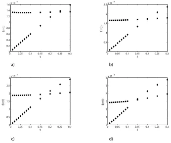
For the DNS method,Err(t )att ∼0 is the same as the initial error applied to the defined initial conditions to cre-ate the erroneous initial conditions. Since no correction has been applied, the prediction is wrong by the same amount as the error added to the initial conditions. As time increases,

(6)

262 C. A. Hier Majumder et al.: Data assimilation for plume models

6 C. A. Hier Majumder et al.: Data Assimilation for Plume Models

0 0.05 0.1 0.15 0.2 0.25 0.3 0

0.2 0.4 0.6 0.8 1 1.2 1.4 1.6x 10

−3

t

Err

(t)

0 0.05 0.1 0.15 0.2 0.25 0.3 0

0.5 1 1.5 2 2.5x 10

−3

t

Err

(t)

0 0.05 0.1 0.15 0.2 0.25 0.3 0

0.5 1 1.5 2 2.5

3x 10

−3

t

Err

(t)

0 0.05 0.1 0.15 0.2 0.25 0.3 0

1 2 3 4 5 6x 10

−3

t

Err

(t)

a) b)

c) d)

Fig. 3. Comparison between DNS and 4D-VAR at different times after an initial perturbation has been set for °U±)²³§µ³¸· ¹ . Squares

representÅy»»¡ÆÈÇÉ whenÊËÌ-Í is calculated using the DNS method. Diamonds representÅy»C»*ÆÈÇ-É whenÊ§ËÌ-Í is calculated using the 4D-VAR

method. Time,Ç, is scaled by the free-fall time. a)°U±²³yµ³¸·2¹ . b)°U±²bÎµ{³¸·¹. c)°U±²ÐÏµQ³·I¹ . d)°8±²Ñ³Òµ{³¸·2Ó.

1 2 3 4 5 6 7

4.1 4.2 4.3 4.4 4.5 4.6 4.7 4.8 x 10

−4

Iterations

Cost Function

Fig. 4. Minimization of the cost function for°8±B²Ô³µ_³¸· ¹ ,

Ç"² ·¡Õ·¡³ .

calculated from the adjoint equations. We have shown the minimization of the cost function for an example plume of

_I

, qrÖ¨

(Fig. 4). The free-fall velocity forecast time for this simulation was 0.01. The cost function is minimized by 14% over 7 iterations.

The error near

#

¥

in the 4D-VAR case is significantly lower than in the DNS case (Fig. 3). The correction is max-imal and the error is minmax-imal a very short time after

#

. In fact,«

I #%$

is almost 0. This indicates that the erroneous initial conditions have been fully corrected by the 4D-VAR

method. As time is increased, « 2

#%$

increases, and the quality of the 4D-VAR prediction degrades. At some time, known as the horizon of predictability, the 4D-VAR predic-tion is no better than the DNS predicpredic-tion to which no correc-tion was applied.

3.2.1 Effect of Rayleigh number

The horizon of predictability depends on Rayleigh number. For

Q

the horizon of predictability was 0.25 (Fig. 3a). For

9Ð

it decreased to 0.20 (Fig. 3b). For

¶

it decreased further to 0.17 (Fig. 3c), and for

§¶

it is about 0.14 (Fig. 3d). As the Rayleigh number increases, the nonlinear, inertial terms become more important, and the horizon of predictability decreases.

The quality of the 4D-VAR method is compared for dif-ferent Rayleigh numbers in Fig. 5. We defined the quality of the 4D-VAR prediction as:

× #%$

«

I #%$

/DNS

4

«

2 #%$

/4D-VAR

4

(33)

The quality increases with the Rayleigh number for small forecast times. This is due to the fact that the inertia in-creases with the Rayleigh number. As the inertia inin-creases, the plume becomes less sensitive to initial conditions. As the forecast time increases the quality decreases. This de-crease in quality, however, is less drastic for lower Rayleigh numbers. This is due to the fact that the higher the inertia

Fig. 3. Comparison between DNS and 4D-VAR at different times after an initial perturbation has been set forRa=1×106. Squares represent Err(t )whenHcalis calculated using the DNS method. Diamonds representErr(t )whenHcalis calculated using the 4D-VAR method.

Time,t, is scaled by the free-fall time. (a)Ra=1×106. (b)Ra=2×106. (c)Ra=3×106. (d)Ra=1×107.

6

C. A. Hier Majumder et al.: Data Assimilation for Plume Models

0 0.05 0.1 0.15 0.2 0.25 0.3

0 0.2 0.4 0.6 0.8 1 1.2 1.4

1.6x 10

−3

t

Err

(t)

0 0.05 0.1 0.15 0.2 0.25 0.3

0 0.5 1 1.5 2

2.5x 10

−3

t

Err

(t)

0 0.05 0.1 0.15 0.2 0.25 0.3

0 0.5 1 1.5 2 2.5

3x 10

−3

t

Err

(t)

0 0.05 0.1 0.15 0.2 0.25 0.3

0 1 2 3 4 5

6x 10

−3

t

Err

(t)

a)

b)

c)

d)

Fig. 3.

Comparison between DNS and 4D-VAR at different times after an initial perturbation has been set for

°U±)²³§µ³¸· ¹

. Squares

represent

Åy»»¡ÆÈÇÉ

when

ÊËÌ-Í

is calculated using the DNS method. Diamonds represent

Åy»C»*ÆÈÇ-É

when

Ê§ËÌ-Í

is calculated using the 4D-VAR

method. Time,

Ç

, is scaled by the free-fall time. a)

°U±²³yµ³¸·2¹

. b)

°U±²bÎµ{³¸·¹

. c)

°U±²ÐÏµQ³·I¹

. d)

°8±²Ñ³Òµ{³¸·2Ó

.

1 2 3 4 5 6 7

4.1 4.2 4.3 4.4 4.5 4.6 4.7 4.8 x 10

−4

Iterations

Cost Function

Fig. 4.

Minimization of the cost function for

°8±B²Ô³µ_³¸· ¹

,

Ç"²

·¡Õ·¡³

.

calculated from the adjoint equations. We have shown the

minimization of the cost function for an example plume of

_I

,

qrÖ¨

(Fig. 4). The free-fall velocity

forecast time for this simulation was 0.01. The cost function

is minimized by 14% over 7 iterations.

The error near

#

¥

in the 4D-VAR case is significantly

lower than in the DNS case (Fig. 3). The correction is

max-imal and the error is minmax-imal a very short time after

#

.

In fact,

«

I #%$

is almost 0. This indicates that the erroneous

initial conditions have been fully corrected by the 4D-VAR

method. As time is increased,

« 2

#%$

increases, and the

quality of the 4D-VAR prediction degrades. At some time,

known as the horizon of predictability, the 4D-VAR

predic-tion is no better than the DNS predicpredic-tion to which no

correc-tion was applied.

The horizon of predictability depends on Rayleigh number.

For

Q

the horizon of predictability was 0.25

(Fig. 3a). For

9Ð

it decreased to 0.20 (Fig. 3b).

For

¶

it decreased further to 0.17 (Fig. 3c), and

for

§¶

it is about 0.14 (Fig. 3d). As the Rayleigh

number increases, the nonlinear, inertial terms become more

important, and the horizon of predictability decreases.

The quality of the 4D-VAR method is compared for

dif-ferent Rayleigh numbers in Fig. 5. We defined the quality of

the 4D-VAR prediction as:

× #%$

«

I #%$

/

DNS

4

«

2 #%$

/

4D-VAR

4

(33)

The quality increases with the Rayleigh number for small

forecast times. This is due to the fact that the inertia

in-creases with the Rayleigh number. As the inertia inin-creases,

the plume becomes less sensitive to initial conditions. As

the forecast time increases the quality decreases. This

de-crease in quality, however, is less drastic for lower Rayleigh

numbers. This is due to the fact that the higher the inertia

Fig. 4. Minimization of the cost function forRa=1×106,t=0.01.

error begins to increase decreases withRa. ForRa=2×106,

Err(t )begins to increase after 0.20 (Fig. 3b), andErr(t ) in-creases after 0.15 forRa=3×106(Fig. 3c). ForRa=1×107, the error starts to increase immediately (Fig. 3d). The error in the direct simulation begins to increase after nonlinear, in-ertial terms become important. These terms are larger with increasing Rayleigh number. Therefore, we cannot predict as long with increasing Rayleigh number.

3.2 4D-VAR

The 4D-VAR method is used to decrease the errors due to the perturbed initial conditions. The cost function is minimized with the steepest descent method through use of its gradient calculated from the adjoint equations. We have shown the minimization of the cost function for an example plume of

Ra=1×106,P r=7 (Fig. 4). The free-fall velocity forecast time for this simulation was 0.01. The cost function is mini-mized by 14% over 7 iterations.

The error near t∼0 in the 4D-VAR case is significantly lower than in the DNS case (Fig. 3). The correction is maxi-mal and the error is minimaxi-mal a very short time aftert=0. In fact, Err(t )is almost 0. This indicates that the erroneous initial conditions have been fully corrected by the 4D-VAR method. As time is increased,Err(t )increases, and the qual-ity of the 4D-VAR prediction degrades. At some time, known as the horizon of predictability, the 4D-VAR prediction is no better than the DNS prediction to which no correction was applied.

(7)

C. A. Hier Majumder et al.: Data assimilation for plume models 263

C. A. Hier Majumder et al.: Data Assimilation for Plume Models

7

0 0.02 0.04 0.06 0.08 0.1 0.5

1 1.5 2 2.5

3 x 10

−3

t

Q(t)

Fig. 5.

Quality of the 4D-VAR prediction,

ØÆÈÇ-É

, versus free-fall

time,

Ç

. All plumes have a Prandtl number of 7. Four different

Rayleigh numbers are shown:

³µ_³·I¹

, stars;

Î+µ_³·I¹

, diamonds;

Ï§µ³¸·¹

, squares;

³yµQ³·2Ó

, circles.

in a system, the more difficult it becomes to

deterministi-cally compute its exact state through time. Therefore, for

the higher Rayleigh numbers the quality of the 4D-VAR

pre-diction decreases more rapidly in time than for the lower

Rayleigh numbers.

This means that a higher inertial system is not as likely

to be affected by small fluctuations; therefore, it has better

predictability (Lorenz, 1963). This is known as the butterfly

effect. If highly inertial system, such as the atmosphere, were

very sensitive to small perturbations, a butterfly flapping its

wings in Brazil could cause a tornado in Texas (Lorenz,

1972). The horizon of predictability decreases with

. This

means that although we can generate better predictions for

higher inertial systems, we cannot generate predictions for

as long as we can for lower inertia systems.

3.2.2 Effect of numerical resolution

In order to test whether we had used adequate numerical

resolution in our simulations, we also ran the prediction for

I

,

q©¨

in double precision (Fig. 6). Our

simula-tions were run using 32 bit single precision which gives 7

sig-nificant digits on the IBM Regatta used in this study. There is

a small decrease in the horizon of predictability from 0.25 to

0.22 indicating that it may be slightly more difficult to

pre-dict higher resolution simulations for a longer time period.

We see that there is a 12% improvement in the quality of the

prediction near

#

¥

for the doubled numerical resolution

(Fig. 7). The improvement in the quality of the prediction

due to the increased numerical resolution, however, drops as

the forecast time increases. This indicates that we can

im-prove our short term predictions by using double precision,

but that it does not tend to improve longer term predictions.

3.2.3 Effect of initial perturbation

We also tested the method with single precision using a more

random perturbation of the initial conditions (Fig. 8). This

perturbation was created by linear superposition of several

0 0.05 0.1 0.15 0.2 0.25 0.3 0

0.5 1 1.5

2 x 10

−3

t

Err(t)

Fig. 6.

Comparison of the DNS and 4D-VAR prediction for

°U±6²

³µv³¸·I¹

,

º"»²¼

with double resolution. DNS is shown with

dia-monds and 4D-VAR with squares.

0 0.02 0.04 0.06 0.08 0.1 0.6

0.8 1 1.2 1.4 1.6 x 10−3

t

Q(t)

Fig. 7.

Ø§ÆÈÇ-É

versus free-fall

time,

Ç

. The Quality is defined as the difference between the error

of the DNS and the 4D-VAR simulations. Data is shown

°U±²

³yµ{³¸·I¹

,

º"»y²¼

. Single precision is shown by squares and double

precision by diamonds.

different sinusoidal perturbations. We found that the horizon

of predictability increased for

+Ð

,

q{Y¨

from

0.25 for the original perturbation to 0.30 for the more random

perturbation (Fig. 9). For

9BÐI

,

qBY¨

, the

hori-zon of predictability increased from 0.20 to 0.25 (Fig. 10).

There is also significant improvement in the quality of the

predictions for the more random initial perturbation (Fig. 11)

versus the more regular perturbation (Fig. 5). By perturbing

different modes we do expect the response of the system to be

slightly different due to the fact that each scale has an

intrin-sic horizon of predictability (Lorenz, 1969). However, the

general conclusion still holds that the larger Rayleigh

num-ber flow has a shorter horizon of predictablity but a lower

quality prediction.

3.2.4 Effect of Prandtl number

We next ran simulations at

{

with

q kª ¨

and

qÑÙ¨

using single precision and the more regular

perturbation. For a given

, the 4D-VAR predictions are

better for a lower

q

at small forecast times (Figs. 12). This

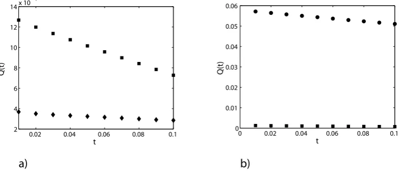
Fig. 5. Quality of the 4D-VAR prediction,Q(t ), versus free-fall

time, t. All plumes have a Prandtl number of 7. Four different Rayleigh numbers are shown: 1×106, stars; 2×106, diamonds; 3×106, squares; 1×107, circles.

C. A. Hier Majumder et al.: Data Assimilation for Plume Models

7

0 0.02 0.04 0.06 0.08 0.1 0.5

1 1.5 2 2.5

3 x 10

−3

t

Q(t)

Fig. 5.

ØÆÈÇ-É

, versus free-fall

time,

Ç

³µ_³·I¹

, stars;

Î+µ_³·I¹

, diamonds;

Ï§µ³¸·¹

, squares;

³yµQ³·2Ó

, circles.

the higher Rayleigh numbers the quality of the 4D-VAR

Rayleigh numbers.

effect. If highly inertial system, such as the atmosphere, were

. This

as long as we can for lower inertia systems.

I

,

q©¨

sig-nificant digits on the IBM Regatta used in this study. There is

prediction near

#

¥

(Fig. 7). The improvement in the quality of the prediction

3.2.3 Effect of initial perturbation

0 0.05 0.1 0.15 0.2 0.25 0.3 0

0.5 1 1.5

2 x 10

−3

t

Err(t)

Fig. 6.

°U±6²

³µv³¸·I¹

,

º"»²¼

dia-monds and 4D-VAR with squares.

0 0.02 0.04 0.06 0.08 0.1 0.6

0.8 1 1.2 1.4 1.6 x 10

−3

t

Q(t)

Fig. 7.

Ø§ÆÈÇ-É

versus free-fall

time,

Ç

°U±²

³yµ{³¸·I¹

,

º"»y²¼

of predictability increased for

+Ð

,

q{Y¨

from

9BÐI

,

qBY¨

, the

different modes we do expect the response of the system to be

quality prediction.

{

with

q kª ¨

and

qÑÙ¨

better for a lower

q

Fig. 6. Comparison of the DNS and 4D-VAR prediction for

Ra=1×106, P r=7 with double resolution. DNS is shown with diamonds and 4D-VAR with squares.

number increases, the nonlinear, inertial terms become more important, and the horizon of predictability decreases.

The quality of the 4D-VAR method is compared for dif-ferent Rayleigh numbers in Fig. 5. We defined the quality of the 4D-VAR prediction as:

Q(t )=Err(t )[DNS] −Err(t )[4D-VAR]. (33) The quality increases with the Rayleigh number for small forecast times. This is due to the fact that the inertia in-creases with the Rayleigh number. As the inertia inin-creases, the plume becomes less sensitive to initial conditions. As the forecast time increases, the quality decreases. This de-crease in quality, however, is less drastic for lower Rayleigh

C. A. Hier Majumder et al.: Data Assimilation for Plume Models

7

0 0.02 0.04 0.06 0.08 0.1 0.5

1 1.5 2 2.5

3 x 10

−3

t

Q(t)

Fig. 5.

ØÆÈÇ-É

, versus free-fall

time,

Ç

³µ_³·I¹

, stars;

Î+µ_³·I¹

, diamonds;

Ï§µ³¸·¹

, squares;

³yµQ³·2Ó

, circles.

the higher Rayleigh numbers the quality of the 4D-VAR

Rayleigh numbers.

effect. If highly inertial system, such as the atmosphere, were

. This

as long as we can for lower inertia systems.

I

,

q©¨

sig-nificant digits on the IBM Regatta used in this study. There is

prediction near

#

¥

(Fig. 7). The improvement in the quality of the prediction

3.2.3 Effect of initial perturbation

0 0.05 0.1 0.15 0.2 0.25 0.3 0

0.5 1 1.5

2 x 10

−3

t

Err(t)

Fig. 6.

°U±6²

³µv³¸·I¹

,

º"»²¼

dia-monds and 4D-VAR with squares.

0 0.02 0.04 0.06 0.08 0.1 0.6

0.8 1 1.2 1.4 1.6 x 10

−3

t

Q(t)

Fig. 7.

Ø§ÆÈÇ-É

versus free-fall

time,

Ç

°U±²

³yµ{³¸·I¹

,

º"»y²¼

of predictability increased for

+Ð

,

q{Y¨

from

9BÐI

,

qBY¨

, the

different modes we do expect the response of the system to be

quality prediction.

{

with

q

kª¨

and

qÑÙ¨

better for a lower

q

Fig. 7. Quality of the 4D-VAR prediction, Q(t ) versus free-fall

time,t. The Quality is defined as the difference between the error of the DNS and the 4D-VAR simulations. Data is shownRa=1×106, P r=7. Single precision is shown by squares and double precision by diamonds.

8 C. A. Hier Majumder et al.: Data Assimilation for Plume Models

Fig. 8.A more random perturbation on the initial temperature con-ditions for°U±B²O³µ_³·

¹2Ú

º"»²r¼ . The initial conditions are the

same as shown in Fig. 2a. Scale for the nondimensional temperature ranges from 0 for black to 0.06 for white.

0 0.1 0.2 0.3 0.4 0.5 0 0.5 1 1.5 2 2.5 3 3.5

4 x 10−3

t

Err(t)

Fig. 9. Comparision of DNS and 4D-VAR prediction for a more random initial perturbation of a plume with°U±²³mµe³· ¹,º"»"²b¼ .

DNS prediction is shown by diamonds and 4D-VAR prediction by squares.

0 0.05 0.1 0.15 0.2 0.25 0.3 0 0.5 1 1.5 2 2.5 3 3.5

4 x 10

−3

t

Err(t)

Fig. 10. Comparision of DNS and 4D-VAR prediction for a more random initial perturbation of a plume with°U±²bÎ]µe³·2¹,º"»"²b¼ .

DNS prediction is shown by diamonds and 4D-VAR prediction by squares.

0 0.05 0.1 0.15 0.2 0.25 0.3 0 0.5 1 1.5 2 2.5

3 x 10−3

t

Q(t)

Fig. 11. Comparision of quality of 4D-VAR prediction for plumes of different Rayleigh number with a more random initial pertur-bation °U±Û²Ü³µ³¸· ¹ , º"»r²Ý¼ is shown by diamonds, and

°U±²Îµ³¸· ¹ ,º"»"²¼ is shown by squares.

is due to the fact that inertia strengthens as q

decreases. We were only able to study plumes with Prandtl numbers up to 70 in this study. Previous studies of plume behavior with Prandtl numbers up to 20,000 (Hier Majumder et al., 2004) have shown that there are still significant differences between finite and infinite Prandtl plumes even at these Rayleigh num-bers. It would be interesting conduct similar studies on the predictability of high and infinite Prandtl number plumes. Although our method can theoretically handle higher Prandtl numbers, it would be necessary, however, to deal with the increasing stiffness of the finite Prandtl number convection equations along with the resulting large grid sizes. For ex-ample, plumes with Prandtl numbers on the order of (Þ

at Rayleigh numbers of

would require grid sizes of 512 x 1536 (Hier Majumder et al., 2004). Since each step of the forward solution is needed to solve the adjoint solution, the major computational expense of the adjoint method is the memory resources needed for storage of the forward solu-tion (Daescu et al., 2003). Methods that have been devel-oped for using the adjoint method with the stiff equations of atmospheric chemistry could prove useful for predictability studies of the large Prandtl numbers plumes (Elbern et al., 1997; Daescu et al., 2000; Sandu et al., 2003; Daescu et al., 2003).

4 Conclusions

We found that the 4D-VAR method is successful at correct-ing simulations that have erroneous initial conditions for fi-nite Prandtl plumes. This technique can increase the ability to model plume phenomena for which observations, such as laboratory and seismic data, are available, but where the ex-act initial conditions are not well known. The 4D-VAR cor-rection only works for a limited time, however. The time limit for the prediction is known as the predictability time.

We saw that as the inertia of the system increases with in-creasing Rayleigh number, the predictability time decreases. However, we also saw that we can generate better 4D-VAR

Fig. 8. A more random perturbation on the initial temperature con-ditions forRa=1×106, P r=7. The initial conditions are the same as shown in Fig. 2a. Scale for the nondimensional temperature ranges from 0 for black to 0.06 for white.

numbers. This is due to the fact that the higher the inertia in a system, the more difficult it becomes to deterministi-cally compute its exact state through time. Therefore, for the higher Rayleigh numbers the quality of the 4D-VAR pre-diction decreases more rapidly in time than for the lower Rayleigh numbers.

(8)

264 C. A. Hier Majumder et al.: Data assimilation for plume models

8

C. A. Hier Majumder et al.: Data Assimilation for Plume Models

Fig. 8.

A more random perturbation on the initial temperature

con-ditions for

°U±B²O³µ_³·

¹2Ú

º"»²r¼

. The initial conditions are the

same as shown in Fig. 2a. Scale for the nondimensional temperature

ranges from 0 for black to 0.06 for white.

0 0.1 0.2 0.3 0.4 0.5

0 0.5 1 1.5 2 2.5 3 3.5

4 x 10

−3

t

Err(t)

Fig. 9.

Comparision of DNS and 4D-VAR prediction for a more

random initial perturbation of a plume with

°U±²³mµe³· ¹

,

º"»"²b¼

.

DNS prediction is shown by diamonds and 4D-VAR prediction by

squares.

0 0.05 0.1 0.15 0.2 0.25 0.3 0

0.5 1 1.5 2 2.5 3 3.5

4 x 10

−3

t

Err(t)

Fig. 10.

random initial perturbation of a plume with

°U±²bÎ]µe³·2¹

,

º"»"²b¼

.

squares.

0 0.05 0.1 0.15 0.2 0.25 0.3 0

0.5 1 1.5 2 2.5

3 x 10

−3

t

Q(t)

Fig. 11.

Comparision of quality of 4D-VAR prediction for plumes

of different Rayleigh number with a more random initial

pertur-bation

°U±Û²Ü³µ³¸· ¹

,

º"»r²Ý¼

is shown by diamonds, and

°U±²Îµ³¸· ¹

,

º"»"²¼

is shown by squares.

is due to the fact that inertia strengthens as

q

decreases.

We were only able to study plumes with Prandtl numbers up

to 70 in this study. Previous studies of plume behavior with

Prandtl numbers up to 20,000 (Hier Majumder et al., 2004)

have shown that there are still significant differences between

finite and infinite Prandtl plumes even at these Rayleigh

num-bers. It would be interesting conduct similar studies on the

predictability of high and infinite Prandtl number plumes.

Although our method can theoretically handle higher Prandtl

numbers, it would be necessary, however, to deal with the

increasing stiffness of the finite Prandtl number convection

equations along with the resulting large grid sizes. For

ex-ample, plumes with Prandtl numbers on the order of

(Þ

at

Rayleigh numbers of

would require grid sizes of 512 x

1536 (Hier Majumder et al., 2004). Since each step of the

forward solution is needed to solve the adjoint solution, the

major computational expense of the adjoint method is the

memory resources needed for storage of the forward

solu-tion (Daescu et al., 2003). Methods that have been

devel-oped for using the adjoint method with the stiff equations of

atmospheric chemistry could prove useful for predictability

studies of the large Prandtl numbers plumes (Elbern et al.,

1997; Daescu et al., 2000; Sandu et al., 2003; Daescu et al.,

2003).

4 Conclusions

We found that the 4D-VAR method is successful at

correct-ing simulations that have erroneous initial conditions for

fi-nite Prandtl plumes. This technique can increase the ability

to model plume phenomena for which observations, such as

laboratory and seismic data, are available, but where the

ex-act initial conditions are not well known. The 4D-VAR

cor-rection only works for a limited time, however. The time

limit for the prediction is known as the predictability time.

We saw that as the inertia of the system increases with

in-creasing Rayleigh number, the predictability time decreases.

However, we also saw that we can generate better 4D-VAR

Fig. 9. Comparision of DNS and 4D-VAR prediction for a more random initial perturbation of a plume withRa=1×106, P r=7. DNS prediction is shown by diamonds and 4D-VAR prediction by squares.

8

C. A. Hier Majumder et al.: Data Assimilation for Plume Models

Fig. 8.

A more random perturbation on the initial temperature

con-ditions for

°U±B²O³µ_³·

¹2Ú

º"»²r¼

0 0.1 0.2 0.3 0.4 0.5

0 0.5 1 1.5 2 2.5 3 3.5

4 x 10

−3

t

Err(t)

Fig. 9.

°U±²³mµe³·

¹

,

º"»"²b¼

.

DNS prediction is shown by diamonds and 4D-VAR prediction by

squares.

0 0.05 0.1 0.15 0.2 0.25 0.3 0

0.5 1 1.5 2 2.5 3 3.5

4 x 10

−3

t

Err(t)

Fig. 10.

°U±²bÎ]µe³·2¹

,

º"»"²b¼

.

squares.

0 0.05 0.1 0.15 0.2 0.25 0.3 0

0.5 1 1.5 2 2.5

3 x 10

−3

t

Q(t)

Fig. 11.

Comparision of quality of 4D-VAR prediction for plumes

of different Rayleigh number with a more random initial

pertur-bation

°U±Û²Ü³µ³¸·

¹

,

º"»r²Ý¼

is shown by diamonds, and

°U±²Îµ³¸· ¹

,

º"»"²¼

is shown by squares.

is due to the fact that inertia strengthens as

q

decreases.

We were only able to study plumes with Prandtl numbers up

to 70 in this study. Previous studies of plume behavior with

Prandtl numbers up to 20,000 (Hier Majumder et al., 2004)

have shown that there are still significant differences between

finite and infinite Prandtl plumes even at these Rayleigh

num-bers. It would be interesting conduct similar studies on the

predictability of high and infinite Prandtl number plumes.

Although our method can theoretically handle higher Prandtl

numbers, it would be necessary, however, to deal with the

increasing stiffness of the finite Prandtl number convection

equations along with the resulting large grid sizes. For

ex-ample, plumes with Prandtl numbers on the order of

(Þ

at

Rayleigh numbers of

would require grid sizes of 512 x

1536 (Hier Majumder et al., 2004). Since each step of the

forward solution is needed to solve the adjoint solution, the

major computational expense of the adjoint method is the

memory resources needed for storage of the forward

solu-tion (Daescu et al., 2003). Methods that have been

devel-oped for using the adjoint method with the stiff equations of

atmospheric chemistry could prove useful for predictability

studies of the large Prandtl numbers plumes (Elbern et al.,

1997; Daescu et al., 2000; Sandu et al., 2003; Daescu et al.,

2003).

4 Conclusions

We found that the 4D-VAR method is successful at

correct-ing simulations that have erroneous initial conditions for

fi-nite Prandtl plumes. This technique can increase the ability

to model plume phenomena for which observations, such as

laboratory and seismic data, are available, but where the

ex-act initial conditions are not well known. The 4D-VAR

cor-rection only works for a limited time, however. The time

limit for the prediction is known as the predictability time.

We saw that as the inertia of the system increases with

in-creasing Rayleigh number, the predictability time decreases.

However, we also saw that we can generate better 4D-VAR

Fig. 10. Comparision of DNS and 4D-VAR prediction for a more random initial perturbation of a plume withRa=2×106, P r=7. DNS prediction is shown by diamonds and 4D-VAR prediction by squares.

(Lorenz, 1972). Although the quality of the prediction im-proves withRa, the horizon of predictability decreases with

Ra. This means that although we can generate better tions for higher inertial systems, we cannot generate predic-tions for as long as we can for lower inertia systems. 3.2.2 Effect of numerical resolution

In order to test whether we used adequate numerical res-olution in our simulations, we also ran the prediction for

Ra=106, P r=7 in double precision (Fig. 6). Our simula-tions were run using 32 bit single precision which gives 7

sig-8

C. A. Hier Majumder et al.: Data Assimilation for Plume Models

Fig. 8.

A more random perturbation on the initial temperature

con-ditions for

°U±B²O³µ_³· ¹2Ú º"»²r¼

0 0.1 0.2 0.3 0.4 0.5

0 0.5 1 1.5 2 2.5 3 3.5

4 x 10

−3

t

Err(t)

Fig. 9.

random initial perturbation of a plume with

°U±²³mµe³·

¹

,

º"»"²b¼

.

squares.

0 0.05 0.1 0.15 0.2 0.25 0.3 0

0.5 1 1.5 2 2.5 3 3.5

4 x 10

−3

t

Err(t)

Fig. 10.

random initial perturbati