SRef-ID: 1607-7946/npg/2005-12-149 European Geosciences Union
© 2005 Author(s). This work is licensed under a Creative Commons License.
Nonlinear Processes
in Geophysics
Developing a dynamically based assimilation method for targeted
and standard observations
F. Uboldi1, A. Trevisan2, and A. Carrassi3
1LEGOS/SHOM, Toulouse, France 2CNR-ISAC, Bologna, Italy
3Dipartimento di Fisica – Universit`a di Ferrara, Italy
Received: 31 August 2004 – Revised: 22 December 2004 – Accepted: 7 January 2005 – Published: 28 January 2005 Part of Special Issue “Quantifying predictability”
Abstract. In a recent study, a new method for assimilat-ing observations has been proposed and applied to a small size nonlinear model. The assimilation is obtained by con-fining the analysis increment in the unstable subspace of the Observation-Analysis-Forecast (OAF) cycle system, in order to systematically eliminate the dynamically unstable com-ponents, present in the forecast error, which are responsi-ble for error growth. Based on the same ideas, applications to more complex models and different, standard and adap-tive, observation networks are in progress. Observing Sys-tem Simulation Experiments (OSSE), performed with an at-mospheric quasi-geostrophic model, with a restricted “land” area where vertical profiles are systematically observed, and a wider “ocean” area where a single supplementary observa-tion is taken at each analysis time, are reviewed. The adaptive observation is assimilated either with the proposed method or, for comparison, with a 3-D VAR scheme. The perfor-mance of the dynamic assimilation is very good: a reduc-tion of the error of almost an order of magnitude is obtained in the data void region. The same method is applied to a primitive equation ocean model, where “satellite altimetry” observations are assimilated. In this standard observational configuration, preliminary results show a less spectacular but significant improvement obtained by the introduction of the dynamical assimilation.
1 Introduction
Data assimilation in meteorology and oceanography deals with high-dimensional chaotic systems. In such systems, er-rors which are present in the initial condition grow in time, due to instability. Other errors are of course introduced along
Correspondence to: F. Uboldi
the Observation-Analysis-Forecast (OAF) cycle. Model er-rors of various origin are introduced along the forecasting integration, and observation errors (including errors in the observation operator) are introduced at analysis time. Any-how all these errors eventually increase or decrease depend-ing on the action of the dynamical instabilities of the system. A relevant point, then, is observability (Ghil, 1997): how many perfect observations, under perfect model conditions, are necessary to exactly determine the state of the system? The answer depends on the number of independent unstable directions.
The OAF cycle is seen as a dynamical system, subject to observational forcing. Its perturbations (tangent linear) dy-namics is, for analysis states:
δxak+1=(I−KH)Mδxak, (1) where K is the assimilation matrix (Kalman gain), H is the linearized observation operator, M is the tangent linear model and I is the identity matrix. It is the stability of such a system that characterizes the tendency of the sequence of analysis states (or the sequence of forecast states at assimi-lation times) to approach or depart from the trajectory of the real system, at least when the two trajectories are sufficiently close to each other. As a consequence, what is of concern is the dimension of the unstable subspace of such a forced system.
Generally, but depending on the specific implementation choices of each assimilation scheme, the forcing due to the assimilation of observations results in a reduction of the di-mension of the unstable subspace. As a consequence, the order of the problem is reduced, and only few supplemen-tary observations are in some cases sufficient to control the system. The method we propose is intended to focus on this mechanism of order reduction.
150 F. Uboldi et al.: A dynamically based assimilation method configurations. Its first application to a small size nonlinear
model (Lorenz and Emanuel, 1998), together with a mathe-matical description of the method, can be found in Trevisan and Uboldi (2004), hereafter TU. Results obtained with the proposed assimilation scheme were compared with an exper-iment in which an Optimal Interpolation type of analysis was used to assimilate the adaptively located observations. Er-rors, both in the analysis state and in forecasts based on it, were significantly and systematically reduced. A strong in-crease in the stability of the OAF system was achieved, mea-sured by a strong decrease of the dominant exponent; this is a further indication of the successful control of instabili-ties. Readers are referred to the paper for further details. A brief description of the method and its implementation can be found in Sect. 2 of the present work. Results obtained with targeted observations in the context of a quasi-geostrophic atmospheric model are described in Sect. 3. Presently, work is being devoted to extending the proposed method to a prim-itive equation ocean model, and some preliminary results with a standard (i.e. non-targeted) observation network are described in Sect. 4.
2 Assimilation within the unstable subspace
In order to confine the assimilation in the unstable subspace, a reliable estimate of the most unstable directions has to be made available at each assimilation time. In principle, the unstable subspace should be formed by the Lyapunov vec-tors with corresponding positive exponents. In practice, these vectors are estimated by breeding on the data assimilation cy-cle, as extensively discussed in Carrassi et al. (under review, 20051), hereafter CTU. The breeding technique introduced by Toth and Kalnay (1997) has been modified to estimate the unstable vectors of the forced OAF system. To estimate the unstable subspace of the OAF system, observations are assimilated in each perturbed trajectory as it is done in the control trajectory. Because the unstable vectors are only ap-proximate estimates of the forecast error, a further step is necessary in order to make them better proxies of the true forecast error structure. At analysis time, a regionalization procedure is used in order to select and isolate, from each bred vector of the current set, one or more “structures”, iden-tified as local maxima or minima. This is obtained by means of a Gaussian-shaped modulating function, centered in each maximum or minimum, and applied to the bred vector by point-by-point multiplication. The N vectors obtained in this way have the local structure of one of the current bred vec-tors and are stored in the N columns of a matrix, E, whose number of rows, I, is the state dimension. More details on the regionalization procedure are given, with regard to the
1Carrassi, A., Trevisan, A., and Uboldi, F.: Deterministic Data
Assimilation and Targeting by Breeding on the Data Assimilation System, J. of Atmos. Sci., under review, 2005.
specific implementations, in Sects. 3 and 4. The matrix E is used to estimate the forecast error covariance matrix:
Pf =E0ET (2)
or, in other words, the analysis increment is confined in the estimated unstable subspace:
xa=xf +Ea. (3)
Here the (N,N) matrix0represents the forecast error covari-ance in the subspace spanned by the columns of E, while the vector of coefficients a is the control variable, i.e. the analy-sis increment in that subspace. The mathematical expression of the analysis solution has then the same form as that of En-semble Kalman Filters (Evensen, 2003), hereafter EnKF, the difference being in how E is built:
xa =xf +E0(HE)Th(HE)0(HE)T+Ri −1
·yo−Hxf (4)
or, equivalently, :
xa =xf +Eh0−1+(HE)T R−1(HE)i
−1
(HE)T
·R−1yo−Hxf, (5)
where the vector yo contains the observations, R is the ob-servation error covariance matrix and H is the (possibly non-linear) observation operator, whose Jacobian is H.
In the case of targeted observations, one observation is lo-cated in the proximity of the maximum component of each unstable vector, so that the number, M, of observations must be at least equal to N.
In the case of standard observations, that is to say a fixed observation network, the important question is the follow-ing. If we are able to provide a correct estimate of the un-stable structures, are these structures located in geographical regions where routine observations are available? If they are, they can be effectively used. Even if, occasionally, the unsta-ble structures go undetected, they might migrate into a more densely observed region, then be detected at a later assimi-lation time, so that our ability to control the solution is not compromised. In both cases, there are two important points: how large is the number of the unstable structures, and how fast they grow compared to the frequency with which we are able to observe and eliminate them.
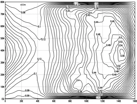
Fig. 1. QG model. Data-dense “land” on longitudes 0-50E. One
adaptive observation is located in the data-void “ocean”, longitudes 50E-160E. Level and time averaged RMS analysis error, when the adaptive observation is assimilated with 3-D VAR.
3 Application to a Quasi-Geostrophic atmospheric model
The method has been applied to an atmospheric quasi-geostrophic model (Rotunno and Bao, 1996; Morss, 1999). Results presented in this section are included in CTU, where an extended theoretical discussion, complete results with per-fect and noisy observations and a detailed stability analy-sis can be found. The domain is a periodic channel, with 64 longitude, 33 latitude gridpoints (16 000 km×8000 km). Potential vorticity is defined on 5 inner vertical levels, and potential temperature is defined at top and bottom bound-aries. Observations are assimilated every 12 h. Here we chose perfect model conditions, and perfect observations are assimilated: a long reference model trajectory represents the “true” state evolution, from which observations are taken.
A “land” area is defined, in the western third of the domain (longitudinal grid-points 1–20), where fixed observations are located at each grid-point and assimilated with the 3-D VAR scheme described in Morss (1999). The remaining part of the domain is a wider “ocean” area (longitudes 21–64), on the east in the figures. The fixed observations consist of vertical profiles, measuring temperature and the two components of the horizontal wind. In the wide ocean area, at each analysis time, just one observation is adaptively located (targeted) in the maximum of one unstable vector, bred for 10 days, so that, here,M=N=1 .
For the reasons discussed at the end of the previous sec-tion, the “current” bred vector, that is used in the assimila-tion, is discarded afterwards, and a new random perturbation starts its breeding cycle. A new bred vector will be ready at the next analysis time (+12 h), because it has been introduced (9 days and 12 h) earlier.
Two different experiments, of 2 years simulated time, are performed, with the same trajectory representing the truth.
Fig. 2. Same as in Fig. 1, when the adaptive observation is
assimi-lated with the proposed method.
The adaptive observation is assimilated with the 3-D VAR scheme in experiment (1), and with the proposed method in experiment (2), while 3-D VAR is used in both experiments for assimilating the fixed observations over land. Moreover, in experiment (1) the adaptive observation consists of a complete vertical profile (temperature and wind components on 7 levels), while in experiment (2) the adaptive observation consists of a single scalar temperature observation. In both cases the adaptive observation is located in the maximum of the “current” perturbation, so the main difference is in how the adaptive observation is assimilated.
TU noted, in the small model context, the necessity of regionalizing the correction made by using the unstable structure. As explained there, this is basically due to the possible occurrence of regions oppositely correlated, with re-spect to the main maximum, in the forecast error and in the perturbation used in the assimilation. The forecast error is the superposition of different modes, that can show separate maxima and minima having different amplitude, occasion-ally opposite sign, with respect to those of the bred vector. So, while the assimilation of the observation effectively elim-inates the main error structure, the presence of a secondary one could lead to a correction with the wrong sign. The re-gionalization is obtained here in the same way as in TU, by means of a modulating function, point-by-point multiplying the “assimilating” perturbation. The choice is a Gaussian function, with (e−1) decay scale of 2500 km, much larger than the typical scale of single structures.
152 F. Uboldi et al.: A dynamically based assimilation method
0 100 200 300 400 500 600 700 0
0.1 0.2 0.3 0.4 0.5 0.6 0.7 0.8 0.9 1
Days
Analysis Error
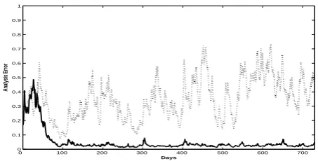
Fig. 3. QG model. RMS analysis error versus time, measured by
total enstrophy and normalized by natural variability. 3-D VAR: dotted line. Proposed method: continuous line.
0 0.2 0.4 0.6 0.8 1 1.2 1.4
0 360 720 1080 1440 1800 2160 days
Fig. 4. Ocean model. Forecast (continuous line) and Analysis
(dot-ted line) total energy error (normalized to natural variability) for the standard Cooper-Haines assimilation scheme, starting from a ran-domly chosen initial “Forecast” state.
Figure 3 shows the analysis error, plotted versus time, for comparison of the results obtained by assimilating the adap-tive observation with 3-D VAR (dotted line) or with the pro-posed method (continuous line).
A detailed stability analysis can be found in CTU. Syn-thetically, the 3-D VAR experiment shows a positive average growth rate, indicating instability, while with the proposed method a negative growth rate, that is to say stabilization, has been obtained. The value of the average growth rate de-pends essentially on how the unstable structures develop in the wide ocean area and on how successfully they are con-trolled by the assimilation of the adaptive observations.
4 Preliminary results with a primitive equation ocean model
The method is currently being applied to a primitive equation ocean model, the isopycnal model MICOM (Bleck, 1978; Baraille and Filatoff, 1995), in a simplified configuration: a flat bottom basin, with a 180×140 horizontal grid and 4 lay-ers, with constant surface wind forcing. The typical dynamic situation is that of a double gyre, cyclonic in the northern half of the domain, anticyclonic in the southern half, with an eastward stream detaching from the western boundary and a
0 0.2 0.4 0.6 0.8 1 1.2 1.4
0 360 720 1080 1440 1800 2160 days
Fig. 5. Same as Fig. 4, but starting from an initial Forecast state
whose error has been rescaled to 0.1 of variability.
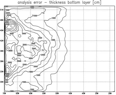
Fig. 6. Ocean model, standard Cooper-Haines analysis. RMS error
fields averaged over 6 years: forecast error on thickness of bottom layer.
Fig. 7. Same as Fig. 6, analysis error.
Error structures which are well corrected by the CH scheme are characterized by an error in the vertical position of the density gradient, which can be reduced by modify-ing the thicknesses of the first and bottom layers only, so that they compensate each other and don’t change the bottom pressure. On the other hand, error structures are sometimes compensated internally: there exist surface structures that are not evident in the bottom layer, and bottom structures that are not evident at the surface. Figures 6 and 7 show the 6 years averaged forecast and analysis root-mean-square error on the thickness of the deepest layer 4 (that is to say the elevation from the flat bottom of the interface between layers 3 and 4). It is possible to see that errors present in the forecast are associated with the eastward stream, which usually detaches from the western boundary between latitudes 39 N and 42 N, while other errors are associated with interactions between the western boundary and the northern cyclonic and southern anticyclonic gyres. The CH corrections are mostly located in the stream region, but other errors remain, and at least part of them affect the bottom pressure, as it can be seen in Fig. 8. Moreover, the analysis error is even larger than the forecast error in the northwestern part of the domain. These results support the need for more realistic and flow-dependent verti-cal covariances in the assimilation of surface height observa-tions.
Work is at present devoted to implement the proposed as-similation method with this ocean model and observation network. The idea is to exploit the information given by the standard observation network described above. As discussed in Sect. 2, ideally the column vectors of the matrix E are the Lyapunov vectors of the data assimilation system with cor-responding positive exponents. To the authors’ knowledge there is no practically convenient way to estimate the individ-ual, generally non-orthogonal, Lyapunov vectors (Trevisan and Pancotti, 1998). In the absence of orthogonalization, the bred perturbations are likely to display similar structures. In
Fig. 8. Same as Figs. 6 and 7, bottom pressure error.
the following we describe the procedure we adopted to iden-tify those structures that are most representative of the unsta-ble vectors and of the forecast error.
A CH analysis scheme starting from a climatological ini-tial forecast state reaches in a year its typical error values, between 0.3 and 0.4 of natural variability. At this point (day 360), perturbations are initially introduced and bred for 2 months, during which the only assimilation running is still CH. This is a first result: a breeding time of about 60 days, which for the ocean is not a long time, is sufficient to produce perturbations whose structures are correlated with structures present in the forecast error. At each assimilation time (ev-ery 10 days) a set of 6 independent perturbations are intro-duced. Initial perturbations are built randomly as differences from model states. At the end of the initial 2 months period (day 420), 36 perturbed states are available. At day 420, the new assimilation system begins to act. Each of the 6 “cur-rent” perturbations, the oldest set, is searched for local max-ima and minmax-ima structures, starting from the largest (in ab-solute value).
In the current implementation, four steps are taken at analysis time: regionalization, selection, assimilation and re-fresh.
– Regionalization
154 F. Uboldi et al.: A dynamically based assimilation method an excessive deformation of the structure. Anyhow the
Gaussian must not be too wide, because otherwise it may include unwanted secondary structures. By means of this procedure, a (variable) number of “structures” are extracted from the “current” perturbations. A dif-ferent “localization” technique, which appears system-atic, but also computationally expensive (and, perhaps, still risky in areas where unstable structures are only marginally detected by observations) has been proposed by Ott et al. (2004).
– Selection
A smaller number of these structures is then selected for use in the assimilation, by comparing each of them with the local structure of the innovation (difference between the observations and the forecast estimate) and retain-ing only those that show a regional correlation larger than 0.8 in absolute value. The correlation is computed by means of a euclidean scalar product between the sea surface elevation component of the structure, He, and the innovation, regionalized with the same Gaussian. The information content of the innovation is rich (in the horizontal directions) in this case. In a more realistic context this comparison could be made with, for exam-ple, the portion of satellite tracks which cross the struc-ture. Or, in the case of vertical profiles, by comparing the vertical structure of the innovation with that of the structure. The number of selected structures is usually small, not greater than 8: this is consistent with previ-ous results, obtained with the QG model in Sect. 3 and with the small model in TU. It is also consistent with recent studies which show a local low dimensionality of ensemble structures (Patil et al., 2001; Oczkowski et al., 2005).
The regionalization and selection procedures are per-formed by considering the surface elevation only, while the modulated perturbations enter the assimilation as full tridimensional fields of state variables.
– Assimilation
The selected structures are stored in the columns of the matrix E and used in the assimilation. From Eq. 5, by assuming R=σo2I and neglecting the resulting term
σo20−1(perfect observations), the analysis increment is
obtained as:
xa=xf +Eh(HE)T(HE)
i−1
(HE)T
·yo−Hxf. (6)
Is is interesting to examine the case of many observa-tions used with a single structure,M>N=1. Then the matrix E has one column only, E=e, and:
xa=xf +e(He)T y
o−H xf
(He)T(He)
. (7)
This solution minimizes (in this case Hxa −
Hxf=H xa−xf
exactly) the expression:
H xa−
yoT
H xa−
yo=
MI N (8) subject to the strong constraint (compare with Eq. 3):
xa=xf +ea . (9)
Here it can be seen how the analysis increment, con-strained by Eq. 9 in the direction of the vector e, has the amplitude that best-fits the observations.
The application of the method is intended here to ac-count for that part of the forecast error belonging to the (estimated) unstable subspace, and that is detected by means of the – supposed unchangeable – standard ob-servation network. A part of the forecast error is how-ever present that is outside the estimated unstable sub-space. For this reason the proposed method is used here in combination with the standard analysis. The anal-ysis obtained by means of the described procedure is then used as a background field for a standard CH anal-ysis. In this case the standard CH analysis is intended to be augmented rather than replaced by the proposed method.
– Refresh
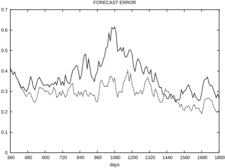
0 0.1 0.2 0.3 0.4 0.5 0.6 0.7
360 480 600 720 840 960 1080 1200 1320 1440 1560 1680 1800 days
FORECAST ERROR
Fig. 9. Ocean model. Total energy forecast error (normalized to
nat-ural variability) for the standard CH assimilation alone (continuous line) and for the proposed “sequential” method (dotted line).
extracted and used in the assimilation, still carry use-ful information. For example, some other structures are present in deeper layers, besides those evident at the sur-face at analysis time: such structures may emerge (and hopefully be detected) later on. So, the following proce-dure has been implemented as a trade-off between keep-ing or discardkeep-ing the bred vectors altogether. After the assimilation, one (at turns) of the “current” bred vec-tors (from which the estimated unstable structures have been extracted) is added to all the other 5 vectors of the same set. One new random perturbation is inserted at its place. The new set of 6 vectors start then to undergo a new 60-day breeding cycle.
The purpose of these experiments is to show how, in the presence of a standard, fixed observation network, our method can be used to eliminate, by means of the assimila-tion, those unstable structures that are present in the forecast error and that can be detected from the observations avail-able in specific geographical regions. In the present case this means that we can only detect those unstable structures that have an important component in the sea surface elevation. There exist unstable structures, confined in deeper layers, that do not appear in the sea surface elevation field. As long as they don’t emerge at the surface, those structure cannot be detected by the fixed observation network used here, but they could be detected by means of adaptive observations, as it is the case for the QG model in Sect. 3. We have per-formed experiments in which a variable number N of struc-tures are extracted (by regionalization), selected, stored in the
N columns of the matrix E and assimilated by means of Eq. 6.
Results of these experiments (not presented here) show some improvements, that are not, anyhow, systematic. In particu-lar, the sudden growth that appears at about day 980 in the standard assimilation forecast and analysis errors of Figs. 9 and 10 (continuous line), is not satisfactorily controlled. This depends on several factors. One of them is the presence of in-stabilities in deeper layers that can only be detected by means
0 0.1 0.2 0.3 0.4 0.5 0.6 0.7
360 480 600 720 840 960 1080 1200 1320 1440 1560 1680 1800 days
ANALYSIS ERROR
Fig. 10. Same as Fig. 9, analysis error.
of adaptive observations. Another problem that has been di-agnosed is the following. The same local structure (or struc-tures with very similar feastruc-tures) appears in two bred vectors of the current set. If the two structures are considered as independent vectors, and both used in the assimilation, the analysis increment can be important in the direction of the difference of the two fields, that, after the regionalization, is not guaranteed to be a well structured unstable direction. This problem was only partially overcome in these experi-ments, by computing the (surface elevation) correlation be-tween all couples of selected structures, and excluding one of the two if the correlation is larger than 0.99. A simple way of accounting for this problem is obtained by using Eq. 7 with each structure in a sequence, rather than Eq. 6 with all the selected structures together. The sequence concerns the regionalization, selection and assimilation steps, on the con-trol and on all perturbed states. In this way when a structure is eliminated, it is eliminated from all bred vectors and is as-similated only once. The two assimilations differ in regions where structures are overlapping. The results obtained with this sequential procedure are shown (dotted line) in Fig. 9 (forecast error) and Fig. 10 (analysis error), in comparison with the standard CH assimilation (continuous line). It can be seen that in this way the error peak starting at day 980 is well controlled, as are other secondary peaks. We inspected the characteristics of the flow during the period, lasting ap-proximately six months, when the standard assimilation is unable to control the instabilities and the errors become very large. It appears that, during this period, the meanders of the current are very pronounced and the local structures in the bred vectors are all concentrated and persist longer than usual in the region where the current sharply bends on itself. Such type of a flow appears to be particularly unpredictable and, when this happens, the need to use the dynamically con-sistent assimilation becomes imperative.
156 F. Uboldi et al.: A dynamically based assimilation method subsequent error growth. We expect that the use of
adap-tive observations with this ocean system, by analogy with QG model experiments, will improve the performance of the assimilation.
5 Conclusions
The experiments described here are based on the new method proposed in TU, which provides a dynamically consistent analysis state by confining the analysis increment in the un-stable subspace of the assimilation system itself. In this way instabilities which are otherwise responsible for error growth are eliminated. With this method it is possible to ex-ploit the observational forcing in the control of instabilities and consequent reduction of the dimension of the assimila-tion system unstable subspace. Only few unstable structures need to be eliminated at each assimilation time: this can be achieved by means of few adaptively located observations, or exploiting the existing fixed observation networks.
In a quasi-geostrophic atmospheric model, a significant er-ror reduction was obtained compared with a 3-D VAR assim-ilation, when the estimate of the unstable subspace is used to locate and assimilate adaptive observations
Experiments with a primitive equation ocean model showed that advantage can be taken from a fixed observation network to detect and eliminate at least some of the unstable structures.
Future developments concern the combination of adaptive and standard noisy observations, the assimilation of observa-tions distributed in time, and the approach to the assimilation of real data.
Acknowledgements. We thank R. Morss and M. Corazza for the
QG model and its 3-D VAR system, and R. Baraille for the SHOM version of MICOM.
Part of this work has been supported by the projects EPSHOM-UBO: 00.87.118.00.470.29.25 and CA2003/03/CMO.
Edited by: S. Vannitsem Reviewed by: two referees
References
Baraille, R. and Filatoff, N.: Mod`ele shallow-water multi-couches isopycnal de Miami, Tech. rep., Rapport d’´etude SHOM N.003/95, Toulouse, France, 1995.
Bleck, R.: Simulation of Coastal Upwelling Frontogenesis with an Isopycnic Coordinate Model, J. Geophys. Res., 83C, 6163–6172, 1978.
Cooper, M. and Haines, K.: Altimetric Assimilation with Wa-ter Property Conservation, J. Geophys. Res., 101C, 1059–1077, 1996.
Evensen, G.: The Ensemble Kalman Filter: Theoretical Formula-tion and Practical ImplementaFormula-tions, Ocean Dynamics, 53, 343– 367, 2003.
Ghil, M.: Advances in sequential estimation for atmospheric and oceanic flows, J. Meteor. Soc. Japan, 75, 289–304, 1997. Lorenz, E. N. and Emanuel, K. A.: Optimal Sites for
Supplemen-tary Weather Observations: Simulation with a Small Model, J. of Atmos. Sci., 55, 399–414, 1998.
Morss, R.: Adaptive observations: idealized sampling strategies for improving numerical weather prediction., Ph.D. thesis, Mas-sachussets Institute of Technology, Cambridge, MA, USA, 1999. Oczkowski, M., Szunyogh, I., and Patil, D. J.: Mechanisms for the Development of Locally Low Dimensional Atmospheric Dynam-ics, J. of Atmos. Sci., in print, 2005.
Ott, E., Hunt, B. H., Szunyogh, I., Zimin, A. V., Kostelich, E. J., Corazza, M., Kalnay, E., Patil, D. J., and Yorke, J. A.: A Lo-cal Ensemble Kalman Filter for Atmospheric Data Assimilation, Tellus, 56A, 415–428, 2004.
Patil, D. J., Hunt, B. R., Kalnay, E., Yorke, J. A., and Ott, E.: Local Low Dimensionality of Atmospheric dynamics, Phys. Rev. Lett., 86, 5878–5881, 2001.
Rotunno, R. and Bao, J. W.: A Case Study of Cyclogenesis Using a Model Hyerarchy, Mon. Wea. Rev, 124, 1051–1066, 1996. Toth, Z. and Kalnay, E.: Ensemble Forecasting at NCEP: the
Breed-ing Method, Mon. Wea. Rev., 125, 3297–3318, 1997.
Trevisan, A. and Pancotti, F.: Periodic Orbits, Lyapunov Vectors, and Singular Vectors in the Lorenz System, J. of Atmos. Sci., 55, 390–398, 1998.
Trevisan, A. and Uboldi, F.: Assimilation of Standard and Tar-geted Observations in the Unstable Subspace of the Observation-Analysis-Forecast Cycle System, J. of Atmos. Sci., 61, 103–113, 2004.