www.ocean-sci.net/8/633/2012/ doi:10.5194/os-8-633-2012
© Author(s) 2012. CC Attribution 3.0 License.
Ocean Science
TOPAZ4: an ocean-sea ice data assimilation system for the North
Atlantic and Arctic
P. Sakov1,2, F. Counillon1,3, L. Bertino1,3, K. A. Lisæter4, P. R. Oke2, and A. Korablev1 1Nansen Environmental and Remote Sensing Center, Bergen, Norway
2CSIRO Marine and Atmospheric Research, Hobart, Australia 3Bjerknes Centre for Climate Research, Bergen, Norway 4Storm Geo AS, Bergen, Norway
Correspondence to: P. Sakov (pavel.sakov@gmail.com)
Received: 1 March 2012 – Published in Ocean Sci. Discuss.: 10 April 2012 Revised: 17 July 2012 – Accepted: 23 July 2012 – Published: 15 August 2012
Abstract. We present a detailed description of TOPAZ4, the latest version of TOPAZ – a coupled ocean-sea ice data as-similation system for the North Atlantic Ocean and Arctic. It is the only operational, large-scale ocean data assimila-tion system that uses the ensemble Kalman filter. This means that TOPAZ features a time-evolving, state-dependent esti-mate of the state error covariance. Based on results from the pilot MyOcean reanalysis for 2003–2008, we demonstrate that TOPAZ4 produces a realistic estimate of the ocean cir-culation in the North Atlantic and the sea-ice variability in the Arctic. We find that the ensemble spread for tempera-ture and sea-level remains fairly constant throughout the re-analysis demonstrating that the data assimilation system is robust to ensemble collapse. Moreover, the ensemble spread for ice concentration is well correlated with the actual errors. This indicates that the ensemble statistics provide reliable state-dependent error estimates – a feature that is unique to ensemble-based data assimilation systems. We demonstrate that the quality of the reanalysis changes when different sea surface temperature products are assimilated, or when in-situ profiles below the ice in the Arctic Ocean are assimilated. We find that data assimilation improves the match to indepen-dent observations compared to a free model. Improvements are particularly noticeable for ice thickness, salinity in the Arctic, and temperature in the Fram Strait, but not for trans-port estimates or underwater temperature. At the same time, the pilot reanalysis has revealed several flaws in the system that have degraded its performance. Finally, we show that a simple bias estimation scheme can effectively detect the sea-sonal or constant bias in temperature and sea-level.
1 Introduction
TOPAZ4 is the latest version of TOPAZ, a coupled ocean-sea ice data assimilation (DA) system for the North Atlantic Ocean and Arctic (Fig. 1). It emerged in 2007–2010 fol-lowing the development of TOPAZ3 (Bertino and Lisæter, 2008), and represents the main workhorse of the Arctic Ma-rine Forecasting Center (MFC) of the MyOcean project (http: //www.myocean.eu.org) both for short-term forecasting and reanalysis purposes.
The system is based on an ensemble Kalman filter (EnKF) (Evensen, 1994) with a 100-member ensemble. It uses the hybrid coordinate ocean model (HYCOM, e.g. Bleck, 2002; Chassignet et al., 2006) coupled with a sea-ice model (Hunke and Dukowicz, 1997). Compared to TOPAZ3, TOPAZ4 has undertaken a number of substantial modifications in the DA scheme, the model, and the system configuration. These modifications are detailed in the following sections of the paper.
Fig. 1. TOPAZ model domain. The background colour shows the mean sea surface height computed from a free model run over the period 1993–1999; the grey colour shows land; the numbered boxes show regions used for calculating innovation statistics for the re-analysis (see Table 2); and the black lines show the sections used for volume transport and temperature validation: Svinoy section (1); Barents Sea Opening section (2); and Fram Strait section (3).
spatial scales of 50–200 km at mid-latitudes and on time-scales of days to weeks. By contrast, atmospheric variabil-ity is dominated by weather systems that vary on larger spa-tial scales of 1000 km, or greater, and often on time-scales of hours. As a consequence, large-scale eddy-resolving ocean models are often several times larger than their atmospheric counterparts. Running an EnKF for a large-scale, eddy-resolving ocean model is therefore often prohibitively ex-pensive. Perhaps as a direct result of this, most large-scale, eddy-resolving ocean forecast systems use a single determin-istic forecast, together with either a variant of Ensemble Op-timal Interpolation (EnOI; Oke et al., 2010), where the back-ground error covariance is approximated by a time-invariant ensemble (Oke et al., 2008) or a seasonally varying ensemble (Brasseur et al., 2005); or a statistical DA scheme, like Opti-mal Interpolation (OI; Chassignet et al., 2007, see Cummings et al., 2009, for a review). Srinivasan et al. (2011) compare these methods in a twin experiment and show that they yield a similar performance. Because TOPAZ is under-pinned by a regional ocean model, rather than a global model, a full EnKF was deemed affordable.
In this paper we argue that having the time dependent state error covariance is essential for DA in a coupled ice-ocean system. Compared to DA in the open ocean without sea-ice, this system is characterised by strong anisotropy and non-stationarity caused by the presence of the ice edge (Lisæter et al., 2003). To demonstrate this, Fig. 2 shows a typical
Fig. 2. Example of correlation between ICEC at a location close to the ice edge (marked “+”) and sea surface salinity. Calculated from TOPAZ ensemble in the course of the reanalysis for a location in Barents Sea on 27 June 2007. The green contour line corresponds to ICEC of 0.2 (20 %); the area to the left of it is covered by ice, while the area to the right is ice free. Land cells are shown in grey colour.
correlation pattern between ice concentration (ICEC) at the ice edge and sea surface salinity (SSS) elsewhere during the melting season. The correlation field in Fig. 2 shows the ensemble-derived influence of an observation of ice concen-tration at the reference location (denoted in the figure) with SSS state in the surrounding region for a particular instance in time. The correlation field is strongly anisotropic. It is pos-itive in the ice covered areas, corresponding to the freshening of the water as the ice melts; but it is negative in the ice-free areas, where the state of the the ice is driven by the advec-tion of warm and saline Atlantic water. This field is also non-stationary owing to the constant movement of the ice edge caused by wind-driven advection and melting/freezing of the ice. The pattern shown is characteristic of the melting sea-son; at other times it can be monopole (with negative corre-lations; not shown), or have close to zero correlations (not shown). Because of the non-stationarity and anisotropy of the physical system, DA systems with stationary background covariances (3D-Var, 4D-Var, EnOI) are unlikely to yield a physically sensible analysis after assimilation of the ICEC observations.
The outline of this paper is as follows. Details of the model are presented in Sect. 2, followed by a description of the DA system in Sect. 3; the configuration of a 6-year reanalysis in Sect. 4; an evaluation of the reanalysis results in Sect. 5; and the conclusions in Sect. 6.
2 The model
stratified open ocean and z-coordinates in the unstratified sur-face mixed layer. Isopycnal layers permit high resolution in areas of strong density gradients and better conservation of tracers and potential vorticity; and z-layers are well suited to regions where surface mixing is important. To realistically simulate the circulation in the Arctic region, an ocean model requires a particularly accurate representation of the dense overflow and the surface mixed layer to isolate the warm Atlantic inflow from the sea ice. In our opinion this makes HYCOM a suitable model for the North Atlantic and Arctic region that spans the stratified open ocean, a wide continental shelf, regions of steep topography, and extensive sea ice. HY-COM also permits sigma coordinates that can be beneficial in coastal regions, however, we have not adopted this option here because coastal areas are not our prior objective.
Compared to TOPAZ3 (Bertino and Lisæter, 2008), the model has been modified for simulating better the different water masses in the Arctic. Modifications include higher ver-tical resolution to improve the inflow of Atlantic Water, fine tuning of the model parameters for viscosity and diffusion, and improvement of the methodology employed for surface relaxation (see below). The model uses biharmonic viscosity (0.2 kg m−1s−1), biharmonic velocity diffusion (0.06 m s−1), and spatially varying layer thickness diffusion (of 0.06 m s−1 in the Gulf Stream region and smooth transit to 0.01 else-where). Also, improved river run-off and the inclusion of transport through the Bering Strait improve the inflow of fresh water into the Arctic.
The TOPAZ4 implementation of HYCOM uses: the tracer and continuity equation solved with the second order flux corrected transport (FCT2, Iskandarani et al., 2005; Zale-sak, 1979); the turbulent mixing sub-model from the God-dard Institute for Space Studies (Canuto et al., 2002); the vertical remapping for fixed and non-isopycnal coordi-nate layers with the Weighted Essentially Non-Oscillatory (WENO) piecewise parabolic scheme; the short wave radi-ation penetrradi-ation with varying exponential decay depending on the Jerlov water type (Halliwell, 2004); and biharmonic viscosity.
The model is coupled to a one thickness category sea-ice model with elastic-viscous-plastic (EVP) rheology (Hunke and Dukowicz, 1997); its thermodynamics are described in Drange and Simonsen (1996) with a correction of heat fluxes for sub-grid scale ice thickness heterogeneities following Fichefet and Morales Maqueda (1997). The sea-ice strength is set to 27 500 N m−2. The advection of ice concentration, ice thickness, snow depth, first year ice fraction and ice age is calculated using a 3rd order WENO scheme (Jiang and Shu, 1996), with a 2nd order Runge-Kutta time discretisation.
The model domain covers the North Atlantic and Arctic basins (see Fig. 1), with the horizontal model grid created by a conformal mapping with the poles shifted to the oppo-site side of the globe to achieve a quasi-homogeneous grid size (Bentsen et al., 1999). The grid has 880×800 horizon-tal grid points, with approximately 12–16 km grid spacing in
the whole domain. This is eddy-permitting resolution for low and middle latitudes, but is too coarse to properly resolve all of the mesoscale variability in the Arctic, where the Rossby radius is as small as 1–2 km.
The model uses 28 hybrid layers with carefully chosen reference potential densities of 0.1, 0.2, 0.3, 0.4, 0.5, 24.05, 24.96, 25.68, 26.05, 26.30, 26.60, 26.83, 27.03, 27.20, 27.33, 27.46, 27.55, 27.66, 27.74, 27.82, 27.90, 27.97, 28.01, 28.04, 28.07, 28.09, 28.11, 28.131. The top five target densities are purposely low to force them to remain z-coordinates. The minimum z-level thickness of the top layer is 3 m, while the maximum z-layer thickness is 450 m, to resolve the deep mixed layer in the Sub-Polar Gyre and Nordic Seas. The model bathymetry is interpolated from the General Bathy-metric Chart of the Oceans database (GEBCO) at 1-min resolution.
The model is initialised in 1973 using climatology that combines the World Atlas of 2005 (WOA05, Locarnini et al., 2006; Antonov et al., 2006) with version 3.0 of the Po-lar Science Center Hydrographic Climatology (PHC, Steele et al., 2001). At the lateral boundaries, model fields are relaxed towards the same monthly climatology, with the relaxation zone width of 20 grid cells and an e-folding time of 30 day MLD/15 m. The model includes an additional barotropic inflow of 0.7 Sv through the Bering Strait, repre-senting the inflow of Pacific Water. This inflow is balanced by an outflow at the southern boundary of the domain in the At-lantic Ocean. Although the seasonal variability of the Bering Strait transport is not considered, it seems to have a rather limited impact on the circulation (Ness et al., 2010; Wadley and Bigg, 2002).
For the reanalysis experiment presented in this paper, TOPAZ is forced at the ocean surface with fluxes derived from 6-hourly reanalysed atmospheric fluxes from interim (Dee et al., 2011). The atmospheric fields from ERA-interim include: precipitation, dew point temperature, total cloud cover, air temperature at 2 m, sea level pressure, wind speed at 10 m and long wave radiation at the sea surface. The thermodynamic fluxes are computed as in Drange and Simonsen (1996), but the cloud cover fields are updated ev-ery 3 h in the computation of the shortwave radiation to better represent the diurnal cycle. The momentum flux is computed as in Large and Pond (1981). The surface fluxes are forced with a bulk formula parametrisation (Kara et al., 2000).
The value of river discharge is poorly known because the observation array for river flows is sparse. A monthly cli-matological discharge is estimated by applying the run-off estimates from ERA-interim to the Total Runoff Integrat-ing Pathways (TRIP, Oki and Sud, 1998) over the 20-year reanalysis period (1989–2009). As in most models, the re-maining inaccuracies in the precipitation, evaporation and run-off are constrained using surface relaxation of salinity towards monthly climatology. We only use this relaxation
in open ocean areas. The settings are described in Chas-signet et al. (2007). This relaxation probably removes part of the interannual variability, but is unavoidable considering the uncertainties in freshwater fluxes. However, relaxation can have a detrimental impact on some regions – particu-larly where strong fronts occur and/or they are misplaced (e.g. Gulf Stream). In such places the water mass distribu-tion is bimodal, and the relaxadistribu-tion towards an average esti-mate reduces the sharpness of fronts. To avoid this problem, relaxation is only activated when the difference between the climatology and the model is less than 0.5 PSU (M. Bentsen personal communication, 2010).
The diagnosed model SSH is the steric height anomaly that varies due to barotropic pressure mode, deviations in temper-ature and salinity, and does not include the inverse barometer effect (atmospheric effect). The model mean SSH is com-puted over the period 1993–1999 and used to assimilate al-timeter observations (see Fig. 1).
The model code is publicly available. It can be accessed from https://svn.nersc.no/repos/hycom or browsed at https: //svn.nersc.no/hycom/browser.
3 Data assimilation
3.1 The scheme and general settings
TOPAZ4 has transitioned from using the traditional “per-turbed observations” EnKF scheme (Burgers et al., 1998) to the “deterministic EnKF”, or DEnKF, that was developed by Sakov and Oke (2008a). In the case of “weak” DA, when the increments are much smaller than the ensemble spread, the DEnKF is asymptotically equivalent to the symmetric right multiplied ensemble square root filter (ESRF) (Sakov and Oke, 2008b), commonly known as the ETKF (Bishop et al., 2001). In the case of “strong” DA, the DEnKF yields smaller increments than the ESRF – a characteristic that can be interpreted as adaptive inflation, aimed at increasing the robustness of the system.
Similar to TOPAZ3, TOPAZ4 uses a simple, non-adaptive, distance-based localisation method known as “local analy-sis” (Evensen, 2003; Sakov and Bertino, 2011). With this method, a local analysis is computed for one horizontal grid point at a time, using observations from a spatial window around it. In contrast to TOPAZ3, TOPAZ4 uses smooth localisation (rather than a box-car type localisation) that yields spatially continuous analyses. The smoothing is im-plemented by multiplying local ensemble anomalies, or per-turbations, by a quasi-Gaussian, isotropic, distance depen-dent localisation function (Gaspari and Cohn, 1999). The lo-calisation radius, beyond which the ensemble-based covari-ance between two points is artificially reduced to zero, is uni-form in space and is set to 300 km. This corresponds to an
e1/2-folding radius of about 90 km.
During each analysis step, TOPAZ calculates a 100× 100 local ensemble transform matrix (ETM, called X5 in Evensen, 2003) for each of the 880×800 horizontal model grid cells. The matrix inversion involved in the calculation of each local ETM is performed either in ensemble or obser-vation space (whichever is smaller), depending on whether the number of locally assimilated observations is greater or smaller than the ensemble size. This 880×800 array of ETMs is then used for updating each horizontal model field (about 150 fields total).
The analysis is performed in the model grid space. The instances of negative layer thickness or ice concentration, should they occur, are corrected in a post-processing pro-cedure. The next cycle is restarted from the analysis in a straightforward manner; without using incremental update or nudging.
The DA code is publicly available. It can be accessed from https://svn.nersc.no/repos/enkf or browsed at https:// svn.nersc.no/enkf/browser.
3.2 Moderation of observation errors
Several aspects of the practical implementation of TOPAZ4 are designed to make the system’s performance more robust. Examples of these, described above, include the use of lo-calisation and the calculation of local analyses, instead of global analyses. Another aspect of the implementation that makes the DA more robust is the estimation of observation errors. In practice, we inflate the assumed observation er-ror variance when we update the ensemble anomalies. Recall that the update of the model state in the Kalman filter can be derived from balancing the first order terms in the cost function, while the update to state error covariance can be derived from balancing the second order terms (Hunt et al., 2007). Therefore, a relatively small error in the system can have a minor effect on the update of the ensemble mean, but a much more significant effect on the update of the ensem-ble anomalies. Because it is important for the robustness of the system to ensure that the variance is bigger rather than smaller, we consider it prudent to use a weaker update for the state error covariance. For the reanalysis presented here we use an observation error variance that is increased by a factor of 2 for updating the ensemble anomalies, while the original observation error variance is used for updating the ensemble mean.
Table 1. Overview of observations used in the reanalysis. Notes:(1)before 1 April 2006;(2)after 1 April 2006;(3)after 18 April 2007.
Type Product or Provider Number After SO Spatial type Asynch.
SLA CLS 9×10⁴ 4×10⁴ Track Yes
SST(1) Reynolds 6×10³ ” Gridded No
SST(2) OSTIA 2×10⁶ 2.2×10⁵ Gridded No
In-situ T Argo (Ifremer) + other(3) 2×10⁴+1.5×10⁴(3) 6×10³ Point No
In-situ S Argo (Ifremer) + other(3) 2×10⁴+1.5×10⁴(3) 6×10³ Point No
ICEC AMSR-E 1.6×10⁵ 105 Gridded No
Ice drift CERSAT 6×10³ ” Gridded Yes
Total 2.3×10⁶ 4×10⁵
it altogether. In TOPAZ, all assimilated observations are pre-screened against the ensemble spread in observation space, and their error variance is modified smoothly in such way that its magnitude is limited to twice the ensemble spread:
˜
σobs2 =
s
(σ2
ens+σobs2 )2+ 1
Kσensδd
2
−σens2 ,
whereσ˜obs2 is the modified value of observation error vari-ance;σobs2 is the original observation error variance;σens2 = HPfHTis the corresponding estimate of the state error vari-ance; δd is the innovation (observation minus observation forecast); and K is the maximal allowed magnitude of the increment for the observational variable expressed in terms ofσens:|H(xa−xf)| ≤Kσens(set toK=2). This procedure normally has a negligible impact on the system, but does pre-vent an excessive shock that can occur if the model and the observations happen to be too far apart.
3.3 The perturbation system
The model perturbation system is a critically important part of TOPAZ. It accounts for the model error by increasing the model spread through perturbation of a number of forcing fields. Perturbing model states indirectly through the forcing fields ensures their dynamic consistency.
The perturbation system currently used in TOPAZ was ini-tially taken from Brusdal et al. (2003) and then was adapted empirically after years of operational runs. The perturbations of the forcing fields are assumed to be red noise simulated by the spectral method described by Evensen (2003). The per-turbations are computed in a Fourier space with a decorrela-tion time-scale of 2 days and horizontal decorreladecorrela-tion length scale of 250 km. We perturb air temperature, with the stan-dard deviation of 3◦C; cloud cover (20 %); and per-area pre-cipitation flux (4×10⁻⁹m s−1)2. The perturbations of the wind field are derived from sea level pressure (SLP) pertur-2Prior to April 2007, these values were 3◦C, 7 % and 0 m s−1,
respectively.
bations, which have a standard deviation of 3.2 mb decorrela-tion lengths and time scale identical to the previous perturba-tions. The wind perturbations are the geostrophic winds re-lated to the SLP perturbations, their intensity being inversely proportional to the value of the Coriolis parameter. At 40◦N the standard deviations of the winds is 1.5 m s−1. The wind perturbations transition smoothly from 15◦ to the Equator,
where they are aligned with the gradients of SLP perturba-tions. In order to increase the ensemble spread in sea ice, the squared parameter e in the EVP rheology (Hunke and Dukowicz, 1997, Table 1) is perturbed. This parameter rep-resents the ratio between the minor and the major axis of the elliptic yield curve, which partly controls the transition between the viscous and plastic flows for a given stress. In other words, it represents the shear to compression strength ratio. The optimal value for this parameter is poorly known and may vary with time and space (Dumont et al., 2009). To perturbe2, a Gamma distribution is used (k=5, σ=1, D. Dumont, personal communication, 2010).
3.4 Diagnostics
A number of diagnostic variables are routinely calculated in TOPAZ4 during the analysis. Firstly, the data for each (su-per)observation3 assimilated is saved to permit easy access to the innovation statistics. This includes the forecast and es-timated forecast error variance, observations assimilated and the assumed observation error variance, the increment, and the coordinates. Secondly, estimates of degrees of freedom of signal, or DFS (Rodgers, 2000; Cardinali et al., 2004) are cal-culated in each local analysis, both total and for each obser-vation data type, and stored as a 2-dimensional field. Thirdly, a theoretical estimate for the spread reduction factor, or SRF, is also calculated, both total and for each observation type.
3A super-observation is an observation combined from a
The DFS and SRF are two different metrics that can be calculated from the SVD spectra of the forecast and analysis state error covariance. While the use of DFS for diagnostics of the impact of observations in DA is rather common, SRF, to the best of our knowledge, is a new metric. It is related to the reduction of the state error variance (or, in the context of the EnKF, to the reduction of the ensemble spread) during the analysis, and can been used to characterise the “strength” of assimilation Sakov and Bertino (2011, p. 230). The SRF is defined as
SRF=
"
trace(HPfHTR−1)
trace(HPaHTR−1) #1/2
−1,
where Pf and Pa are the forecast and analysis error covari-ances; H is the observation matrix; R is the observation er-ror covariance; and superscript “T” denotes matrix transpo-sition. An SRF value of 0 means no impact from DA, while the value of 1 corresponds to reduction of ensemble spread by a factor of 2 (and a reduction of the estimate for the state error variance by a factor of 4).
Both the DFS and SRF are useful diagnostics of the DA and for assessing the effects on the system from changes in observations or system settings. DFS is a good indicator of potential rank problems. Ideally, one would like to keep it below about 20 for the ensemble size of 100; while values of around 50 would point at too small ensemble or too big lo-calisation radius. SRF characterises the “strength” of data as-similation. “Strong” data assimilation implies a high degree of optimality of the system and should be avoided. Ideally, the magnitude of SRF should not much exceed 1. If SRF is consistently higher than that then perhaps a shorter cycle is needed to limit the growth of unstable modes.
An example of DFS and SRF fields is shown in Fig. 3. Note the difference in the two fields resulting from the dif-ference in how the two metrics are defined: SRF is mostly in-fluenced by changes in a relatively small number of strongly growing modes, while DFS can be affected by changes in a large number of modes, including the weaker ones.
4 Reanalysis
4.1 Generation of the initial ensemble and system spin-up
The initial ensemble is generated so that it contains vari-ability both in the interior of the ocean and at surface. We take 20 random model states from each September of a 20-year model run (1990–2009). Each of these states are used to produce five alternative states by adding spatially correlated noise to the layer and ice thickness, with an amplitude that is 10 % of each field, with a spatial decorrelation length scale of 50 km. The perturbation of isopycnal ocean layer thick-ness also has a vertical decorrelation scale of three layers,
and an exponential covariance structure. The initial ensem-ble is integrated for 40 days to damp instabilities that result from dynamical inconsistencies that may be present in the initial perturbations.
After generating the initial ensemble the DA system is spun up during a period of 4 months, for the period from September to December 2002. In order to limit the impact from an abrupt start of DA, the observation error variance is inflated by a factor of 8 at the start of the reanalysis and gradually decreased to the desired level over a period of one year.
4.2 Observations
Observations that are assimilated by TOPAZ4 include along-track Sea Level Anomalies (SLA) from satellite altimeters, Sea Surface Temperature (SST) from the Operational Sea Surface Temperature and Sea Ice Analysis (OSTIA), in-situ temperature and salinity from Argo floats, ICEC from AMSR-E, and sea-ice drift data from CERSAT. The system uses a 7-day assimilation cycle, and assimilates the gridded SST, ICEC and ice drift fields for the day of the analysis; and along-track SLA and in-situ T and S for the week prior to the day of the analysis. A brief overview of observations used in the reanalysis is given in Table 1.
Quality control procedures and preprocessing steps in-clude a range check and horizontal superobing. The details for each observation type follow.
The altimetry data used for assimilation are the along-track SLA from TOPEX/Pos´eidon, ERS1, 1, JASON-2, ENVISAT provided by Collecte Localisation Satellites (CLS, ftp.aviso.oceanobs.com/global/dt/upd/sla/) from Jan-uary 1993 to present. These data are geophysically corrected for tides, inverse barometer, tropospheric, and ionospheric signals (Le Traon and Ogor, 1998; Dorandeu and Le Traon, 1999). The oceanographic signal is less accurate near the coast because of pollution by land and in shallow waters due to inaccuracies of the global tidal model that is used to de-alias the along-track altimeter observations. Therefore, we only retain data located both in water deeper than 200 m and at least 50 km away from the coast. The observation error is computed as follows:
σo2=σinstr2 +σrepr2 , (1)
a) b)
Fig. 3. Example of two-dimensional fields of the local DFS (a) and local SRF (b); calculated in the course of the reanalysis for 23 April 2008.
1 April 2006 at horizontal resolution of approximately 6 km (though the spatial scales evident in OSTIA tend to be signif-icantly coarser than 6 km), and is free of diurnal variation. It is a foundation SST product that combines data from infrared sensors (AVHRR and AATSR), microwave sensors (AMSR-E and TMI), and in-situ data from ships and surface drifting buoys. From the initial data set, the values retained include those that are within a realistic range (i.e. ∈[−1.9, 45]◦C) and away from the ice edge (mask provided with OSTIA data). The observation error estimated by the provider is pur-posely overestimated by a factor 2.5 to account for the repre-sentation error. Prior to 1 April 2006, TOPAZ4 uses version 2 of the Reynolds SST product (Reynolds and Smith, 1994) from the National Climatic Data Center (NCDC), which has a resolution of approximately 100 km.
The assimilated temperature (T) and salinity (S) profiles from Argo floats were downloaded from the Coriolis data centre at Ifremer. Unlike SLA data, in- situ temperature and salinity data are not assimilated asynchronously, and are instead assumed to correspond to the analysis time, even though they spanned the week preceding the analysis time. Profiles of T and S are checked for hydrostatic stability, and observations within each profile are superobed vertically to retain a maximum of one super-observation per layer, based on the layer structure of the first ensemble member. The fore-cast at each observation for each ensemble member is calcu-lated by linearly interpolating between the adjacent layers of each member to the depth of the observation.
Beginning 18 April 2007, we assimilate in-situ T and S observations from hydrographic stations in the Arctic and Nordic Seas, using the same framework as for Argo observa-tions. Additionally in-situ data are also assimilated from the
Nansen database that includes data from the International Po-lar Year (IPY), mainly the Ice-Tethered Profilers (ITP) which are currently the only observations available under ice. The scientific cruise data from the World Ocean Atlas (WOA05 Levitus et al., 2005, WOA09), ICES, IOPAS, IMR, AARI, Ocean Weather Station Mike, NABOS, NPI, North Pole Environment Observatory, the TRACTOR project, MMBI, LOGS are also assimilated after being manually quality checked (A. Korablev and A. Smirnov, personal communi-cation, 2010). A total of 73 757 profiles are assimilated.
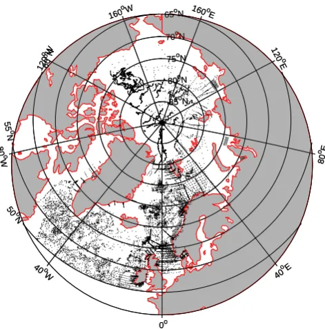
The map of locations of assimilated in-situ observations North of 50◦N for the period from April 2007 to Decem-ber 2009 is shown in Fig. 4.
The ICEC data is obtained from AMSR-E. It is com-puted with the ARTIST sea-ice concentration algorithm us-ing AMSR-E 89 GHz brightness temperatures. The grid-ded data is available from 19 June 2002 at a resolution of 12.5 km. The spatial coverage is almost complete. TOPAZ4 assimilates the ICEC data on the day of each analysis. The observation error standard deviation is set to 10 % at the start of the reanalysis and is increased on 25 January 2006 to ac-count for larger errors near the ice edge and to reduce over-fitting at these locations. The error variance then becomes:
σobs2 =0.01+(0.5− |0.5−c|)2,
160 oW 120 oW 80 o W 40 o W 0o 40 oE 80 oE 120 o E 160o E 50 o N 55 o N 60 oN
65oN
70oN
75oN
80oN
85oN
160 oW 120 oW 80 o W 40 o W 0o 40 oE 80 oE 120 o E 160o E 50 o N 55 o N 60 oN
65oN
70oN
75oN
80oN
85oN
Fig. 4. The map of locations of assimilated in-situ observations north of 50N for the period from April 2007 to December 2009.
The sea-ice drift product is provided by CERSAT, Ifremer (Ezraty et al., 2006). The Lagrangian drift data is obtained at a resolution of 35 km by a pattern recognition algorithm from QuickSCAT, AMSR-E and SSM/I images. It is avail-able from October to April inclusive and does not provide in-formation close to the ice edge. The 3-day drift has been cho-sen as a compromise: long enough to average out some ran-dom errors in the composites that are computed over shorter periods and short enough to avoid severe loss of data near the coast that occurs in the composites computed over longer periods. The data is available from October 2002, but it is un-available during summer due to loss of patterns where melt-ing occurs. The provider accuracy estimate of 7 km/3 days is overestimated by a factor 2 to account for representation error.
Because the sea-ice drift data is Lagrangian, the cor-responding observation operator is nonlinear. The model equivalent 3-days drift is computed for each ensemble mem-ber and each grid cell of the satellite data product. The initial positions are advected 3 days forward using model daily av-eraged ice velocities and a 2nd order Runge-Kutta method. The final displacements are computed on the observation grid.
4.3 Bias estimation
Bias estimation of SST and mean sea surface height (MSSH) was implemented in the reanalysis in February 2008. The fol-lowing is a brief description of the bias estimation procedure.
1. The bias fields for each ensemble member are ini-tialised to random spatially uniform values, with the standard deviation of the order of expected bias mag-nitude (the SST bias fields were initialised in the inter-val[−4,4]◦C; the MSSH bias fields –[−0.6,0.6]m). There is no need to have spatial variations in the initial fields due to the use of localisation.
2. These fields are then augmented to the state vector. 3. During assimilation, the forecast observations for each
ensemble member are offset by the value of the cor-responding bias field. This involves SLA and SST ob-servations, as well as in-situ temperature obob-servations, which are offset up to the model depth of the mixed layer for a given ensemble member, with a smooth tran-sition between offsetting by the full magnitude of the SST bias and no correction at about the mixed layer depth.
4. The bias fields are corrected due to their correlations with the forecast ensemble observations, which estab-lish after a few assimilation cycles.
5. The bias fields remain constant during propagation, but their spread reduces after each assimilation cycle. Therefore, to avoid collapse of bias field ensembles, ad-ditional inflation is introduced (2 % per cycle for SLA, and 6 % for SST).
This bias estimation procedure is similar to that in the EnKF-Matlab package available from http://enkf.nersc.no/Code/ EnKF-Matlab.
The difference in the magnitude of inflation for the SST and MSSH bias field is due to the fact that, as indicated by the innovation statistics, the SST bias has seasonal variabil-ity; while SLA is supposed to have substantial constant or interseasonal component.
Note that the bias correction doesn’t explicitly correct the model bias, but rather diagnoses it. As a consequence, the best model estimate is the reanalysed state plus the diag-nosed time-dependent bias. Also note that in TOPAZ4, the bias estimates are subtracted from the innovation, so that a well-behaved bias estimate reduces, on average, the innova-tion magnitude.
5 Results
5.1 Innovation statistics
Table 2. Boxes used for innovation statistics (see also Fig. 1).
Box ID Box name Min. lon. Max. lon. Min. lat. Max. lat.
1 Nordic Seas −30 20 63 80
2 Gulf Stream Extension −50 −15 40 60
3 Gulf Stream −80 −40 30 45
4 Tropical −60 −15 0 20
5 Arctic −180 180 70 90
2004 2006 2008
−0.1 −0.05 0 0.05 0.1
Nordic Seas box
0 1000 2000 3000 4000
2004 2006 2008
0 0.05 0.1 0.15
Gulf Stream Extension box
0 2000 4000 6000
2004 2006 2008
0 0.05 0.1 0.15 0.2 0.25
Gulf Stream box
0 1000 2000 3000 4000
2004 2006 2008
0 0.05 0.1
Tropical box
0 2000 4000 6000
bias RMSD σens σtot # obs.
Fig. 5. Time series of regionally-averaged innovation statistics for satellite-derived SLA observations, including the bias (mean observed minus mean background; negative innovation bias corresponds to a warmer model), the RMSD between the observations and the model background field of the innovation, the ensemble spreadσens, and the estimated standard deviation of the innovationσtot(the quadrature sum
ofσensand the assumed standard deviation of the observation errors). The boundaries to the regions are denoted in Fig. 1. The number of
observations assimilated is also shown (grey line) with its corresponding axis on the right-hand-side of each panel. The Arctic region is not represented because there are no reliable remote SSH observations there.
In each case, time series are shown for the model bias (la-belled bias); the root-mean-squared difference (RMSD) be-tween the observations and the model background field (la-belled RMSD); the standard deviation of ensemble anoma-lies (labelled σens) that represents an estimate of the back-ground error standard deviation; the estimated standard de-viation of the innovation (labelledσtot) that is the quadrature sum ofσensand the assumed observation error standard
devi-ationσobs; and the number of observations to be assimilated (labelled # obs.).
2004 2006 2008 −2
−1 0 1 2
Nordic Seas box
0 2000 4000 6000 8000 10000
2004 2006 2008
−1 −0.5 0 0.5 1 1.5
Gulf Stream Extension box
0 0.5 1 1.5 2
x 104
2004 2006 2008
−1 0 1 2
Gulf Stream box
0 0.5 1 1.5 2
x 104
2004 2006 2008
−1 −0.5 0 0.5 1
Tropical box
0 1 2 3 4
x 104
bias RMSD σens σtot # obs.
Fig. 6. Innovation statistics for SST (see description in caption to Fig. 5). The Arctic region is not represented because there are no remote SSH observations there.
and meanders, where the “shape” and phase of features in the ocean are important.
The time series of the innovation statistics for SLA (Fig. 5) show that the RMS of the innovations remained fairly con-stant throughout the reanalysis. These time series indicate that the RMS error for SLA is about 0.05 m in the Nordic Seas box; between 0.07 and 0.09 m in the Gulf Stream Exten-sion box; between 0.13 and 0.18 m in the Gulf Stream box; and about 0.04 m in the Tropical box. We note a substantial seasonal bias in the Nordic Seas box, and to a lesser degree, in the Gulf Stream Extension box. The SLA innovation bias in the Nordic Seas box seems to exceed, on average, the es-timated amplitude of seasonal steric height anomaly in the Nordic Seas (Siegismund et al., 2007, Fig. 5).
Generally, there is a good agreement between the esti-mated innovation standard deviationσtot and the measured RMSD for all presented fields. This demonstrates an internal consistency between the background and observation error variance and the innovations.
With regard to the innovation statistics for SST (Fig. 6), the RMSD of the innovations fluctuate throughout the pe-riod of the reanalysis, with a peak each year that corresponds
to a peak in the magnitude of the bias. This seasonal be-haviour of the bias and RMSD is clearly seen in all boxes, except, perhaps, the Tropical box where the seasonality is weaker. The magnitude of the bias and the RMS are often comparable. This indicates that the RMSD between the re-analysed and observed SST is often dominated by the bias. In February 2006, the assimilated SST data was switched from Reynolds SST to OSTIA. The timing of this switch is evident in Fig. 6, when the number of observations increases signif-icantly. The RMSD and bias decrease after this transition, indicating that the OSTIA SST is better suited to constrain-ing the TOPAZ system. Prior to 2006, the RMS of the SST innovations in the Nordic Seas, Gulf Stream Extension, Gulf Stream and the the Tropical boxes is typically between 1.1– 1.8◦C, 0.7–1.2◦C, 1–1.5◦C, and 0.6–1.0◦C, respectively. After OSTIA SST data started to be assimilated the RMSD of the SST innovations dropped to 0.5–0.8◦C, 0.5–1.0◦C (with
the exception of the peak in summer 2006), 0.7–1.3◦C, and
0.4–0.5◦C in the Nordic Seas, Gulf Stream Extension, Gulf Stream, and Tropical boxes, respectively.
2003 2004 2005 2006 2007 2008 2009 −0.15
−0.1 −0.05 0 0.05 0.1 0.15 0.2 0.25 0.3 0.35
Arctic box
0 0.5 1 1.5 2 2.5 3 3.5 4 4.5 5 x 10⁴
bias RMSD σens σtot # obs.
Fig. 7. Innovation statistics for ICEC (see description in caption to Fig. 5).
dashed vertical line. It is also marked by a sharp increase in the ensemble spread that includes the uncertainty in the bias. Although the bias estimation period is relatively short, the SST bias seems to decreases significantly after this point in the Gulf Stream and Tropical boxes, and decreases to some degree in the Nordic Seas and Gulf Stream Extension boxes; the RMS of the innovations also reduces after the bias is ex-plicitly diagnosed and accounted for. Interestingly, the SST bias field does not show as much seasonal variability (not shown) as the bias of the SST innovations. This suggests that the seasonality of the SST bias that is evident in Fig. 6 may be related to the seasonal variations in the surface mixed layer depth. The surface mixed layer is generally deeper in winter. This is reflected in the ensemble-based background error co-variance (not shown) that projects the SST innovations over a greater depth in winter. As a result, during winter, it appears that the assimilation of SST data better constrains the ocean model.
The vertical dashed red line in Fig. 6 denotes the time when the variance increasing factor of 2 for the update of the ensemble anomalies, described in Sect. 3.2, was intro-duced. It is expected to result in the increase of the ensemble spread and therefore the sensitivity of the DA system to ob-servations. The impact on the ensemble spread is evident in Figs. 5 and 6, but any change in the sensitivity of the analysis system to individual observations is less clear. We suspect a
parallel run without the variance increasing factor is needed to quantify this sensitivity.
The ensemble spread for SST remains relatively constant throughout the reanalysis for all domains considered here, indicating that the DEnKF showed no tendency towards en-semble collapse. It shows some seasonal fluctuations in each box except the Tropical box, with greater spread in winter and less in summer.
For an optimal data assimilation system,σtotshould match the RMS of the innovations. Clearly, for SST prior to the switch to OSTIA SST,σtot was too small by about 50 % of the RMS, but was approximately correct after the switch to OSTIA. This indicates that either the ensemble spread,σens, was too small before the switch to OSTIA, or the assumed observation errors for Reynolds SST were too small. We sus-pect that the latter is true. The consistency between the actual innovation, given by the RMSD, and the estimated innova-tion, given byσtot, demonstrates a consistency between the assumed and computed background and observation errors, and the actual errors of the background fields in the reanaly-sis.
Fig. 8. Estimated MSSH and SST bias fields at the end of the reanalysis (after 10 months of estimation). Regions with no observations available at that time are masked to 0. Positive bias corresponds to a higher model MSSH/SST compared to observations.
summer can be seen in Fig. 7 when the number of observa-tions assimilated substantially decreases and then increases again, reflecting the ice extent. Note the strong correlation between the RMSD and the bias. This indicates that a signif-icant portion of the RMSD is attributed to the bias.
The vertical dashed black line marks the time when a num-ber of changes have been introduced into the system after ob-serving some excessive increments in salinity in the course of assimilating ICEC. These changes include the introduction of adaptive observation pre-screening (Sect. 4.2), increasing the perturbations of model forcing to affecting the position of the ice edge (Sect. 3.3), and relaxation of the assumed obser-vation error variance (Sect. 4.2). These changes seem to im-prove the performance of the system in regard to the ICEC. For example, there is an increasing trend in the RMSD prior to the change, which is then reversed.
The time series of ensemble spread shows a peak each summer that is in phase with the peak in RMSD. Moreover, the time series of the estimated standard deviation of the in-novationσtotis remarkably well-aligned with the RMSD.
This demonstrates an internal consistency between the ac-tual errors, quantified by the RMSD, and the assumed and modelled estimates of the errors, from the estimated obser-vation errors and the ensemble-based estimate of the back-ground field errors. This is a very encouraging result, be-cause it demonstrates that the time-varying estimate of the background field errors from the ensemble can be used to quantify the error in the system in advance. This internal
con-sistency and functionality is highly desirable for every data assimilation system – but it is rarely achieved in practice.
5.2 Bias estimates
The estimated bias fields for MSSH and SST at the end of reanalysis are presented in Fig. 8. An assessment of the bias estimate for MSSH is provided in Fig. 10, where we com-pare the MSSH derived from TOPAZ before the bias cor-rection is introduced (from a free run of the model), after the bias is introduced (from the reanalysis), and the observations-only MDT from CNES-CLS09 (Rio et al., 2009), not assim-ilated. The revised MSSH after the bias is introduced is con-structed by adding the time-mean estimate of the SSH bias with the MSSH from the free model run. Several aspects of the revised MSSH are in better agreement with CNES-CLS09 MDT than the MSSH from the free model run. For example, the Gulf Stream at Cape Hatteras shoots too far north in the free model run, as one expects from a model of this resolution, is shifted southwards and is more confined in the revised MSSH. The improvement is visible in the merid-ional section at 60◦W in Fig. 9, where the MSSH drop south
Fig. 9. Sections of MDT from Rio09 (black), HYCOM free run (blue), and estimated with data assimilation (green). An offset of 15 cm has been removed from the Rio09 data.
a) b)
c)
Fig. 10. (a) TOPAZ4 MSSH before bias correction; (b) TOPAZ4 MSSH after bias correction; (c) MDT from CNES-CLS09.
Gyre that is evident in CNES-CLS09 MDT is also evident in the revised MSSH, but is not clear in the original MSSH.
Fig. 11. Drifter trajectories in the Gulf Stream box (dots) versus the analysis SSH. The drifter positions are plotted at 6 h time step within±4 days from the day of the analysis (given at the top of each panel).
strong in the original MSSH. This is also illustrated in the meridional section at 20◦W in Fig. 9: the downward slope
between 40◦N and 60◦N is steeper after bias estimation, in
better agreement with the observations. Here again, the cor-relation increases from 0.86 to 0.92.
An attractive aspect of the online bias estimation is that it requires no hand-tuning of the MSSH. The joint assimi-lation of satellite observations and in-situ Argo temperature and salinity profiles (mostly in-situ data) are solely responsi-ble for the corrections to the MSSH.
The SST bias field (Fig. 8) shows several regions of spa-tially coherent positive bias, including regions in the Gulf of Mexico and the Caribbean Sea, the southern part of the sub-Tropical Gyre and parts of the Mediterranean Sea. In these areas the model is warmer, indicating either that the net sur-face heat flux is too high or that the modelled sursur-face mixed layer is too shallow – so that not enough sub-surface water is entrained into the surface layers. There are also several regions along the path of the Gulf Stream Extension where
the SST bias is large and negative. We suspect that this is an indication that the path of the Gulf Stream is too far to the south.
5.3 Comparison with drifting buoys
0 0.1 0.2 0.3 0.4 0.5 0.6 0.7 0.8 0.9 1
Fig. 12. Monthly average ICEC reanalysis fields for for April (two top rows) and September (two bottom rows). The thick black line shows the 15 % concentration contour derived from the monthly average observation based ICEC from AMSR.
between the SSH fields in the reanalysis and the independent observations of drifter paths. In many cases, even the details of the drifter paths are well captured by the reanalysis.
The good comparisons between drifter paths and modelled SSH demonstrates that the TOPAZ system produces
Fig. 13. Average fields for the ice thickness for October–November; for observations from ICESat (Kwok and Rothrock, 2009), free run and reanalysis. The red line shows the contour of 15 % ICEC from AMSR data.
the focus of the TOPAZ developments is the Arctic Ocean, not the North Atlantic Ocean.
We note that a similar comparison between drifter paths and the free running model without data assimilation shows no correspondence between individual mesoscale features in the model and observations (not shown). This is what we ex-pect, and is a consequence of the chaotic nature of mesoscale
a)
b)
c)
Fig. 14. Mean monthly SSS: (a) for January 2007 by TOPAZ4; (b) January 2008 by TOPAZ4; (c) for January from PHC climatology.
a)
b)
c)
Fig. 15. Mean monthly salinity at 100 m: (a) for January 2007 by TOPAZ4; for January 2008 by TOPAZ4; (c) for January from PHC climatology.
5.4 Evaluation of ice fields
To demonstrate the quality of ICEC field in the reanalysis, we show in Fig. 12 comparisons between the monthly aver-age reanalysed ICEC and monthly averaver-age ice edge contour drawn at 15 % of ICEC based on the AMSR data. The data are presented for April and September, which represent the months with maximal and minimal total sea ice extent.
The correspondence of the reanalysed and observed sea ice extents is generally quite good, except September of 2005 and 2006, when the model produced too much sea ice. These periods can also be in the RMSD of the innovation of ICEC in Fig. 7; however, we note that the RMSD seem to peak somewhat earlier in the year. We note that the sea ice extent in TOPAZ is particularly good off eastern Greenland and off Spitsbergen (Svalbard). These regions are key regions of in-terest for many applications. The Fram Strait is the only deep passage between the Arctic and the and the rest of the Worlds Oceans. The crossing of the North Atlantic and Arctic waters
needs to be monitored as well as the export of sea ice from the central Arctic into the Greenland Seas, which depletes the ice pack (Kwok, 2009).
The comparisons of early Fall ice thickness in Fig. 13 show that the data assimilation has done limited change to the overall distribution of ice in the Arctic, in line with Lisæter et al. (2003) who found that the assimilation of ice concentra-tions mostly impacted the position of the ice edge, but not so much the ice volume. The ice is too thin in areas of thick ice and inversely, too thin in areas of thick ice, which is a com-mon feature in models that use a viscous rheology (Johnson et al., 2012). The assimilation has indeed slightly thickened the ice there, which – by elimination – is likely to be the ef-fect of assimilating ice drift. The ice is also thickened to the North of Franz Joseph Land and Siberian Islands, in better agreement with the ICESAT data, which reflects the better position of the ice edge during the ice minimum.
reveals that the model ice drift is generally slightly too fast, by 3 km day−1for slow drift as much as for fast drift, which is a known deficiency of the EVP type of model: Girard et al. (2009) reported an even larger bias of 6 to 7 km day−1. The too fast ice drift is advecting too much ice into the Beaufort Sea and is consistent with the ice pack being spread out, as mentioned above.
5.5 Evaluation of salinity and temperature
Below we will mainly concentrate on the evaluation of salin-ity, which is the most important tracer for circulation in the Arctic; but we will also provide some temperature compar-isons with mooring data.
A comparison of SSS from the TOPAZ reanalysis, from the GDEM climatology (Teague et al., 1990), and from a free run of the model (not shown) indicates that these SSS fields are very similar in the North Atlantic. By contrast, there is a significant improvement in the SSS of the reanalysis in the Arctic compared to that of the free running model.
Figures 14 and 15 show the monthly mean SSS and the monthly mean salinity at 100 m depth (S100) for the reanal-ysis during January 2007, before in-situ observations in the Arctic are assimilated, and during January 2008, after in-situ observations in the Arctic are assimilated. For comparison, we also show an estimate of SSS climatology from PHC (Steele et al., 2001).
The SSS and S100 fields in January 2007, before in-situ observations in the Arctic are assimilated, show an unreal-istically large and misplaced Beaufort Gyre, with too low salinity. The salinity of the free run is very similar to that of the reanalysis in January 2007 (not shown). In spite of this model deficiency, the intensity and location of the Beaufort Gyre are corrected efficiently by assimilation of the profiles. We interpret this improved performance in 2008 as an indica-tion that the assimilaindica-tion of in-situ observaindica-tions in the Arctic is beneficial, and has had a measurable positive impact on the reanalysis (however, see Sect. 5.8 in regard to the patchiness observed in the middle panels of Figs. 14 and 15).
In particular, the assimilation of ITP profiles appears to be critical for constraining the central Arctic temperature and salinity structures, even though the number of ITP profiles was limited. Indeed, the total DFS and SRF, presented in Fig. 3, show that the efficiency of these profiles under ice is very high compared to other observations in the high lat-itudes, confirming that these data had a very significant im-pact on the reanalysis.
The temperature and salinity profiles in the Arctic are as-sessed against the NABOS/CABOS moorings in Fig. 16. The moorings were active before the assimilation of ITP data but not assimilated. The temperature profiles in the Laptev Sea reveal insufficient transport or excessive diffusion of warm Atlantic Water. Although transport estimate in the Fram Strait compares well with observations(see Sect. 5.7), the core of Atlantic Water is too weak and too diffuse (see
Sect. 5.6). This excessive diffusion may result from the arti-ficial thickness diffusion used for model stability or from our parametrisation of diapycnal mixing that does not account for the attenuation of internal waves below sea ice (Morison et al., 1985; Nguyen et al., 2009).
For the Canadian mooring the comparison with observa-tions for both the reanalysis and the free run is quite poor. Note, however, that historically TOPAZ has been calibrated for the North Atlantic and the adjacent Arctic sector rather than for the Canadian basin. Both simulations show a too shallow and too cold Pacific Water, which is likely to be a direct consequence from disregarding seasonal variability in the Bering Strait inflow. The reanalysis does not show the Atlantic layer presented in observations, and in this instance, the free running model is closer to observations. However, in view of the relatively patchy horizontal fields (not shown), we suspect the deterioration of the reanalysis to be an iso-lated case rather than reflecting a general tendency.
5.6 Comparison with hydrographic sections
The Fram Strait is the main oceanic gateways between the Atlantic and the Arctic Ocean and is thus the most impor-tant region for the exchange of Atlantic and Polar water masses. Since 1997 oceanic fluxes through Fram Strait have been monitored by an array of moorings deployed between 6◦300W and 8◦400E at the latitude 78◦500N (Schauer et al., 2008; Beszczynska-M¨oller et al., 2011). This data-set is not assimilated during the pilot reanalysis and can be thus con-sidered as independent. Several water masses are present in the Fram Strait. Near the surface on the eastern side, there are several branches of the warm and saline Atlantic Wa-ter (inflow and recirculation). On the wesWa-tern side the East Greenland Polar front englobe the fresh and cold Polar Wa-ter. Between 800 m and 1200 m, one can find the Arctic Inter-mediate Water and the Upper Polar Deep Water with a tem-perature close to 0◦C. Bellow, the Nordic Sea Deep Water and the Arctic Ocean Deep Water are present.
Figure 17 compares temperature from the free and assim-ilative runs to the data in the winter and summer 2007. The improvements from data assimilation are numerous. The At-lantic Water in the free run is too cold, too deep and diffuse. This is much improved in the reanalysis even if the multiple cores are not clearly represented and the core of Atlantic Wa-ter is still too deep and slightly too diffuse. The Polar WaWa-ter is also too deep in the free run. In the reanalysis the water is located at a reasonable depth but extends too far to the east. Both the free run and the reanalysis misrepresent the deep water. The differences in the intermediate and deep water are small, but the stratification is better pronounced in the reanal-ysis and the deep water is slightly colder. It appears that the influence of data assimilation at depths is minor.
30 31 32 33 34 35 0
500
1000
1500
salinity
depth [m]
Laptev Sea mooring, 2005−2006
(a)
observations TOPAZ
free run 2003−2008 PHC climatology
−2 −1 0 1 2
0
500
1000
1500
temperature [ oC]
depth [m]
Laptev Sea mooring, 2005−2006
(b)
28 30 32 34 36
0
200
400
600
800
1000
1200
salinity
depth [m]
Canadian mooring, 2006−2007
(c)
−2 −1 0 1
0
200
400
600
800
1000
1200
temperature [ oC]
depth [m]
Canadian mooring, 2006−2007
(d)
Fig. 16. Salinity (a, c) and temperature (b, d) profiles for the Canadian mooring C1F (71.50◦N, 131.47◦W) and Laptev Sea mooring M1C (78.43◦N, 125.61◦E), compared with PHC climatology, free model run and reanalysis; all data is averaged over the observation period (C1F: 12 September 2006–28 August 2007; M1C: 15 September 2004–15 September 2005).
spin-up), the water masses are in better agreements to obser-vations than in the free run started the initialisation problem.
5.7 Volume transport estimates
Time series of 3-monthly averaged volume transports through the Svinøy section and Barents Sea Opening (de-noted in Fig. 1), from the reanalysis and from independent observations, is presented in Fig. 18. The Svinøy section is a key location for measuring the Atlantic inflow to the Norwe-gian Sea, due to the topographic steering of the NorweNorwe-gian Atlantic Slope Current (NwASC) and its vertical structure. Skagseth et al. (2008) estimate the volume flux from one sin-gle mooring in the core of the flow. After passing through the Svinøy section, the NwASC flows northwards into the Arctic and splits in two branches between Norway and the Spitsber-gen and between the Barents Sea Opening (BSO) and the West Spitsbergen Current (WSC). Another array of moored current measurements in the BSO monitors the fluxes be-tween Norway and Bear Island (Ingvaldsen et al., 2004). The associated uncertainty estimates are not provided in either case, but differences should be expected between the
punc-tual current measurements and the section-averaged volume fluxes, even after low pass filtering. The velocity measure-ments used to generate the observational estimates of the volume transport in Fig. 18 were not assimilated in the re-analysis.
In the Svinøy section, the transport estimate from the free run is too low (3.5 Sv) compare to observation (4.7 Sv) and the one from the reanalysis is too high (6.1 Sv). The free run transport is too low until 2005, but then adjusts to a level that is comparable to the observation while the reanalysis trans-port remains offset during the whole integration. The vari-ability is relatively well captured by the model but the reanal-ysis correlates better with the observations, with the correla-tion coefficient increasing from 0.7 to 0.8. Both model runs represent reasonably well the seasonal variably but the in-terannual variability of the volume transports is better repro-duced by the reanalysis with an increasing trend until 2006, followed by a decreasing trend.
Fig. 17. Temperature in the Fram Strait section from the free run, reanalysis and observations.
2004 2005 2006 2007 2008
−1 0 1 2 3 4 5 6 7 8 9
Svinoy
Obs Free run Reana
2004 2005 2006 2007 2008
0 1 2 3 4 5 6 7
BSO
Obs Free run Reana
Fig. 18. Comparison of 4-monthly average transport through the Svinøy section and Barents Sea Opening section from observations, free model run and TOPAZ reanalysis.
this difference to insufficient resolution in the surface forcing fields (from ERA-interim) that does not accurately represent winter storms and polar lows. The transport is overestimated in both the free run and the reanalysis (with 2.9 Sv instead of 2.2 Sv from observations). Still, the free and assimilated run are very close to each other and reasonably close to the observations with respect to other model products of higher resolution (Gammelsrød et al., 2009).
Finally, the transport in the Fram Strait is analysed against the estimate from Mauritzen et al. (2011) computed between 2002 and 2008. The net Southward transport is respectively
2.3 Sv and 2.2 Sv for the free run and reanalysis, well in line with the observed transport of 2.08 Sv.
Overall, the magnitude of the volume transport in the re-analysis in the Svinøy section, BSO and Fram Strait are in good agreement with the observed estimates. This indicates that the partitioning of the current between the NwASC, the BSO, and WSC is well reproduced in the reanalysis.
the course of the pilot reanalysis did not abruptly impact the reanalysed circulation in the Nordic Seas.
The coverage of the observation network also changes over time, including the addition of Argo profiles in the Nordic Seas in early 2007. We did not find that this change results in any significant change of the circulation, although the assimilation of Argo profiles may have improved the fit of the volume transport in the Svinøy section in 2008 com-pared to the previous years (Fig. 18), but a longer integration is needed to be sure of this result.
5.8 Known problems
After completing the reanalysis, a problem was identified in the superobing code for in-situ temperature and salinity ob-servations that affected a small proportion of in-situ observa-tions for the Arctic and Nordic Seas during 2007 and 2008. We believe that this issue had no major impact on the re-analysed fields due to the small amount of erroneous obser-vations (less than 1 %) and due to the adaptive observation pre-screening procedure (Sect. 3.2); however, we found that this error causes some instances of patchiness in the reanal-ysed fields in the Arctic.
A hardware (Input/Output) problem has been identified that has affected the system in November 2002, before the start of the reanalysis. The most obvious impact was an anomalously wide Beaufort Gyre containing too much fresh water. In order to assess only the impact of assimilation, the free run has been initiated after the November 2002 problem. In the course of the reanalysis, and with the assimilation of the ITP profiles, the Beaufort Gyre was restored to a rea-sonable size, though several imperfections remain visible, far from the ITPs locations.
Some model parametrisations were also found inappropri-ate. A constant inflow in the Bering Strait leads to biased fresh water and heat fluxes (Ness et al., 2010). The inflow of Atlantic Water in the Fram Strait is diffuse supposedly because the diapycnal mixing and layer thickness diffusion were not calibrated specifically for the Arctic.
6 Conclusions
The purpose of this paper is to provide a description and eval-uation of TOPAZ4, the latest version of TOPAZ – a coupled ocean-sea ice data assimilation system for the North Atlantic Ocean and the Arctic. TOPAZ is the only operational, large-scale ocean data assimilation system that uses the EnKF. The version of the EnKF used in TOPAZ4 is the DEnKF (Sakov and Oke, 2008a). We show that the state-dependence of the background error covariance is particularly important for a coupled ocean-sea ice system because of the strong non-stationarity and anisotropy of correlations between physical fields across the ice edge. This sets the current application apart from many other short-range ocean forecast systems
that are developed for open ocean forecasting, and not cou-pled ocean-sea ice forecasting.
We provide an evaluation of TOPAZ4 through a pilot MyOcean reanalysis that spans the period 2003–2008. We demonstrate that TOPAZ4 produces a realistic estimate of the ocean circulation in the North Atlantic and the sea ice variability in the Arctic. One of the potential strengths of any EnKF-based data assimilation system is that it predicts and evolves the system’s state error covariance implicitly in the ensemble, as well as the system’s state. Thus, it provides an estimate of the system errors in real time. We evaluate this aspect of the TOPAZ4 system by analysing the innovation statistics of the reanalysis. We find that the ensemble-based estimate of the background error variance for SST and SSH remain fairly constant throughout the reanalysis and that, af-ter accounting for the system’s bias, this is consistent with the misfits between the model fields and the assimilated ob-servations. We also find that the variance of the ensemble – the system’s online “prediction” of the background error variance – for ICEC is well correlated with the misfits be-tween the model and observations. This result demonstrates that the ensemble statistics could be reliably used to obtain state-dependent error estimates for the system – a feature that is unique to ensemble-based data assimilation systems.
During the course of the reanalysis, we introduce various modifications to the assimilation configuration, and to the ob-servations assimilated. For example, we switch the source of SST data that is assimilated, and we introduce an explicit on-line bias estimation. We recognise that this approach is not systematic, and leaves some uncertainty about the specific impact of each of these changes. However, the cost of per-forming an independent reanalysis to evaluate the impact of each and every modification is prohibitively expensive, and is probably not warranted. Despite this, we can infer the impact of the modifications by analysing the changes in the perfor-mance of the reanalysis before and after each modification. In some cases, the impact of the introduced changes are clear. For example, the quality of the reanalysis changes when dif-ferent SST products are assimilated. When we switch from a Reynolds SST product to OSTIA, we see an immediate and measurable improvement in the system’s performance. We also find that when in-situ T and S profiles from below the ice in the Arctic Ocean are assimilated, the system’s perfor-mance also improves, and we therefore plead for a continua-tion of the ITPs after the end of the IPY.
The evaluation of volume transport through key sections also reveals a correct circulation in the Nordic Seas, which is a necessary prerequisite for modelling the Arctic.
The latest version of TOPAZ includes many changes com-pared to its predecessor, including a new data assimilation scheme, improvements to many aspects of the configuration of the data assimilation, the assimilation of different observa-tion types, and improvements to the underlying ocean model. Through the pilot reanalysis that we present here, we demon-strate the benefits of these changes and the improvements to the TOPAZ system.
At the same time, verification of the pilot reanalysis clearly identifies the areas for improvement of the system. The water masses in the Arctic in the reanalysis are substantially dif-ferent from observations from NABOS/CABOS moorings. Specifically, Fig. 16 shows weak or absent Atlantic layer, which points at insufficient Northwards advection through the WSC. While the state of the water masses can be im-proved by assimilating observations from in-situ profiles, assimilation does not replace a careful model calibration, which can have a major impact on the quality of water masses modelling in the Arctic (Nguyen et al., 2011) even in the ab-scence of data assimilation.
The multivariate impact of data assimilation has been anal-ysed by comparing the reanalysis and free model with in-dependent data sets. The comparisons show improvements for ice thickness and salinity in the Arctic; and substan-tial improvement for temperature in the Fram Strait. There are slight improvements for transport estimates across the Svinøy section, but not for the the Barents Sea Opening. Compared with mooring data, there are slight improvements for underwater temperature in the Laptev Sea, but a degra-dation in the Beaufort Sea. Overall we can believe that this confirms the skill of the EnKF in the Arctic that has been already demonstrated in Lisæter et al. (2003).
Through a 6-year pilot reanalysis, we demonstrate that TOPAZ4 produces a realistic representation of the mesoscale ocean circulation in the North Atlantic, and a realistic rep-resentation of sea ice variability in the Arctic. In Septem-ber 2010, an almost similar TOPAZ4 system was imple-mented operationally at met.no and produces 10-day fore-casts every day. Results from the operational version of TOPAZ4 are available at http://myocean.met.no, and output from the pilot reanalysis are available at http://topaz.nersc. no.
Acknowledgements. The authors gratefully acknowledge support from the eVITA-EnKF project by the Research Council of Norway; from the MyOcean project by EU; and by a grant of CPU time from the Norwegian Supercomputing Project (NOTUR2). The observations from IMR, IOPAS, ICES, MMBI, AARI, were assembled and quality checked within the project.
Edited by: P. Brasseur
References
Antonov, J., Locarnini, R., Boyer, T., Mishonov, A., and Garcia, H.: World Ocean Atlas 2005 Volume 2: Salinity, NOAA Atlas NESDIS, 62, 182 pp, 2006.
Bentsen, M., Evensen, G., Drange, H., and Jenkins, A. D.: Coordi-nate transformation on a sphere using conformal mapping, Mon. Weather Rev., 127, 2733–2740, 1999.
Bertino, L. and Lisæter, K. A.: The TOPAZ monitoring and predic-tion system for the Atlantic and Arctic Oceans, Journal of Oper-ational Oceanography, 2008, 15–18, 2008.
Beszczynska-M¨oller, A., Woodgate, R. A., Lee, C., Melling, H., and Karcher, M.: A synthesis of exchanges through the main oceanic gateways to the Arctic Ocean, Oceanography, 24, 82–99, 2011. Bishop, C. H., Etherton, B., and Majumdar, S. J.: Adaptive sampling
with the ensemble transform Kalman filter. Part I: theoretical as-pects, Mon. Wea. Rev., 129, 420–436, 2001.
Bleck, R.: An oceanic general circulation model framed in hybrid isopycnic-Cartesian coordinates, Ocean Model., 4, 55–88, 2002. Bonavita, M., Torrisi, L., and Marcucci, F.: The ensemble Kalman filter in an operational regional NWP system: preliminary results with real observations, Q. J. R. Meteorol. Soc., 134, 1733–1744, 2008.
Brasseur, P., Bahurel, P., Bertino, L., Birol, F., Brankart, J.-M., Ferry, N., Losa, S., Remy, E., Schr¨oter, J., Skachko, S., Testut, C.-E., Tranchant, B., Van Leeuwen, P. J., and Verron, J.: Data assimilation for marine monitoring and prediction: The MER-CATOR operational assimilation systems and the MERSEA de-velopments, Q. J. R. Meteorol. Soc., 131, 3561–3582, 2005. Brusdal, K., Brankart, J., Halberstadt, G., Evensen, G., Brasseur, P.,
van Leeuwen, P. J., Dombrowsky, E., and Verron, J.: An eval-uation of ensemble based assimilation methods with a layered OGCM, 40-41, 253–289, 2003.
Burgers, G., van Leeuwen, P. J., and Evensen, G.: Analysis scheme in the ensemble Kalman filter, Mon. Wea. Rev., 126, 1719–1724, 1998.
Canuto, V., Howard, A., Cheng, Y., and Dubovikov, M.: Ocean tur-bulence. Part II: Vertical diffusivities of momentum, heat, salt, mass, and passive scalars, Journal of Physical Oceanography, 32, 240–264, 2002.
Cardinali, C., Pezzulli, S., and Andersson, E.: Influence-matrix di-agnostic of a data assimilation system, Q. J. R. Meteorol. Soc., 130, 2767–2786, 2004.
Cavalieri, D., Parkinson, C., Gloersen, P., and Zwally, H.: Sea ice concentrations from Nimbus-7 SMMR and DMSP SSM/I pas-sive microwave data, CD-ROM. National Snow and Ice Data Center, Boulder, CO, USA, 1999.
Chassignet, E., Hurlburt, H., Smedstad, O., Halliwell, G., Hogan, P., Wallcraft, A., and Bleck, R.: Ocean prediction with the hybrid coordinate ocean model (HYCOM), Ocean Weather Forecasting, pp. 413–426, 2006.
Chassignet, E. P., Hurlburt, H. E., Smedstad, O. M., Halliwell, G. R., Hogan, P. J., Wallcraft, A. J., Baraille, R., and Bleck, R.: The HYCOM (HYbrid Coordinate Ocean Model) data assimila-tive system, J. Marine Syst., 65, 60–83, 2007.