SRef-ID: 1607-7946/npg/2005-12-741 European Geosciences Union
© 2005 Author(s). This work is licensed under a Creative Commons License.
Nonlinear Processes
in Geophysics
Role of the hydrological cycle in regulating the planetary climate
system of a simple nonlinear dynamical model
K. M. Nordstrom1, V. K. Gupta2,3, and T. N. Chase2,4
1Colorado Research Associates, 3380 Mitchell Lane, Boulder, Colorado 80301, USA
2Cooperative Institute for Research in the Environmental Sciences, University of Colorado, Boulder, Colorado 80309, USA 3Department of Civil and Environmental Engineering, University of Colorado, Boulder, Colorado 80309, USA
4Department of Geography, University of Colorado, Boulder, Colorado 80309, USA
Received: 12 July 2004 – Revised: 15 March 2005 – Accepted: 16 March 2005 – Published: 29 July 2005
Part of Special Issue “Nonlinear deterministic dynamics in hydrologic systems: present activities and future challenges”
Abstract. We present the construction of a dynamic area
fraction model (DAFM), representing a new class of mod-els for an earth-like planet. The model presented here has no spatial dimensions, but contains coupled parameteriza-tions for all the major components of the hydrological cy-cle involving liquid, solid and vapor phases. We investigate the nature of feedback processes with this model in regu-lating Earth’s climate as a highly nonlinear coupled system. The model includes solar radiation, evapotranspiration from dynamically competing trees and grasses, an ocean, an ice cap, precipitation, dynamic clouds, and a static carbon green-house effect. This model therefore shares some of the charac-teristics of an Earth System Model of Intermediate complex-ity. We perform two experiments with this model to deter-mine the potential effects of positive and negative feedbacks due to a dynamic hydrological cycle, and due to the relative distribution of trees and grasses, in regulating global mean temperature. In the first experiment, we vary the intensity of insolation on the model’s surface both with and without an active (fully coupled) water cycle. In the second, we test the strength of feedbacks with biota in a fully coupled model by varying the optimal growing temperature for our two plant species (trees and grasses). We find that the negative feed-backs associated with the water cycle are far more powerful than those associated with the biota, but that the biota still play a significant role in shaping the model climate. third ex-periment, we vary the heat and moisture transport coefficient in an attempt to represent changing atmospheric circulations.
1 Introduction
Earth’s climate has remained surprisingly stable since its for-mation four and a half billion years ago, a situation which has led to the hypothesis that the Earth Climate System (ECS) Correspondence to: K. M. Nordstrom
is a self-regulating complex system. It has been proposed (Lovelock, 1972; Lovelock and Margulis, 1974) that the bio-sphere plays a key role in this climatic self-regulation. How-ever, the presence of water on earth was a prerequisite for life to have originated, and for it to have evolved since then. Indeed, water is the fundamental substance supporting the existence of all life on earth and connecting it to the environ-ment. The global hydrological cycle involving the movement of fresh water through the complete planetary system and the coexistence of water in three phases (liquid, solid and vapor) distinguishes Earth from apparently lifeless planets such as Mars and Jupiter. These broad observations suggest that the water cycle plays a key role in climatic self-regulation on earth with or without the existence of a biosphere, and serve as a focus for this article.
We will demonstrate, using a relatively simple nonlinear dynamical model, that the presence of an active water cycle on earth can play a key role in the regulation and evolution of its temperatures. Oceans act as low-albedo heat sinks and, in conjunction with the atmosphere, circulate to bring heat to the poles. Polar ice caps reflect a large percentage of in-coming radiation. Clouds block both short-wave radiation entering the atmosphere and long-wave radiation leaving it, while precipitation and evaporation processes move heat and water between the ground, oceans and the atmosphere. Evap-otranspiration processes couple all of this to biota, which in turn are an important contributor to the carbon cycle. These and other global bio-geochemical processes consist of pos-itive and negative nonlinear feedbacks, and provide a basis for understanding the role of the hydrological cycle in the self-regulation of planetary temperatures.
of spatial variabiltiy of biophysical processes and forcings. It allows us to test to what degree they contribute to the self-regulation of the planetary climate.
Although it is possible to generalize the DAFM framework to include a larger number of boxes than considered here, or to explicitly include spatial dimensions, we believe that it is necessary to first understand the role of the key dynamical processes involved in climatic self-regulation in their sim-plest form. Insights in this paper will provide a foundation on which to base further generalizations. Our motivation for this work is to understand all zero-order dynamical processes and their interactions through the water cycle while still main-taining maximum simplicity. The complexity of a climate model increases with added spatial dimensions, additional processes, or boxes, all of which increase the number of in-teracting parameters. Many of these parameters are poorly known. A complete error analysis or even a consistent inter-pretation of cause and effect becomes more difficult as model complexity increases.
On the other hand, models with low spatial dimensions and a small number of boxes have been used quite successfully in a variety of climate applications (Budyko, 1969; Paltridge, 1975; Watson and Lovelock, 1983; Ghil and Childress, 1987; Harvey and Schneider, 1987; O’Brian and Stephens, 1995; Houghton et al., 1995; Svirezhev and von Bloh, 1998). How-ever, they generally lack many of the basic interactions which define our climate system. These can include an interactive hydrological cycle, cryosphere, biosphere, and biogeochem-ical cycles. We will present the construction of a DAFM rep-resenting a new class of 0-D model of an earth-like planet with coupled parameterizations for all the major components of the hydrological cycle involving liquid, solid and vapor phases. This model therefore shares some of the character-istics of an Earth System Model of Intermediate complexity (EMICS) (Claussen et al., 2002). We leave the addition of a dynamic carbon feedback for future work, though the carbon greenhouse effect is included in static form.
We begin by describing the construction of our model in Sect.2, and discuss feedbacks and parameter estimation in Sects. 3 and 4, respectively. In Sect. 5, we present two sim-ple experiments with this model and the results for each. In Sect. 6, we conclude.
2 Model description
A model of even this “limited” complexity contains a rela-tively large number of variables, and for this discussion con-sistent naming conventions are important for clarity. Sec-tion 2.1 describes these convenSec-tions. Representing such a complex system with a DAFM requires establishing dynam-ics for energy balance and for other intrinsic variables, and it requires adding area fraction dynamics for oceans and ice caps. We shall describe the representation of these compo-nents as well as other aspects of the hydrological cycle in Sects. 2.2–2.6.
2.1 Naming conventions
This model consists of 6 regions and subregions, and local variables associated with each region are labelled with a sub-scripti to denote regional dependence. This subscript can take the valuet for trees,g for grasses,d for bare ground (“dirt”),ofor ocean,accfor accumulation zone, orabl for ablation zone. If the subscript refers to the ice sheet as a whole, it is denoted by a capital letterI. Global mean quan-tities without regional dependence are denoted by an overbar, as inT¯.
On each region, there are four prognostic variables to up-date. These are the region sizeai, the temperatureTi, the
pre-cipitable waterwi, and the soil moisturesi. Each region also
has several diagnostic variables associated with it, each of which affects the update for the prognostic variables. These diagnostic variables include precipitationPi, evaporationEi,
cloud albedo Aci, greenhouse greyness νi, and cloudiness
aci.
Finally, each region includes a transport term for each of the three transverse fluxes, heat, atmospheric moisture, and soil moisture. These are denoted byFH i, whereHis the flux
in question. The DAFM adjustment termsKH i, which will
be introduced below and are necessary to establish global conservation of quantitiesH, follow a similar convention. 2.2 Energy balance
The DAFM framework used here was introduced in Nord-strom et al. (2004) to remove the assumption of perfect local homeostasis through the albedo-dependent local heat transfer equation in the Daisyworld model of Watson and Lovelock (1983). It was pointed out by Weber (2001) that the regu-lation of local temperatures in Daisyworld, or homeostasis, was proscribed by the biota independently of solar forcing. Additionally, the strength of the model’s homeostatic behav-ior, its main result, was forced to depend on an arbitrary pa-rameter associated with the heat transport. The DAFM for-mulation enabled us to interpret the Daisyworld heat trans-port parameter physically, thus removing the artificiality in its parameter set. This representation also resulted in global temperature self-regulation similar to that in Daisyworld, de-spite the removal of the assumption of perfect local home-ostasis. Under the DAFM framework used in Nordstrom et al. (2004), we stipulated local temperature adjustments due to solar radiative forcing in each box, and constrained the total energy of the planet to satisfy energy conservation. We will follow the same approach here for each box of our DAFM climate model.
We use a constant heat capacity across the system,cp in
the energy balance equation, rather than differentiating it be-tween land and ocean boxes. Estimates ofcp vary widely
(Harvey and Schneider, 1987) for both ocean and land, but we takecp=3×10¹⁰J /m2K as a representative value.
Ac-counting for variations incp by region will be addressed in
though integration paths in time vary, sincecpdtprovides an
effective timescale for temperature update.
Regional temperatures in the model update through radia-tive balance
cpT˙i =Rin,i−Rout,i+FT i+KT i (1)
in whichRinis the net incoming shortwave radiation at the
surface,Rout is the net outgoing longwave radiation from the
surface,FT i represents the interregional heat transfer, KT i
is the DAFM term explained below in Eqs. (9) and (10). T˙i
represents a total derivative of temperature in time. These quantities are defined to be
Rin,i=SLA0i (1−aciAci) (2)
Rout,i =σ[(1−aci)(1−νi)Ti4+aciTc4] (3)
FT i=DT(T¯ −Ti) (4)
withSthe insolation of the present-day earth averaged over a sphere,Lthe ratio of the model insolation toS,A0i the local mean co-albedo for a region,acithe region mean cloudiness,
Aci the region mean cloud albedo,σ the Stefan-Boltzmann
factor for blackbody radiation, 1−νi the greenhouse factor
in the longwave greybody term, Tc the cloud-top
tempera-ture, andcp the column-integrated heat capacity perm2 of
the earth. DT is a coefficient of heat transfer, and the form
of FT i is used for simplicity (Budyko, 1969). While it is
clear that using a single coefficientDT for every region of
the model is technically not accurate, it is also clear that we must do so in order that theFT iterms integrate to zero over
the globe. The error thus introduced should be investigated in a future model by using a more realistic representation of heat transport. It is important to note that in a DAFM,Rin,i,
Rout,i, andFT iare terms with specific physical significance,
whereasKT iis present for accounting purposes.
2.3 Dynamic areas
The update of local variables in a DAFM is relatively straightforward, since it is a box model, except for the ad-dition of an extra term to account for the movement of local boundaries. This term incorporates the adjustment of locally-conserved quantities like water mass and energy, and it per-forms an instantaneous averaging over the region.
To understand the term, consider a system with two re-gions of areasa1anda2=1−a1; and temperaturesT1andT2. The heat capacity for the system iscp, so the total heat of
the system isQ=Q1+Q2=cpa1T1+cpa2T2. Now let region 1 expand byδa1into region 2, without the addition of any more heat from outside the system, and without accounting for any entropy effects from birth-death processes.
If we were to calculate energy balance with no correction to account for regional expansion, the new heat of region 1 would be
Q01=cp(a1+δa1)T1 (5)
and the new heat of region 2 would be be
Q02=cp(a2−δa1)T2 (6)
such that
Q0=Q01+Q20 =cpa1T1+cpa2T2+cpδa1(T1−T2) (7) =Q+cpδa1(T1−T2).
This is clearly false, since no heat has been added to the sys-tem and thereforeQ0=Q. For consistency, the new heats of regions 1 and 2 should be
Q01=cpa1T1+cpδa1T2 (8) Q02=cp(a2−δa1)T2,
respectively. To account for this, the term added to the en-ergy balance for region 1 must becpa1KT1=cpδa1(T1−T2) and that added to region 2 must be KT2=0 such that the intrinsic quantities T1 and T2 update by KT1=δ(a1)(T1−T2)/a1=δln(a1)(T1−T2) and KT2=0, respectively.
Generalizing, a region with some intrinsic quantity Hi
(e.g., temperature, column atmospheric moisture per unit area, column soil moisture per unit area, column carbon diox-ide per unit area, etc.) that expands into another region by an areadai, updatesHibyδa δHij, whereδHijis the difference
in quantitiesHbetween the original region and the one it ex-panded into. A region that contracts, on the other hand, does not updateH. For simplicity, we assume that every region except the accumulation zone, which is surrounded by an ab-lation zone, expands into and contracts against the region of bare land. This can be written as
KH i=δln(ai)(Hi−Hd) (9)
for all such regions. The update forHd can be found from
the conservation condition, KH d= −[
X
i6=d
aiKH i]/ad. (10)
Specific regions in the model grow and contract according to their own rules. For instance, oceans and ice caps evolve according to water mass conservation, as described below. Vegetated areas, on the other hand, evolve according to the simple population dynamic rules
˙
ai =ai(β(Ti)ad−γ ) i=b, w. (11)
Here we are using
β(Ti)=1−k(Ti−Topt)2 (12)
as the birth rate of a species per unit area, withTopt the
opti-mal temperature for both species’ birth rate. The factor ad =1−
X
i
ai (13)
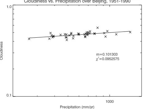
Fig. 1. Power law plot of rainfall and cloudiness over Beijing,
China, 1951–1990. Data is from Wang et. al., 1993.
as soil moisture. However, because the size of the bare fractionad is not determined solely by the biota, including
other variables in the vegetation birth rate overdetermines the model. In such a case, trees and grasses may not simultane-ously exist in steady state. We therefore elect to retain a birth rate dependent only on temperature.
2.4 Hydrological cycle
Water vapor is the largest greenhouse gas in the atmosphere. Therefore, the distribution of water in the atmosphere is im-portant for specification of radiative effects like cloud re-flectivity and greenhouse forcing. Functional relationships between surface water vapor characteristics and column in-tegrated water vapor have been tested with some success (Choudhoury, 1996). We therefore choose to keep track of a given region’s mean precipitable water, denotedwi, as a
sim-ple measure of region mean atmospheric water vapor. Mass balance gives
˙
wi =Ei −Pi+Fwi+Kwi (14)
whereEi is evaporation, Pi is precipitation,Fwi represents
the interregional atmospheric moisture transport, and Kwi
is the DAF adjustment for precipitable water. We use the Magnus-Tetens formulae for estimating thermodynamic vari-ables at saturation. Using the formula for saturation den-sityρs(T )for water vapor, we can calculate the saturation
mass per unit area for a vertical column of atmosphere us-ing a linear temperature profile with lapse rateγl=6.5 K/m
(Emanuel, 1994) with wsat(Ti)=
Z H
0
ρs(Ti+γlz)dz. (15)
A measure of the total relative humidity for a column can now be writtenri=wi/wsat(Ti).
Precipitation Pi is, of course, difficult to represent in a
0-D model. Convective rainfall is highly variable in both
space and time, and to accurately represent this requires a very sophisticated parameterization. We elect, therefore, to simply view precipitation as the mechanism by which the at-mosphere sheds excess water. As such, we leave a convec-tion parameterizaconvec-tion for the future and keep track of only annual mean rainfall, which has units of mass over time. The timescale should depend inversely upon local saturation, since a highly saturated atmosphere will rain more quickly than an unsaturated one. We therefore write
Pi =f0wi =(f rip)wi, (16)
after the parameterization used by Paul (1996), which devel-oped annual rainfall proportional to precipitable water, but with an additional power law dependence on column relative humidity. Mean annual regional cloudiness correlates loga-rithmically to precipitation (Fig. 1), so we take the regional cloud area fraction to be
aci =acoPiα. (17)
The empirical parametersf,p,aco, andαare to be
deter-mined from data.
Cloud albedoAci is a sensitive function of cloud height
(Hobbs and Deepak, 1981), and we assume that clouds form at a constant temperatureTcacross our model. A linear
pro-file for temperature, which we have already assumed for sat-uration, means thatHc(Ti)=(Ti−Tc)/γland
Aci(Ti)=Aco+κHc(Ti). (18)
HereTcis the cloud top temperature from Eq. (3), γ1l is the
linear slope for cloud height, andAcois the cloud albedo for
clouds at the surface. The linear response of cloud albedo to cloud height,κ, is an empirical parameter to be determined from data.
To represent evaporation, we choose a Penman-Monteith resistance model of the form
Ei =
(Rin,i−Rout,i)φ (Ti)+ρacpa(esat(Ti)−ei)rh
(φ (Ti)rh+γh(rh+rsi))Lv
, (19) where ρa is the density of the ambient air, cpa is the heat
capacity of the ambient air, rh is the hydrodynamic
re-sistance of bare soil, γh is the “psychrometer constant”,
and Lv is the latent heat of vaporization of liquid water.
φ (Ti) is an estimate of the derivative of the saturation
va-por pressureesat(Ti)close to the ground (Monteith, 1981),
ei=eo[ln(mwi)+Tc]ex is the vapor pressure determined from
the column integrated moisture (Emanuel, 1994), andrsiis
the stomatal resistance of the region’s biota. Stomatal resis-tance is a function of many things, most sensitively ambient carbon dioxide concentrations; but also intensity of sunlight, ambient temperature, and ambient relative humidity. Since carbon dioxide is fixed in this version of the model, in veg-etated regions we take resistance to be a function of relative humidity
settingh1=.004 m/s andh2=.096 m/s for consistency with the Ball-Berry model of stomatal conductance (Ball et al., 1987; Pleim, 1999). In non-vegetated regions,rsi=0.
The greenhouse forcing,ν, is taken to be a linear function of moisture. Here
ν=νc+νwmwi, (21)
withνcthe (constant) carbon forcing andνwthe absorptivity
of water across the visible and thermal spectra. Both param-eters remain to be estimated from data.
Soil moisture is also an important variable to track, since its distribution determines, to a large extent, the ability of vegetation to survive. Mass balance for the soil gives us ρwdsoils˙wi =(Pi−Ei+Fsi+Ksi), (22)
for si the soil water content in soil dsoil deep; ρw is the
density of water. We chooseFsi=Ds(s¯−si), andKsi
anal-ogously toKT i. Therefore, we take the death rate for biota
to be a quadratic function ofsi, the simplest function that is
zero at both saturation and drought.
We will assume for the purposes of this model that all in-terregional atmospheric transports occur through bulk move-ment of air, and thus through atmospheric circulation pat-terns. Then moisture transports in the atmosphere will follow the movement of heat, and they should reduce when there are smaller quantities of water in the atmosphere. We therefore makeFwi proportional toFT i and the ratio of global mean
precipitable water w¯ to the mean precipitable water at the current luminosity,w¯ |L=1.0. This assumption yields Fwi = [Dm(
¯
w
¯
w|L=1.0)]FT i, (23)
in whichDmis a constant determined by matching moisture
content over the model ice caps to present day polar values withw¯= ¯w|L=1.0. The value forw¯ |L=1.0can be found from Peixoto and Oort (1992) to be about 25.5 kg/m2.
2.5 Oceans
Oceans may be represented by a dynamic area fraction, with birth rate proportional to precipitation and runoff, and with death rate proportional to evaporation. Thus,
˙
ao=(ao[Po−Eo+Fso] +aabl µice)/Mo (24)
whereµiceis melt from the ablation zone of the polar caps
andMois the mass of a column of ocean water. We assume
a constant mean ocean depth for simplicity. Although the actual adjustment of the ocean fraction is small due to the large value of the constantMo, the effect of small changes
inao on the hydrological cycle in the rest of the model is
potentially significant.
The presence of the soil moisture convergence termFso,
included to capture the effects of runoff from land processes, requires the specification of a preferred soil moisture for the ocean, since we can’t directly write down a sensible analog of soil moisture in the ocean. Then
Fso=Ds(s¯−so), (25)
withsoa constant to be determined.
2.6 Ice caps
Ice caps can also be represented as a dynamic area frac-tion, but the DAF must be divided into two regions, an ab-lation zone and an accumuab-lation zone. The division between these zones will be made by mean annual temperature, since annual snowmelt in the polar regions is principally deter-mined by temperature and not by solar radiation (Bowman, 1982). We therefore construct a line of freezingθf rz, inside
of which ice sheets tend to grow and outside of which they ablate. The ice sheet poleward ofθf rz, where no significant
snowmelt occurs, will be known as the “accumulation zone”; whereas the ice sheet towards the equator fromθf rz will be
referred to as the “ablation zone”. This parameterization is constructed after the model discussed in Ghil and Childress (1987).
The freezing line is demarcated by a mean annual tem-perature equal to an effective freezing temtem-perature,Tf e,
dis-cussed below. θf rz may then be determined from the global
radiative balance by noting that the solar constant varies si-nusoidally with co-latitude, and may be reasonably approxi-mated by a square root for easy invertability. If we approx-imate the solar luminositySθ=S(Aθ+Bθ
√
(θ )), we can de-termine a co-latitudeθat which a given steady-state temper-atureTθwill occur by using a steady state assumption on (1),
such that
θ= [(Rin(wθ, Tθ)+FT ,θ)/Rout(wθ, Tθ)−Aθ]2/Bθ2. (26)
Herewθ is the local atmospheric moisture at temperatureTθ,
which can be found through a steady state assumption on a mass balance Eq. (14). Note thatKw,θ=0 becausewθ is
associated with a region of zero area.
The fractional area of a sphere that lies within a given co-latitude θ0 is (1−cosθ0)/2. If we assume north-south symmetry, this is multiplied by a factor of two such that the fractional area of a globe with an annual mean temperature lower thanTθisaθ=1−cosθ. Hence, the accumulation zone
has areaaacc=1−cosθf rz, θf rz is the co-latitude at which
snowmelt for the year is zero, and the ablation zone has area aabl=ai−aacc.
Under the DAF formalism, the area of the ice sheet updates with different precipitation- and evaporation-dependent mass balance rates in each subregion so that
ai =aacc(Pacc−Eacc)/MI+aabl(Pabl−Eabl−Nabl)/M(27)I,
whereNablis a melt rate andMI is the mean mass of a
col-umn of ice. Note that this formulation assumes a square pro-file for the ice sheet for simplicity, though it is possible to as-sume other profiles, as well. Moisture and temperature vari-ables must be calculated for each subregion to close Pacc,
Eacc, Pabl, andEabl. These variables are computed from
their respective balances at the zonal center of each subre-gion.
DAF adjustment termsKH ibecome somewhat tricky over
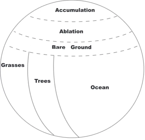
Fig. 2. Schematic of the layout of area fractions in this model. Ice caps are assumed to occur on the poles and to be symmetric. Dashed lines denote boundaries subject to dynamics, solid lines are fixed in time. Thus, all area fractions expand and contract into the bare ground region, except for the accumulation zone on the ice cap, which is surrounded by an ablation zone.
other regions expand into (see Fig. 2). Also, the ablation zone expands into both the accumulation zone and the bare land fraction. The fact that the ablation zone has two regions of expansion means it is necessary to specify in which direction the ablation zone has increased or decreased. Such a spec-ification, though somewhat more complex than the DAFM behavior exhibited by the other regions, is not conceptually difficult. It simply relies on determining the growth of the ice sheet as a whole andθf rz, then deductively specifying
growth of the component parts. However, the analytical treat-ment is messy and not particularly illuminating physically, so we will not discuss it here, other than to note that the two-region expansion is accounted for in the model. This two-region expansion is the basis for developing a DAFM in higher dimensions, where one obtains a dynamically adjust-ing grid.
Over ice caps, snowmelt Nabl must also be computed.
Energy balance models of the ice sheets (Bowman, 1982; Sandberg and Oerlemans, 1983; Paul, 1996) parameterize monthly snowmelt linearly in terms of monthly tempera-tureTmasNm(Tm)=550+1100(Tm−Tf)kg/yr withTf the
freezing point temperature 273.15 K.Tm, of course, does not
scale directly to an annual mean temperature, since the vari-ation of monthly mean temperatures is substantial in the arc-tic regions. To reconcile this parameterization to an annual mean temperature, it is necessary to replaceTf with an
ef-fective annual freezing temperature,Tf esuch that
Nabl =550+1100(Tabl−Tf e) kg/m2yr. (28)
Tf e is tuned to yield an ice-cap coverage of 2.9% since the
major land ice sheets on earth, Greenland and Antarctica, cover approximately that much of earth’s surface area.
3 Feedbacks
A model of this level of complexity contains many nonlinear processes, and as such it may be useful to enumerate feed-backs that have been included. For this purpose, we rewrite Eqs. (1) and (14) as
cpT˙i =SLA0i+σ νiTi4+σ aci[(1−νi)Ti4−T
4
c]
−SLA0iaciAci−σ Ti4
+FT i+KT i (29)
the expanded local heat update equation, and
˙
wi =Ei(wi, Ti)−f wi(1+p)wsat,i(Ti)−p+Fwi+Kwi(30),
the equation for local moisture update with precipitation ex-panded. The effect of each term in these equations is more clear when expanded, since positive feedbacks are sented by those terms added and negative ones are repre-sented by those subtracted.
The most obvious feedback is that between temperature and the blackbody term, the 5th term in (29), since it is un-coupled to other model variables. As local temperatureTi
in-creases, the amount of longwave radiation released from the atmosphere increases, evidently asTi4. This powerful nega-tive feedback provides a temperature bound for the climate system.
However, an increase in a local temperature also leads to increases in several diagnostic model variables. Both evap-oration Ei (19) and precipitation Pi (16) are increased, as
is seen in more complex models (Houghton et al., 20051). Sincemsat,iin the denominator ofPi is exponential in
tem-perature, the saturation point of the atmosphere increases, so mwiincreases as well.
The greyness factorνi (21) therefore increases, as does
cloud area as a function of the precipitation and cloud albedo as a direct function of temperature (see Eqs. 17 and 18). νi
appears in (29) coupled to temperature in the 2nd term, creat-ing a powerful positive feedback well known as the “Green-house” feedback.
Cloud fractionaciappears in the 3rd and 4th terms of (29).
Its effect in the 4th term is clearly that of a negative feedback, since it is coupled to the cloud albedo which also increases with temperature. This is commonly known as the shortwave cloud feedback. The effect of clouds on the 3rd term is more complex; for values of the cloud top temperature
Tc< (1−νi)1/4Ti (31)
1Houghton, J., Filho, L. M., Callender, B., Harris, N.,
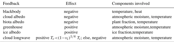
Table 1. Major feedbacks included in the full model.
Feedback Effect Components involved blackbody negative temperature, heat
cloud albedo negative atmospheric moisture, temperature biota albedo negative plant fraction, temperature greenhouse positive atmospheric moisture,temperature ice albedo positive ice fraction,temperature
cloud longwave positiveTc<(1−νi)1/4Ti; else, negative atmospheric moisture, temperature
this feedback will be positive, but forTc>(1−νi)1/4 Ti this
feedback is negative! That is, for high values of the grey-ness factor in this model, the effect of clouds in the longwave can actually be to cool the planet, an interesting feedback to be sure. However, it must be noted that such a situation is not physically realistic, since heat must first escape from the greenhouse gases below the clouds in order to reach the clouds and the model does not account for this. The possibil-ity of such a feedback is thus an artifact of our assumption of a constant cloud top temperature. We can view relation (31) as providing an upper bound for estimation of the parameter Tcin the model.
There is an ice-albedo feedback in the model, a positive feedback produced by the high reflective capabilities of polar ice. The accumulation angleθ(26) increases as a function of FT ,θ, which increases asT decreases. Thus colder
tempera-tures lead to a larger accumulation of ice, which reflects more heat.
Other feedbacks come from the surface processes in the model. From Eq. (11) withβ(Ti)expanded andγ (si)=γo+
γ0(si−sopt)2,
˙
ai =aiad−aiadk(Ti−Topt)2−aiγ (32)
The second term in this equation is a biota albedo feedback, negative since it increases as the local temperature strays from the optimal.
Feedbacks with ocean fraction are negligible, since the percent change of the area of the ocean system is extremely small. Major feedbacks in the model are listed in Table 1.
4 Parameter Estimation
As with any model, the DAFM requires the specification of several parameters and we choose these to resemble an earth-like climate. As a general and consistent rule, model param-eters are selected to bring the system variables to approxi-mately match annual means on earth. However, the parame-terizations themselves are applied by linearly scaling the an-nual mean estimates to the time scale of model integration, 1/1000th of a year, and by varying them on that timescale.
Our representation of the hydrological cycle demands specification of a fallout frequency,f; the relative humid-ity exponentp for precipitation; a base cloudiness,aco; the
precipitation exponent for cloudiness, α; the surface tem-perature slope for cloud albedo,κ; the minimum albedo for clouds,Aco; the greenhouse greyness due to carbon,νc; the
water vapor slope for water vapor greyness,νw; the preferred
oceanic soil moisture,so; the coefficient for the linear
trans-port of atmospheric moisture,Dw; the coefficient for the
lin-ear transport of soil moisture,Ds; the snowmelt temperature,
Tf e; and the cloud top temperatureTc.
We use data taken over Beijing, China (Wang et al., 1993) to find our power law exponent,α=.1, indicating a weak de-pendence for cloudiness on precipitation (Fig. 1). Since the earth’s mean cloudiness at our current temperature is 49%, we can findacofrom the mean conditions. The mean surface
temperature of the earth is around 288.4 K, its mean precip-itable water is about 25.5 kg/m2, and its mean albedo is 30– 35% (Peixoto and Oort, 1992). The minimum cloud albedo Aco, generally associated with low-lying fog, we take to be
.05 to match the albedo of the ocean. For stability the model requiresκ≤1/60, and for largerκthe clouds become increas-ingly more capable of adjusting albedo to block solar input; thus we takeκ to be its minimum possible value to prevent excessive bias towards homeostatic behavior in the hydro-logical cycle. Then, from the earth’s mean albedo, we can determine the cloud top temperatureTc.
Ice sheets cover 2.9% of the earth’s surface, which allows us to determine the annual melting temperature Tf e. The
precipitation exponentp, representing the power law depen-dence of precipitation frequency on column humidity, we de-termine by matching the frequency found from data in the ice cap model of Paul (1996) at earth-like conditions in our parameterization. We can now determine the frequency co-efficientf from the mean column moisture on earth.
The moisture transport coefficient we assume to be con-stant over the globe by construction; its value can be esti-mated from the polar moisture transport listed in Peixoto and Oort (1992). For simplicity, we useDw=Ds, dividing
mois-ture flux evenly between atmosphere and land. Model behav-ior is relatively insensitive to variations in this parameter in the neighborhood of its estimated value.
The carbon greynessνcis tuned to represent about 5% of
the greenhouse forcing. For a soil composed of 10% sand and 10% clay, saturation occurs atsi≈.45 and drought forsi≈.1
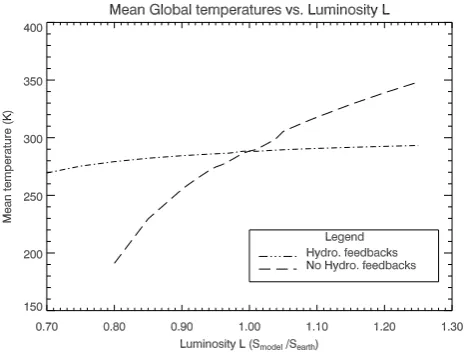
Fig. 3. Comparison of global mean temperatureT vs. luminosity
Lin a DAFM integration with fixed hydrological cycle to a DAFM with a dynamic hydrological cycle. Biota is dynamic and identi-cally forced in both plots. The hydrological cycle in the full DAFM produces an exceptionally strong stabilizing effect.
Taking a conservative estimate of the carbon greenhouse greyness, we can determineνw finally from the earth’s mean
temperature. Values of parameters used in our model runs for this analysis are listed in Tables 2 and 3.
5 Analysis
We perform two numerical experiments to emphasize the ef-fects of feedbacks between various components of the hydro-logical cycle on the global mean temperature of the model. In the first experiment, we compare runs of the fully coupled model with runs of a reduced model implementing only static hydrological variables over a range of solar luminositiesL.
In the second experiment, we modify theTopt parameter,
the uniform optimal temperature for seedling growth of both trees and grasses in the model. In the real ECS, this parame-ter may vary from species to species, and is not well known in general, so modifying the parameter serves two purposes: 1., to test model sensitivity to an unknown value; and 2., to show the range of control vegetation can have over surface temper-atures through changing evaporative properties and albedo.
As a basis for comparison in both experiments, we run the model to a steady state for earthlike conditions, as de-fined by a modern solar luminosity (L=1), a mean temper-ature near 288.5 K, mean precipitable water near 25.5 K, an ice cap fraction near 3%, cloudiness near 50%, realistic tem-peratures and precipitation near the poles, and approximately equal coverage for our two plant species.
5.1 Comparison to a fixed hydrological cycle varyingL The intent of this experiment is to establish a qualitative idea of the combined effects of various feedbacks between the hy-drological cycle and the heat balance on a planet like earth.
As such, we first compile data from a set of runs of the full model with solar luminosities ranging from 70% of present day insolation to 130%. In what follows, we shall refer to this set with the label(L).
For the second set of runs, labelled8(L), we fix all vari-ables associated with the hydrological cycle in the model, in-cluding regional cloudiness, regional cloud albedo, ice frac-tion, regional precipitable water, ocean fracfrac-tion, regional pre-cipitation, and regional evaporation, to the values obtained in the earthlike run,(L=1). Like(L), this data set is obtained by varyingL. Vegetation fractions and energy balances are the only climate components in8(L)allowed to respond to changes in insolation.
The contrast between the surface temperature values in the full model and those in that without water feedbacks is striking (Fig. 3). Changes in the global mean temperature in (L)are substantially smaller than they are in8(L), indicat-ing that an active hydrological cycle represents a tremendous net negative feedback for all values ofL. This result is par-ticularly interesting in light of the fact that two very strong and extremely important positive hydrological feedbacks are present in(L)but not in8(L), namely the ice-albedo and hydrological greenhouse feedbacks.
Since these are well-known to be positive feedbacks, other hydrological quantities in the radiative balance must be re-sponsible for this behavior. The only ones remaining are the nonphysical longwave cloudiness effect and the shortwave cloud albedo effect, which represent two possible mecha-nisms for a stabilizing effect. The first is due to an increase of both cloud area and cloud albedo in the shortwave term with increasing temperatures, and the second is due to the increased absorption and reemission of longwave radiation from the surface in the presence of more clouds. We would like to show that the latter is not the cause of this behavior, since we have discussed earlier that it is not physically rele-vant.
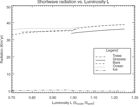
In Fig. 4 we plot the incoming shortwave radiation at the model’s surface over the five regional surface types. The im-portant feature in this plot is that the surfacial insolation on three of the four upper regional curves vary from their means on the order of 5% or less over the entire range of values of Ltested. The only exceptions are the region of bare ground, which varies on the order of 7%, and the ice cap, which cov-ers a very small fraction of the surface. This range ofL repre-sents a variation of 30% from its mean, so the behavior of the shortwave to solar forcing is extremely stable. It should also be noted that the slopes of these lines are generally decreas-ing withL. From Eq. (1) and the fact that the model resides at steady state, we can loosely approximate this behavior as a constant. Then we can write
Rin,i =Rout,i−FT i, (33)
Table 2. Parameters used in DAFM model runs.
parameter value meaning source
S 1.07e10 J/m2yr incident solar output Peixoto and Oort (1992)
sf1 .5 lat. temp. profile intercept Peixoto and Oort (1992) sf2 .6 l. temp slope w/
√
θ Peixoto and Oort (1992)
cpl 1.8e9 J/K m2 earth heat capacity calculated
Dw 1000. kg/m2/yr moisture transport (atmo) Peixoto and Oort (1992) from polar flux at 70N
BI 550. kg/yr base melting rate Bowman (1982)
ρw 1000 kg/m3 density of liquid water Peixoto and Oort (1992)
ds 1 m soil depth avg. root depth Salisbury and Ross (1992)
νc .217 carbon greyness contribution arbitrary, less than water
νw .0157 water greyness contribution per kg tuned for mean temperature
W slope 1.6 dewpoint slope with atm moisture Hobbs and Deepak (1981)
SAc 60 m−1 cloud albedo slope with height set for stability
Aco .05 base cloud albedo set to match oceans
A0b .85 tree co-albedo McGuffie and Henderson-Sellers (1997)
A0w .75 grass co-albedo McGuffie and Henderson-Sellers (1997)
A0d .8 bare land co-albedo McGuffie and Henderson-Sellers (1997)
A0o .9 ocean co-albedo McGuffie and Henderson-Sellers (1997)
A0acc .2 accumulation co-albedo McGuffie and Henderson-Sellers (1997)
A0abl .6 ablation co-albedo McGuffie and Henderson-Sellers (1997)
Table 3. Parameters used in DAFM model runs, cont’d.
parameter value meaning source
DT 1.3e8 J/m2yr heat transport (atmo) Budyko (1969)
k .003625 plant death exponent Watson and Lovelock (1983)
lapse .0065 atmos. temperature lapse rate Peixoto and Oort (1992)
σ 1.79 J/K4yr m2 Stefan-Boltzmann blackbody const Peixoto and Oort (1992)
T opt 286.23 K optimal growth temperature set for even occupation
Tf e 269.3 K annual temp for ice accumulation set to match ice fraction
α .1 rainfall-cloudiness exponent Wang et al. (1993)
ca 1006 J/K kg heat capacity of air Morton (1983)
h1 10 base hydrodynamic resistance set - small range of res. h2 90 hyd. res. slope with humidity (from 10 yr/m2to 100) Lf .3337e6 latent heat of freezing (water) Peixoto and Oort (1992)
Ls 2.834e6 latent heat of sublimation Peixoto and Oort (1992)
Lv 2.46e6 latent heat of vaporization Peixoto and Oort (1992)
mice 560 000 kg/m2 column mass of ice Peixoto and Oort (1992)
moo 3 800 000 kg/m2 column mass of ocean Peixoto and Oort (1992)
prexp .1 exponent for precip. with hum. Paul (1996)
πc .68 psychrometer constant Morton (1983)
rh 1.27e−6 s/m2 resistance to sensible heat Monteith (1981)
ρ .87 kg/m3 density of air Morton (1983)
ρi 800 kg/m3 density of ice Peixoto and Oort (1992)
terms,
X
i
aiσ (1−aci)(1−νi)Ti4=
X
i
[Ri−σ aiaciTc4]. (34)
Ifaci= ¯ac+i,νi= ¯ν+δi, andTi= ¯T+τi, then we can
approx-imate the above as σ (1− ¯ac)(1− ¯ν)T¯4[1−
P
iaii
1− ¯ac −
P
iaiδi
1− ¯ν +
4P
iaiτi
¯
T ] (35)
≈P
i[Ri−σ aiaciTc4], (36)
whence it is a simple matter to show that the three sums in the brackets are small. Thus, withR¯=P
iaiRi,
¯
T4≈ [ ¯R−σa¯
cTc4]/σ (1− ¯ac)(1− ¯ν) (37)
= ¯
R σ[
1− ¯ac(σ Tc4/R)¯
1− ¯ac
][ 1
1− ¯ν]. (38)
Fig. 4. Shortwave radiation at the surface by region for model runs with fully coupled water,(L). Variations in the shortwave forcing that reaches the surface are typically very small, despite a substantial change in the insolation at the top of the atmosphere.
non-physical negative feedback between cloud fraction and heat balance in the longwave (note that it is both physical and positive if condition (31) is met), and the third expresses the positive feedback inherent in the greenhouse effect.
We can now contrast the behavior of this equation in(L) and8(L)to see that it is the behavior of clouds in the short-wave band, expressed by the first factor in (38), that most supports the stability. For the fixed-water set 8(L), nei-thera¯cnorν¯ change at all; all changes inT¯4, therefore, are
caused by changes inR¯, which is linearly dependent onL. For(L), on the other hand,R¯ is nearly fixed, as shown in
Fig. 4.a¯cincreases with increasing temperature for(L), and
sinceσ Tc4/R<1, the second factor in (38) is also increas-¯ ing with increasing temperature (though it is slowed by the longwave negative feedback with cloud fraction).ν¯increases fairly rapidly, and so the third factor in (38) is the source of the most warming in(L). Thus, the second two factors in (L)drive the warming; and indeed, warm the model more than their counterparts in8(L) (which do not increase at all). Since the first factor increases very slowly for(L), it is clearly the source of the extraordinary stability.
5.2 The Effect of varyingTopt on surface temperatures
TheTopt parameter is difficult to estimate from data,
espe-cially considering that it probably varies relatively widely over species adapted to different climatic zones. However, it plays a relatively critical role, as it determines the range of temperatures over which the two species state (simultaneous trees and grasses) can exist.
In our DAFM, Topt is taken to be uniform among trees
and grasses, for simplicity. For the first experiments above, it was tuned to allow both species to occupy equal area frac-tions. Determining the sensitivity of our model to this param-eter gives not only an idea of the range of error associated in
quantitatively applying results from our model to earth, but also a way to demonstrate the full extent of the biota’s control over its environment.
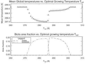
We vary Topt over a wide range of temperatures on the
interval [260,310]K and run the DAFM at earthlike con-ditions, using the (L=1) run from the previous test as initial conditions. The results are shown in Fig. 5. The plot breaks into five regions: one two-species region, two single-species regions, and two regions without biota. The two “dead” regions, on the intervalsT¯ ∈ [260,271]K and
¯
T ∈ [302,310]K, are at the same fixed temperature repre-senting the global mean dominated by ocean and desert.
The three “live” regions may be characterized by species dominance. The left hand region, in which the mean tem-perature T¯ is warmer than Topt, is dominated by the high
albedo grasses. HereT¯ is steadily reduced with increasing Topt as grasses become capable of covering a greater
frac-tion of the surface. The right hand region is dominated by the low-albedo trees, since T¯ is cooler than Topt. In this
region,T¯ also reduces with increasingTopt as trees are
in-creasingly less capable of covering the surface. The central region of the plot, in which both species share dominance of the planet, shows high sensitivity toTopt, as competition
between trees and grasses adjusts the global mean tempera-ture by more than 1 K. This suggests a surprising degree of control over the mean planetary temperature, as does the fact that the existence of trees and grasses in various configura-tions appears capable of adjustingT¯ by about 1.6 K.
6 Conclusion
With our simple hydrological DAFM, we have performed two numerical experiments to investigate the effects of cou-pling the hydrosphere and the biosphere on the global mean temperature of an earth-like planet.
Fig. 5. The effect of varying the optimal growth temperatureTopt on the global mean temperatureT. The temperature to the left and right of the upper plot is the temperature of a dead planet with no biota. Rapid changes in the center of the plot are due to nonlinear competition as the two species (trees and grasses) respond sensitively to changes inTopt.
to the surface of the earth, and so their effect on the short-wave radiative term is to reflect away a greater quantity of the sun’s input. This, of course, must be viewed as a cooling effect. Clouds are also efficient absorbers of longwave radi-ation and form at low temperatures such that the blackbody radiation they produce is much lower than that produced at the ground. This latter effect dictates that clouds also create a warming effect in the longwave term. While hardly con-clusive, the results from our model indicate that this effect is dominated by the relative constancy of the shortwave term, a behavior associated with the cloud albedo feedback.
It is possible that our choice for the cloud albedo slopeκ has affected the qualitative results of this experiment. We have used the minimum value available to us in the present configuration to reduce such an effect. However, we will test this possibility in a future paper. Our parameterizations for the longwave terms that could have affected results include our representation of the greenhouse effect; our assumption of fixed cloud top temperatures Tc; and our choice,
deter-mined as it was by other model parameters and variables, for the cloud top temperatureTc=270 K. An increased
car-bon greenhouse effectνcrelative to water vapor would lower
the cloud longwave term, while leaving the ground long-wave term approximately the same; this change would also not qualitatively affect results, since in this model carbon is treated as a static parameter. Changing cloud top tempera-turesTcwould have exactly the same effect.
It is possible that removing the assumption of constant cloud top temperatures in our model could qualitatively change the outcome of our model runs, and it is possible that
allowing carbon to dynamically adjust to climatic changes could do so as well. However, such a situation would re-quire very strong positive feedbacks in the carbon cycle or the cloud top temperatures. In a future paper, we intend to examine results from runs with both of these assumptions re-moved.
It is interesting to note that these model runs produced no “iceball” effect, even at tremendously low luminosities L. We have also tested much lower values of the heat transport parameterDT and found only modest changes in the size of
the ice sheet. This phenomenon is even more interesting in light of the fact that we used the linear Budyko parameter-izaton for heat transport, which was cited as a cause of the iceball effect in his seminal paper (Budyko, 1969; Sellers, 1969). It is possible that the presence of the feedbacks in our model’s active hydrological cycle or its biota has prevented this from occurring. However, at present such a conclusion would be speculative, since we have not tested the system sufficiently thoroughly to determine why the ice caps do not grow to cover the system.
In the second experiment, we changed growing character-istics associated with the biota by adjusting the optimal tem-perature for seedling growth,Topt. We found that the range
It remains to add dynamic carbon feedbacks to this model, like those studied in Svirezhev and von Bloh (1998). A future paper coupling the two cycles would certainly produce inter-esting results. It would likewise be interinter-esting to establish lo-cal heat capacities,cpi. In addition, more spatial dependency
should be added, as biota have different growing character-istics at different latitudes and the effect of landform loca-tion is suspected of playing some role in determining global climate. Using different optimal growing temperatures for trees and grasses might also allow us to include growth de-pendence on other model variables, such as soil moisture.
More generally, there is a great need in this and other mod-els to develop a rigorous framework for parameterizations, one that explicitly incorporates the basic issue of scale de-pendence and scale invariance in biophysical processes. For example, in this model and others (Pan, 1990), a Penman-Monteith equation has been used to represent evapotranspi-ration at relatively large spatial scales. However, Choudury (1999) found that the Penman-Monteith equation was not scale invariant across a very broad range of spatial scales tested in the biophysical model they studied. Such a re-sult reinforces that the Penman-Monteith equation is valid only for very specific scales and should not be directly ap-plied to larger ones. At present, the study of scaling trans-formations on biophysical parameterizations is in its infancy (e.g. Milne et al. (2002)). Thus the biophysical parameteriza-tions available to modelers at present are typically not scale-appropriate.
Finally, there is a need to establish model parameteriza-tions in all climate models consistent with some established set of basic physical principles. Unfortunately, there has been relatively little attention paid to how to elucidate such a set of principles in a system like Earth’s climate system, which is a highly nonlinear system far from equilibrium or steady state. For example, a promising candidate in this area is the Maximal Entropy Production (MEP) formalism developed by Paltridge (1975) and others (for an excellent review see Ozawa et al. (2003)). Only by establishing such a consis-tent theoretical framework will we be able to effectively de-velop parameterizations capable of representing higher-order moments as well as the means, or ensure consistency in our physical schemes and the results. In future DAFM models we intend to explore the development of parameterizations under a MEP formalism.
Acknowledgements. The first author would like to thank the
National Science Foundation (NSF) for its generous support under a Graduate Research Traineeship (GRT) grant awarded to the University of Colorado hydrology program, which made the development of this work possible as part of his PhD disserta-tion. He and the second author would also like to acknowledge NSF for its continued support as the work evolved under grants EAR-9903125 and EAR-0233676.The third author wishes to acknowledge NSF grant number ATM-0001476 in support of this research. All the three authors gratefully acknowledge the CIRES Innovative Research Program for its support of this research.
Edited by: B. Sivakumar Reviewed by: two referees
References
Ball, J., Woodrow, I., and Berry, J.: A model predicting stomatal conductance and its contribution to the control of photosynthesis under different environmental conditions, Progress in Photosyn-thesis Research, IV, 221–234, 1987.
Bowman, K.: Sensitivity of an annual mean diffusive energy bal-ance model with an ice sheet, J. Geophys. Res., 87, 9667–9674, 1982.
Boyce, W. and DiPrima, R.: Elementary differential equations and boundary value problems, 5th ed., Wiley, New York, 1992. Budyko, M.: The effect of solar radiation variations on the climate
of the Earth, Tellus, 5(9), 611–619, 1969.
Choudhoury, B.: Comparison of two models relating precipitable water to surface humidity using globally distributed radiosonde data over land surfaces, Int. J. Climatol., 16, 663–675, 1996. Choudury, B.: Evaluation of an empirical equation for annual
evap-oration using field observations and results from a biophysical model, J. Hydrol., 216, 99–110, 1999.
Claussen, M., Crucifix, M., Fichefet, T., Ganopolski, A., Goosse, H., Lohmann, G., Loutre, M.-F., Lunkeit, F., Mohkov, I., Mysak, L., Petoukhov, V., Stocker, T., Stone, P., Wang, Z., Weaver, A., and Weber, S.: Earth system models of intermediate complexity: Closing the gap in the spectrum of climate system models, Clim. Dyn., 18, 579–586, 2002.
Emanuel, K.: Atmospheric convection., Oxford Univ. Press, New York, 1994.
Ghil, M. and Childress, S.: Topics in geophysical fluid dynamics: Atmospheric dynamics, dynamo theory, and climate dynamics, Springer-Verlag, NY, 1987.
Harvey, L. and Schneider, S.: Sensitivity of internally generated cli-mate oscillations to ocean model formulation, in: Proceedings on the Symposium on Milankovitch and Climate, edited by: Berger, A., Imbrie, J., Hays, J., Kukla, S., and Saltzman, B., ASI, pp. 653–667, NATO, D. Reidel, Hingham, MA, 1987.
Hobbs, P. and Deepak, A.: Clouds: Their formation, optical prop-erties, and effects, Academic Press, NY, 1981.
Houghton, J., Filho, L. M., Callender, B., Harris, N., Kattenberg, A., and Maskell, K.: Contribution of working group I to the sec-ond assessment of the intergovenmental panel on climate change, in: IPCC Second Assessment – Climate Change 1995, MIT Press, Cambridge, MA, 1995.
Lovelock, J.: Gaia as seen through the atmosphere, Atmos. Envi-ron., 6, 579–580, 1972.
Lovelock, J. and Margulis, L.: Atmospheric homeostasis by and for the biosphere: the Gaia hypothesis, Tellus, 26, 1–10, 1974. McGuffie, K. and Henderson-Sellers, A.: A climate modeling
primer (Research and development in climate and climatology), J. Wiley and Sons, NY, 1997.
Milne, B., Gupta, V., and Restrepo, C.: A scale invariant coupling of plants, water, energy, and terrain, Ecoscience, 9(2), 191–199, 2002.
Monteith, J.: Evaporation and surface temperatures, Quarterly Jour-nal of the Royal Meteorological Society, 107, 1–27, 1981. Morton, F.: Operational estimates of areal evapotranspiration and
Nordstrom, K.: Simple models for use in Hydroclimatology, Ph.D. thesis, University of Colorado at Boulder, 2002.
Nordstrom, K., Gupta, V., and Chase, T.: Salvaging the Daisyworld parable under the Dynamic Area Fraction Framework, in: Scien-tists Debate Gaia: the next century, edited by: Miller, J., Boston, P., Schneider, S., and Crist, E., MIT Press, Cambridge, MA, 2004.
O’Brian, D. and Stephens, G.: Entropy and climate II: Simple mod-els, Quarterly Journal of the Royal Meteorological Society, 121, 1773–1796, 1995.
Ozawa, H., Ohmura, A., Lorenz, R., and Pujol, T.: The second law of thermodynamics and the global climate system: a review of the maximum entropy production principle, Rev. Geophys., 41(4), 1018, 2003.
Paltridge, G.: Global dynamics and climate – A system of minimum entropy exchange, Quart. J. Roy. Meteor. Soc., 101, 475–484, 1975.
Pan, H.-L.: A simple parameterization scheme of evapotranspi-ration over land for the NMC medium-range forecast model, Monthly Weather Review, 118, 2500–2512, 1990.
Paul, A.: A seasonal energy balance climate model for coupling to ice-sheet models, Ann. Glaciol., 23, 174–180, 1996.
Peixoto, J. and Oort, A.: Physics of climate, American Institue of Physics, NY, 1992.
Pleim, J.: Modeling stomatal response to atmospheric humidity, in Preprints of the 13th Symposium on Boundary Layers and Tur-bulence, January 10–15 1999 in Dallas, TX, American Meteoro-logical Society, Boston,MA, 1999.
Salisbury, F. and Ross, C.: Plant physiology (4th ed.), Wadsworth Publishing Co., Belmont, CA, 1992.
Sandberg, J. and Oerlemans, J.: Modelling of Pleistocene European ice sheets: The effect of upslope precipitation, Geologie en Mjin-bouw, 62, 267–273, 1983.
Sellers, W.: A global climatic model based on the energy balance of the Earth-atmosphere system, J. Appl. Meteorol., 8, 392–400, 1969.
Svirezhev, Y. M. and von Bloh, W.: Climate, vegetation, and global carbon cycle: the simplest zero-dimensional model, Ecological Modeling, 101, 79–95, 1998.
Wang, W., Zhang, Q., Easterling, D., and Karl, T.: Beijing cloudi-ness since 1875, J. Clim., 6, 1921–1927, 1993.
Watson, A. and Lovelock, J.: Biological homeostasis of the global environment: the parable of Daisyworld, Tellus, 35B, 284–289, 1983.