A practical scheme to introduce explicit tidal forcing into an OGCM

www.ocean-sci.net/9/1089/2013/ doi:10.5194/os-9-1089-2013

© Author(s) 2013. CC Attribution 3.0 License.

Ocean Science

A practical scheme to introduce explicit tidal forcing into an OGCM

K. Sakamoto, H. Tsujino, H. Nakano, M. Hirabara, and G. Yamanaka

Meteorological Research Institute, Nagamine, Tsukuba, Ibaraki 305-0052, Japan Correspondence to: K. Sakamoto ([email protected])

Received: 14 February 2013 – Published in Ocean Sci. Discuss.: 7 March 2013

Revised: 4 October 2013 – Accepted: 22 October 2013 – Published: 13 December 2013

Abstract. A practical scheme is proposed to explicitly intro-duce tides into ocean general circulation models (OGCM). In this scheme, barotropic linear response to the tidal forcing is calculated by the time differential equations modified for ocean tides, instead of the original barotropic equations of an OGCM. This allows for the usage of various parameteriza-tions specified for tides, such as the self-attraction/loading (SAL) effect and energy dissipation due to internal tides, without unintentional violation of the original dynamical bal-ances in an OGCM. Meanwhile, secondary nonlinear effects of tides, e.g., excitation of internal tides and advection by tidal currents, are fully represented within the framework of the original OGCM equations. That is, this scheme drives the OGCM by the barotropic linear tidal currents which are predicted progressively by a tuned tide model, instead of the equilibrium tide potential, without large additional numerical costs. We incorporated this scheme into Meteorological Re-search Institute Community Ocean Model and executed test experiments with a low-resolution global model. The results showed that the model can simulate both the non-tidal cir-culations and the tidal motion simultaneously. Owing to the usage of tidal parameterizations such as a SAL term, a root-mean-squared error in the tidal heights is found to be as small as 10.0 cm, which is comparable to that of elaborately tuned tide models. In addition, analysis of the speed and energy of the barotropic tidal currents is found to be consistent with that of past tide studies. The model also showed active ex-citement of internal tides and tidal mixing. In the future, the impacts of internal tides and tidal mixing should be exam-ined using a model with a finer resolution, since explicit and precise introduction of tides into an OGCM is a significant step toward the improvement of ocean models.

1 Introduction

Recent advances in theories of ocean general circulations and observations of deep seas have revealed that tides play a sig-nificant role in open oceans as well as in coastal areas. As a representative study, Munk and Wunsch (1998) suggested that vertical mixing in deep seas due to breaking of inter-nal tides is an important process in the global thermohaline circulations. This hypothesis is supported by the fact that a large part of the tidal energy is dissipated in deep seas (Eg-bert and Ray, 2001; St. Laurent and Garrett, 2002; Niwa and Hibiya, 2011). In addition, various studies reported that local strong tidal mixing affects the ocean circulations on a basin scale. For example, tidal mixing near the Kuril Islands plays an important role in the formation process of the water mass called the North Pacific Intermediate Water (Nakamura and Awaji, 2004; Osafune and Yasuda, 2006). Tidal mixing in the Arctic Shelf seas modifies the salinity budget through interaction with sea ice, and, as a result, the deep thermo-haline circulation in the North Atlantic (Postlethwaite et al., 2011). In a similar fashion, tidal mixing over the Antarctic shelves affects the formation process of Antarctic Bottom Water (Robertson, 2001a, b; Pereira et al., 2002). These stud-ies suggest an influence of tides on the general circulation.

1090 K. Sakamoto et al.: A practical scheme to introduce explicit tidal forcing into an OGCM

Discussion

P

ap

er

|

Discussion

P

ap

er

|

Discussion

P

ap

er

|

Discussion

P

ap

er

|

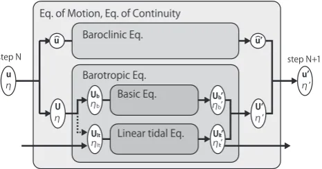
Fig. 1. A schematic view of the calculation procedure of the tide scheme. Fromuandηat the time step

N,u′andη′at the next stepN+ 1are calculated following the equations of motion and continuity. In the calculation process, the mode splitting technique splits the variables into the baroclinic constituent,

ˆ

u, and the barotropic one,Uandη, and then the tide scheme splits the latter into the basic compo-nent,Ubandηb, and the linear tidal component,Ultandηlt. Each component calculates time evolution

(uˆ′,Ub′, η′b,Ult′ andη′lt), and subsequently all of them are summed to obtainu′andη′. The dashed and

solid arrows which point toUltandηltmean that their time evolution are given almost independently

(see the main text).

36

Fig. 1. A schematic view of the calculation procedure of the tide

scheme. Fromuandηat the time stepN,u0andη0at the next step

N+1 are calculated following the equations of motion and

conti-nuity. In the calculation process, the mode splitting technique splits

the variables into the baroclinic constituent,uˆ, and the barotropic

one, U and η, and then the tide scheme splits the latter into

the basic component,Uband ηb, and the linear tidal component,

U_lt andηlt. Each individual component calculates time evolution

(uˆ0,U_b0, η_b0,U_lt0 andη_lt0), and subsequently all of the time evolution

values are summed to obtainu0andη0. The dashed and solid arrows

which point toUltandηlt indicate that their time evolution values

are given almost independently (see the main text).

The methodology of incorporating tides into OGCMs is classified into two types, i.e., an implicit one and an ex-plicit one. Models with the imex-plicit type use indirect pa-rameterizations about tidal effects rather than simulating tides themselves, in order to avoid drastically changing the OGCM framework. A typical parameterization adopted by various recent OGCMs is a mixing enhancement in deep seas and coastal areas (e.g., St. Laurent and Garrett, 2002). Lee et al. (2006) reported that this kind of parameterization contributes to good representation of the salinity distribution in the North Atlantic. As another indirect parameterization, Bessiéres et al. (2008) proposed an implicit parameterization for the tidal residual currents.

The explicit type introduces the tidal dynamics into free-surface OGCMs directly; i.e., through introduction of tidal forcing in the momentum equations. Though this type needs large computer resources and modification of a part of the OGCM framework, some achievements have been al-ready reported. For example, Schiller and Fiedler (2007) improved model representation of water transport and mix-ing in the Indonesian Through Flow region and Australian shelves. Müller et al. (2010) reported improvement in mod-eling of the pathway of the North Atlantic Current and water-modification processes in the North Atlantic. In addition, Ar-bic et al. (2010) discussed a possibility that explicit incor-poration of tides into an eddy-resolving OGCM may lead to drastic improvement in the representation of various ocean processes – such as interaction between meso-scale eddies and tides, form drag on the sea mounts, and the excite-ment and propagation of internal tides – in realistic

three-dimensional stratification. Development of an OGCM, which simultaneously simulates the time evolution of the tidal field and the non-tidal field (called the basic field hereafter), is now a frontier in ocean modeling.

By contrast, the modeling of tides themselves has been developed virtually independently of OGCMs, based on barotropic ocean models. Many modeling studies have shown that dynamics particular to tides need to be introduced into the model equations for accurate representation of tides (e.g., Matsumoto et al., 2000). A typical example is the self-attraction/loading (SAL) effect. This represents modification of the gravity field and elastic deformation of the bottom ground induced by movement of ocean water (Schwiderski, 1980). Due to the SAL effect, the pressure gradient term ac-companied by the tidal height gradient,−g∇η, is modified in the equation of barotropic motion as follows:

−g∇(η−ηSAL), (1)

whereηis the sea surface height (SSH) anomaly (m) andgis the gravitational acceleration (m s−2) (See Table 1 for vari-ables and constants in this paper). In order to represent the gravity change of the self-attraction and the loading effect – which is that the sea surface elevation induced by conver-gence of barotropic velocities is partially canceled by depres-sion of the bottom ground due to water weight – the elevation is subtracted byηSALin the calculation of the pressure

gradi-ent. Though various evaluations ofηSALhave been proposed,

a linear response is used as a first-order approximation,

ηSAL=(1−α)η, (2)

whereα is a constant between 0.88 and 0.95 (Matsumoto et al., 2000). Under this approximation of the SAL term, which has been traditionally referred to as the “scalar approx-imation” (Hendershott, 1972), the pressure gradient term

−g∇ηis modified to−gα∇η.

Another issue of tide modeling is energy dissipation of tides, such as energy transfer to internal tides and form drag by bottom topography on tidal currents. In general, as model resolution becomes finer, a model can represent more kinds of dissipation processes without parameterization. However, considering that internal tide processes cannot be reproduced sufficiently even in a model with a horizontal resolution of 10 km, which is considerably fine at present (e.g. Niwa and Hibiya, 2011), a parameterization specialized for dissipation is still necessary to represent tides with good accuracy (Jayne and St. Laurent, 2001; Arbic et al., 2004). Furthermore, var-ious parameterizations unusual for OGCMs have been pro-posed for tidal modeling, such as body tides, which are in-cluded here, and atmospheric tides. See Chapter 6 of Kantha and Clayson (2000) for a detailed description.

Table 1. Mathematical variables and constants in the main text and Appendix.

a the damping coefficient of Eq. (A10) (s−1)

b(suffix) the basic (nonlinear-tidal) components

BKE the volume-averaged kinetic energy of the barotropic currents (m2s−2)

Cd the bottom drag coefficient (dimensionless)

D the energy dissipation (Wm−2)

D a dissipation parameterization (m2s−2)

Dmodified dissipation modified for a tidal model (m2s−2)

f the Coriolis parameter (s−1)

F the horizontal gradient ofη0(dimensionless)

F+ the amplitude of the counterclockwise component ofF(dimensionless)

F− the amplitude of the clockwise component ofF(dimensionless)

Fw the surface freshwater flux (m s−1)

g the gravitational acceleration (m s−2)

H the water depth (m)

IB(suffix) the ideal basic components in Eq. (21)

IT(suffix) the ideal tidal components

k the upward vertical unit vector (dimensionless)

lt(suffix) the linear tidal components

P the tide energy flux (Wm−1)

R+ the amplitude of the counterclockwise component ofU(m2s−1)

R− the amplitude of the clockwise component ofU(m2s−1)

t time (s)

T temperature (C◦)

Tθ the horizontal veering of bottom friction (dimensionless)

U the vertically integrated transport vector (m2s−1)

W the energy supply of tides (Wm−2)

X residual terms (advection, wind stress, etc.) (m2s−2)

x the longitude coordinate (m)

y the latitude coordinate (m)

z the vertical coordinate (m)

α the scalar approximation constant of the SAL term (dimensionless)

β the constant of the body tide effect (dimensionless)

η the sea surface height anomaly (m)

η0 the equilibrium tidal potential (m)

ηSAL the SAL term (m)

ηt the tidal height (SSH anomaly from case NOTIDE) (m)

σ0 the potential density (kg m−3)

σ the tidal frequency (s−1)

τbtm the bottom friction (divided by standard density) (m2s−2)

proposed terms for tidal modeling are incorporated into the OGCM equations directly (Arbic et al., 2010). For example, the SAL term of Eq. (1) changes the geostrophic relation-ship between sea surface gradient and currents. Parameteri-zations for dissipation of tidal currents are not suited for the geostrophic currents in OGCMs either, since their time scales of change are so different from each other that their dissi-pation mechanisms are not the same. Therefore, we cannot simply replace the governing equations of OGCMs by those of tidal modeling. The two sets of the governing equations should be harmonized by some means in order to introduce tides into an OGCM.

1092 K. Sakamoto et al.: A practical scheme to introduce explicit tidal forcing into an OGCM

elaborated a method to prevent the parameterizations spe-cialized for tides from affecting the basic fields. Specifically, they defined the tidal currents as velocity deviations from a 25-hour running mean (which is calculated progressively in the model), and restricted the tidal dissipation parameteriza-tion to work on the tidal currents only. In addiparameteriza-tion, they de-fined the tidal height as the SSH deviation from the dynam-ical height (which is calculated every time step), and evalu-ated the SAL term so that the SAL would not contaminate the basic field (e.g., geostrophic currents). However, their method is expected to expend a substantial amount of numer-ical resources. Furthermore, it seems questionable that all of the SSH deviation is treated as tidal height.

As a solution to the aforementioned problem, we propose a new practical scheme to incorporate tides explicitly into OGCMs. This scheme is based on the recognition that the governing equations are different between the tidal and basic fields, and calculates their time evolutions separately. This approach is in contrast to traditional typical schemes such as that by Schiller (2004), in which the tidal and basic fields are given by the same governing equations.

First this paper will explain our scheme in detail. Next, model representations of tides by this scheme will be shown based on some test experiments of a global OGCM. Finally, tidal effects on the basic fields in the OGCM will be pre-sented briefly.

2 Scheme and model

2.1 Conventional scheme

Before presenting the new tide scheme, we will discuss the scheme of Schiller (2004) as a representative example of the traditional schemes in which the tidal forcing is incorporated directly into the governing equations. First, the original stan-dard expressions of the barotropic equations of motion and continuity are

∂U

∂t +fk×U= −g(η+H )∇η+D+τ

btm_{+X (3)}

∂η

∂t + ∇ ·U=Fw, (4)

wheret is the time (s),U the vertically integrated transport vector (m2s−1_{),f the Coriolis parameter (s}−1_{),k the}

up-ward vertical unit vector (dimensionless),Hthe water depth (m),Da dissipation parameterization (m2s−2),τbtmthe bot-tom friction (already divided by standard density) (m2s−2),

Xthe other residual terms including the vertically integrated advection and the wind stress (m2s−2), andFw the surface freshwater flux (m s−1). Introduction of tides means that the equilibrium tidal potential η0 and the SAL term ηSAL are

added, andDis changed to the dissipation parameterization

specialized for tides, which is indicated byDmodified, as

∂U

∂t +fk×U= −g(η+H )∇(η−βη0−ηSAL) (5)

+Dmodified+τbtm+X,

whereβrepresents the body tide effect (Schwiderski, 1980). If the scalar approximation for the SAL term, Eq. (2), is adopted, Eq. (6) becomes

∂U

∂t +fk×U= −g(η+H )∇(αη−βη0) (6)

+Dmodified+τbtm+X.

This is equivalent to a standard barotropic tidal model, e.g., the continuous ocean tide equations of Schwiderski (1980). In this traditional scheme, the time evolutions of U andη under the tidal forcing are obtained by solving Eqs. (4) and (6) (or (7)) underη0(x, y, t ), which is analytically calculated.

This scheme works well for modeling of tides without ba-sic circulation. However, in modeling of the tidal and baba-sic fields simultaneously, it induces the problem that the terms specialized for tides affect the basic fields unintentionally. In fact, Eq. (7) clearly shows that the SAL term changes the relationship between the sea surface gradient and the barotropic currents. The dissipation,Dmodified, also changes

the basic currents. Introduction of parameterizations speci-fied for tides results in violation of the dynamical balances in the basic fields.

2.2 New scheme

The violation of the dynamical balance in the basic fields arises from the fact that the barotropic equation of motion for tides, Eq. (6), is different from the OGCM standard equation for the basic fields, Eq. (3). Therefore, our new tide scheme calculates the tidal and basic fields by two different equations as explained below. The objective of our new scheme is to simultaneously achieve both accurate modeling of the tides and maintenance of the dynamical balances in the original OGCM.

The basis of the scheme is decomposition of the variables,

U,η,D andτbtmin the barotropic equations into the linear tidal component and the basic component,

U=Ub+Ult (7)

η=ηb+ηlt (8)

D=Db+Dlt (9)

τbtm=τ_bbtm+τ_ltbtm

. (10)

and so on). There are some difficulties posed by the decom-position of the variables, especiallyτbtm, and this decompo-sition is discussed in more detail later.

Each of the two components is calculated using its own governing equation. The linear tidal component is governed by the equations for tidal modeling; i.e., a modified Eq. (6) and the continuity equation:

∂Ult

∂t +fk×Ult= −g(η+H )∇(ηlt−βη0−ηSAL) (11)

+Dlt+τltbtm

∂ηlt

∂t + ∇ ·Ult=0. (12)

The basic component is governed by the standard OGCM equations, i.e., Eqs. (3) and (4).

∂Ub

∂t +fk×Ub= −g(η+H )∇ηb+Db+τ

btm

b +X (13) ∂ηb

∂t + ∇ ·Ub=Fw (14)

The numerical procedure to predict the two components by the equations above is schematically illustrated by Fig. 1. Generally in a free-surface OGCM, if one starts with velocity

uand SSHηat the time stepN, the velocity and SSH at the next step,N+1, are calculated using the equations of motion and continuity, and usually the barotropic and baroclinic con-stituents are predicted differently in the calculation (so called mode splitting, indicated byuˆ,Uandηin Fig. 1). The key to our new scheme is to further split the barotropic constituent into the basic and linear tidal components (Ub, ηb,Ult and ηlt), and to calculate the time evolution ofUlt andηlt sepa-rately fromUbandηb. The solid arrow connected toUlt and ηlt in Fig. 1 indicates this independent calculation, whereas the dashed arrow means thatUbandηbare given by subtrac-tion, i.e.,U−Ultandη−ηlt, respectively. That is, the three sets of the governing equations are calculated at each time step, and the three-dimensional velocity field at the next step is determined by their summation.

The linear terms in the barotropic equations, such as the Coriolis force and the Laplacian horizontal viscosity, can be split into the basic and linear tidal components natu-rally, while the nonlinear terms need to be treated more care-fully. In our scheme, all of the advection terms are incorpo-rated into the basic equations (Xin Eq. (13)), and the lin-ear tidal equations have no advection. Specifically, the tracer and momentum advections are calculated using the three-dimensional velocity field, given by the summation of all of their components (uin Fig. 1), and these sums are added to the basic equations. This is based on the assumption of the following scheme: the linear tidal component represents only the linear primary response to the tidal forcing, and the other secondary effects, such as tidal advection and internal tides, are represented by the basic component. Modification of the

tides due to interaction between tidal currents and basic fields is also represented by the basic equations as secondary oscil-lations with tidal frequencies (see Appendix for detail).

The wind stress (included inX) and the freshwater flux Fw are also left in the original OGCM equations, Eqs. (13) and (14). This is because the wind-induced circulations and the thermohaline circulations induced by these terms should be represented in the OGCM framework. If these terms were moved to the linear tidal equations, the dynamical balance would be violated due to tidal parameterizations such as the SAL term. In addition, as far as we know, it has not been re-ported that these terms change the primary response of the ocean to the tidal forcing. Nevertheless, various processes of secondary interaction between tides and basic fields have been reported, e.g., influence of tidal mixing on a thermoha-line circulation (Lee et al., 2006) and modification of internal tides induced by winds (Xing and Davies, 1997). These kinds of interaction processes are intended to be represented under the OGCM equations.

Decomposition of the bottom frictionτbtmshould be care-fully treated, since it is nonlinear, when expressed by a quadratic form as (Taylor, 1920; Weatherly et al., 1980)

τbtm= −CD

U

H+η

Tθ

U

H+η. (15)

The constantCD indicates a drag coefficient and the Tθ in-dicates a matrix representing horizontal veering,

Tθ=

cosθ−sinθ sinθ cosθ

, (16)

whereθ is the veer angle. (The unitτbtmis given in m2s−2_,

andCD and Tθ are dimensionless.) There are various ways to split Eq. (15) into the term for the basic barotropic equa-tion and that for the linear tidal equaequa-tion. For simplicity of the equations, we decided that a sum of the two components would be used for|U/(H+η)|(the coefficient part), but each component forU/(H+η)(the vector part) would be given by

τ_bbtm= −CD

Ub+Ult H+η

Tθ

Ub

H+η (17)

τ_ltbtm= −CD

Ub+Ult H+η

Tθ

Ult

H+η. (18)

1094 K. Sakamoto et al.: A practical scheme to introduce explicit tidal forcing into an OGCM

decomposition, we make the linear tidal equations, Eqs. (11) and (12), as simple as possible, in order to represent only the primary barotropic response to the tidal forcing.

Using our new scheme, we can avoid the violation of the dynamical balance in the basic field. To show this achieve-ment more clearly, we assume the SAL term has a linear form asηSAL∼(1−α)ηlt, and sum Eqs. (13) and (12) to find that

∂U

∂t +fk×U= −g(η+H )∇(ηb+αηlt−βη0) (19)

+Db+Dlt+τbbtm+τ

btm

lt +X.

This equation for motion is clearly different from the con-ventional scheme, Eq. (7). The SAL effect (α) works onηlt only, the body tide effect works on the equilibrium tide only, and the expressions for dissipation and bottom friction for tides (Dlt andτ_ltbtm) are different from the basic field (Db andτ_bbtm). As a result, when tides are omitted (i.e.,η0≡0),

Ult, ηlt,Dltandτ_ltbtmare permanently zero in Eqs. (11), (12) and (18), so that Eq. (19) becomes identical to the original barotropic equation, Eq. (3). Thus, the introduction of our tide scheme, in contrast to conventional tide schemes, does not modify the basic equations.

From the point of view of tidal modeling, our scheme en-ables us to tune the parameterizations of tides independently of the dynamical balance in the basic field. The value ofα, the formulation ofτ_ltbtmand the parameterization ofDlt can be selected independently.

To clarify the base of the new scheme, the meaning of “the linear tidal component” is noted again here. Strictly speak-ing, a part of the basic component ofηis used in Eqs. (11) and (12) so the linear tidal component is not strictly inde-pendent of the basic component. However, the linear tidal component is treated separately from the basic component. In other words, the scheme calculates the linear tidal currents under the equilibrium tidal potential progressively, and uses it as a model forcing, instead of introducing the potential to the model directly. That is, the linear tidal component can be referred to as an external forcing for the model, rather than the tidal field reproduced in the model. To see the tidal field precisely, secondary oscillations with tidal frequencies in the basic field need to be taken into account, as explained in the Appendix.

In closing this subsection, the practical approximation used by our new scheme is compared with the scheme of Arbic et al. (2010) in detail. The first principle of our new scheme is that the different sets of the governing equa-tions should be applied to the tidal component and the non-tidal component separately, in order to introduce tides into OGCMs realistically. To do so, we have to carry out de-composition of the two components in an OGCM. In an ideal scheme, the tidal component would represent all of the barotropic motions which oscillate with tidal frequencies and have the spatial structures corresponding to the tidal forc-ing, while the non-tidal component would represent all of the other motions. Hereafter, we call these components “the ideal

tidal component” and “the ideal basic component”, respec-tively. Under such an ideal decomposition, the barotropic equation comparable to Eq. (19) becomes

∂U

∂t +fk×U= −g(η+H )∇(ηIB+αηIT−βη0) (20)

+DIB+DIT+τIBbtm+τ btm

IT +XIB+XIT,

where the variables with the “IB” and “IT” subscripts indi-cate the ideal basic component and the ideal tidal component, respectively. However, it is virtually impossible to extract the ideal tidal component (i.e., all of the motions with tidal fre-quencies and with spatial patterns corresponding to the tidal forcing), from the changing model results. A certain approx-imation is necessary for the decomposition.

In the scheme of Arbic et al. (2010), the decomposition is executed in a straightforward manner. Arbic et al. (2010) approximated terms in Eq. (20) as follows

   

  

ηIB=ηdynamic−height

ηIT=η−ηdynamic−height

DIB=D25h−mean−current

DIT=Danomaly−current

, (21)

whereηdynamic−height indicates the dynamic height anomaly,

D25h−mean−current the viscosity for the 25-hour mean

cur-rents, and Danomaly−current the viscosity for the anomalous

currents. It is guessed that the bottom friction,τbtm, and the other (nonlinear) termXare formulated in the same manner for the two components. In an OGCM with the Arbic et al. (2010) tide scheme, Eq. (20) is calculated under these ap-proximations.

Meanwhile, our new scheme approximates the terms of Eq. (20) as follows:

           

          

ηIB=ηb=η−ηlt ηIT=ηlt

DIB=Db (forUb=U−Ult)

DIT=Dlt (forUlt)

τ_IBbtm=τ_bbtm (forUb)

τ_ITbtm=τ_ltbtm (forUlt)

XIB=X (forUb+Ult)

XIT=0

, (22)

by introducing the barotropic linear tidal component, made up ofηlt and Ult, and the equations Eqs. (11) and (12) to calculate both elements’ time evolution. That is, the practi-cal approximation of our new scheme is to use the solution of a linear tidal model in the decomposition. It is because of this approximation that tidal fields can be reproduced with less numerical resources and be accurate enough to represent tidal effects in an OGCM, as shown in Sect. 3. However, it may be difficult to reproduce coastal-area tidal fields in de-tail; since nonlinear effects become important in coastal ar-eas, the linear tidal component becomes less representative.

needs to be calculated as shown in Fig. 1, the numerical cost of the barotropic calculation doubles. For our test experi-ment, the computational time increased by 4 % overall.

2.3 Model

Test experiments of our tide scheme were executed using the Meteorological Research Institute Community Ocean Model (MRI.COM) (Tsujino et al., 2010, 2011). The MRI.COM is a hybrid z-σ coordinate free-surface multilevel model which solves the primitive equations under the hydrostatic and Boussinesq approximations, and adopts a barotropic– baroclinic mode-splitting technique. The model domain is global (with so-called tripolar grid coordinates (Murray, 1996)). The horizontal resolution is 1◦in the zonal direction and 1/2◦_{in the meridional direction, except for the Arctic}

re-gion. The model has 50 levels in the vertical direction, with layer thickness increasing from 4 m at the surface to 600 m at 6300 m depth. The model settings are like those of re-cent global OGCMs except for the tide scheme as follows (see Tsujino et al. (2011) for details). The model uses isopyc-nal diffusion (Gent and Mcwilliams, 1990), the second-order moment tracer advection of Prather (1986), harmonic fric-tion with a Smagorinsky-like viscosity (Griffies and Hall-berg, 2000), a bottom boundary layer scheme (Nakano and Suginohara, 2002), and the generic length scale vertical mix-ing scheme (Umlauf and Burchard, 2003). A sea ice model is also incorporated. Its thermodynamic part is based on Mel-lor and Kantha (1989), and the other dynamic processes, such as categorization by thickness, ridging and rheology, are based on the Los Alamos sea ice model (Hunke and Dukowicz, 1997, 2002). The bottom friction for the basic field,τ_bbtm, is represented by the quadratic friction Eq. (15) withCD=0.00125 andθ=10◦(Weatherly et al., 1980).

Configurations of the tide scheme are rather simple in or-der to verify its basic features. The SAL term is approxi-mated by the linear formηSAL=(1−α)ηlt withα=0.88, and the constantβ is approximated as 0.7. (Strictly speak-ing,β should depend on the Love numbers (Chapter 6.3 of Kantha and Clayson, 2000).) A simple harmonic horizontal viscosity is used for the diffusivity term,Dlt, with a coef-ficient of 6×104m2s−1 (although more sophisticated pa-rameterizations have been proposed, such as a formulation dependent on the mixing length (Schwiderski, 1980)). The no-slip condition is imposed at the lateral boundary of the bottom topography, so that the horizontal viscosity works there. The bottom friction for the linear tidal component

τ_ltbtmis the quadratic friction with the conventional param-eters CD=0.0025 and θ= 0 ◦(Schwiderski, 1980). Thus,

τ_ltbtmuses a different parameterization from τ_bbtm, since the Weatherly et al. (1980) scheme used forτ_bbtmis designed for the turbulent Ekman layer and unsuitable for the tidal cur-rents (Sakamoto and Akitomo, 2008, 2009). The main eight tidal constituents (K1, O1, P1, Q1, M2, S2, N2 and K2) are

Table 2. Experimental cases simulated using our new scheme with

MRI.COM.

Abbreviation settings

NOTIDE without tides

TIDE 8 tidal constituents

TIDEa1 8 tidal constituents,α=1

M2 M2

K1 K1

M2v2 M2, horizontal viscosity = 2×104m2s−1

M2v10 M2, horizontal viscosity = 1×105m2s−1

used for the equilibrium tide potential, and their amplitudes and phases are given after Table 1 of Schwiderski (1980).1 2.4 Experimental cases

The test experiments were executed under the following boundary and initial conditions. The atmospheric forcings – such as wind stress, latent and sensible heat fluxes, evapo-ration, and precipitation – were calculated using the interan-nual data set of the Coordinated Ocean-ice Reference Exper-iments (Griffies et al., 2009) and the bulk formulas of Large and Yeager (2004). For spin up, we ran the model without tides over 1000 years under repeated atmospheric forcings with climatological temperature and salinity in order to reach a quasi-steady realistic situation from a state of rest (Tsujino et al., 2011). The instantaneous field on 11 May 2001 was used for the initial condition of the tide experiment. The test period was 40 days, unless otherwise noted. In this paper, dates are indicated by UTC or the number of days since the start such as “day 40”. The time step interval is 3 min, fol-lowing Sect. 4b of Schwiderski (1980).

The seven experiment cases were executed (Table 2). TIDE and NOTIDE were run with eight tidal constituents and without tide, respectively, and are analyzed in this pa-per. Results of long integration (one year) are also shown for these two cases. The TIDEa1 case withα=1 is used for comparison with a case in which that the SAL term is ig-nored without violating dynamical balances in the basic field as in a conventional scheme.2The M2 case, which uses the M2 constituent only, and the K1 case, which uses the K1 constituent only, are used for dynamical analysis of tides in the model. M2v2 and M2v10, in which the tidal horizontal viscosity is changed to 2×104m2s−1_{and 1×10}5_m2_s−1_,

respectively, are used to examine dependency on theDlt set-ting. Usage of different values for the horizontal viscosity for the tides as opposed to basic fields is based on Polzin (2008),

1_{Two misprints were found: the correct astronomical argument}

of P1 is−h0−90, and the day number from the reference dateDis

d+365(y−1975)+Int((y−1973)/4).

2_SinceD

lt differs fromDb, this case does not correspond

1096 K. Sakamoto et al.: A practical scheme to introduce explicit tidal forcing into an OGCM

Discussion

P

ap

er

|

Discussion

P

ap

er

|

Discussion

P

ap

er

|

Discussion

P

ap

er

|

(a) (TIDE) (b) t (TIDE)

(c) lt (TIDE)

(e) t a (f) t (TIDEa1)

[cm] [cm]

(d) t - lt (TIDE)

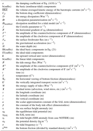
Fig. 2. (a) SSH

η

, (b) tidal height

η

η

η

−

η

in case TIDE, (e) data assimilation analysis

η

(Matsumoto et al., 2000) and (f)

η

in TIDEa1 at

the end of the 40-day experiments (20 Jun 2001 0:00 UTC). The same color shades are used in (b)-(f),

and red indicates ascend (positive) while blue descend (negative). The contour interval is 20 cm.

37

Fig. 2. (a) SSHη, (b) tidal heightηt, (c) height of the linear tidal componentηlt, (d) the differenceηt−ηltin case TIDE, (e) data assimilation

analysisη_ta(Matsumoto et al., 2000) and (f)ηtin TIDEa1 at the end of the 40-day experiments (20 June 2001 00:00 UTC). The same colors

are used in (b–f); red indicates ascend (positive), whereas blue indicates descend (negative). The contour interval is 20 cm.

who proposed an interpretation of horizontal viscosity as a way to parameterize the interaction between mesoscale ed-dies and internal waves. That is, the usage of different values means that mesoscale eddies interact differently with inter-nal waves that result from geostrophic adjustment than with internal tides. The experimental period was 10 days in M2, K1, M2v2 and M2v10.

In this paper, we analyzed the tidal heightηt defined by the SSH anomaly from NOTIDE,

ηt≡η−η(NOTIDE). (23)

It should be noted that this is in order to investigate pre-cisely the tidal field including secondary oscillations in the model. Actually, performing two simulations (one with and one without tides) is not required in order to obtain the tidal heights with some accuracy. Simulation output of the linear tidal component,ηlt, may serve as a basic data set of tides in an OGCM, since this component represents most of the tidal

variations as shown in Sect. 3.1. Alternatively, based on out-put ofη, the tidal heights can be estimated by the anomaly from the 25-hour running mean, or the deviation from the dy-namic heights after Arbic et al. (2010) (density data is needed in this case).

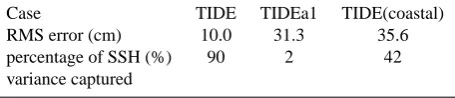
Table 3. The RMS error of the tidal height (cm) and the percentage

of SSH variance captured (%) in TIDE and TIDEa1. The values of “TIDE(coastal)” are calculated in the region shallower than 1000 m.

Case TIDE TIDEa1 TIDE(coastal)

RMS error (cm) 10.0 31.3 35.6

percentage of SSH (%) 90 2 42

variance captured

3 Results

3.1 Tidal height

The test experiments with our tidal scheme successfully re-produced many of the large-scale features known to be in the tidal field as well as basic field. Figure 2a shows the instan-taneous field of SSHηat the end of case TIDE. Tides with a basin scale are clearly seen, along with the geostrophic cir-culation on a large scale, (e.g. the meridional gradient of the Antarctic Circumpolar Current).

Figures 2b and 2c show the tidal heights,ηt, and the linear tidal component of SSH,ηlt, respectively, in TIDE. As noted in Sect. 2.2, the former represents the whole tidal motion, including nonlinear effects, while the latter is the primary barotropic response to the tidal forcing following Eqs. (11) and (12). Except for a few differences in coastal areas (10 cm at maximum), they are almost identical globally (Fig. 2d). This result supports our expectation that the linear tidal com-ponents,Ult andηlt, represent most of the tidal motions. In our new scheme, only the linear tidal equations adopt param-eterizations specified for tides; here, we suggest that this is enough to reproduce tides in a global model.

For comparison, Fig. 2e shows the tidal height of the re-analysis data set (Matsumoto et al., 2000),η_ta. The patterns of sea surface elevation inηt (or ηlt) of TIDE and ηat are very similar in the Indian, Pacific and Atlantic oceans, though there are some differences around the Antarctic continent. The amplitudes of these variables are also very similar. For example, the local maximum in the eastern equatorial Pacific region is approximately 87 cm in bothηt andηta. This result suggests that our new scheme worked as expected, and that the model reproduced a realistic time evolution of the tides.

By contrast,ηtin TIDEa1, which ignored the SAL term, is different fromηa_t (Fig. 2f). For example, the local maximum in the eastern Pacific was not located in the equatorial region, but adjacent to the west coast of North America, and the pat-tern of sea surface elevation around New Zealand deviated counterclockwise by approximately 60◦. The contrasting re-sults between TIDE and TIDEa1 indicate that realistic tides cannot be modeled in an OGCM if the original barotropic equation is used to calculate time evolution of tides. It is necessary to use parameterizations developed for tides. Even the scalar approximation for the SAL term, for example, im-proves simulations of the tides.

To investigate the causes of the differences between TIDE and TIDEa1 in detail, the amplitude of the tidal height varia-tion is evaluated by the root mean square ofηt,ηRMS,

ηRMS=



 

1 T1−T0

T1

Z

T0 η2_tdt



 

1/2

, (24)

whereT0 andT1 indicate 5 May 2001 and 20 June 2001,

i.e. the times after 10 and 40 days from the experiment start, respectively. Figure 3 showsηRMSin TIDE, TIDEa1 and the

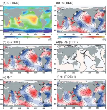
assimilation data set. ComparingηRMS(TIDE) and the

assim-ilation resultηa_RMS, the distributions and the local maxima are very similar except for some differences (e.g.,ηRMS is

slightly smaller in the Indian Ocean, and larger in the western equatorial Pacific region). Similarly,ηRMS(TIDEa1) is close

toηa_RMS, though its distribution seems somewhat distorted. The means by which the viscosity parameterization influ-ences the performance of the tidal amplitude is discussed in Sect. 3.2.

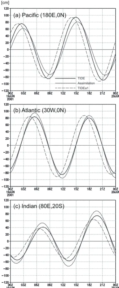
Next, the reproducibility of the tidal phase is examined. As representative results, Fig. 4 shows time series ofηt at three locations in the equatorial Pacific, the equatorial Atlantic and the central Indian Ocean. In contrast to the amplitudes, the re-producibility of the tidal phase differs substantially between TIDE and TIDEa1. Theηtphase is ahead by up to 1.5 h from ηa_t in TIDEa1 at all the locations (corresponding to 45◦for semi-diurnal tides). On the other hand,ηt is in phase withηat in TIDE, as the phase differences are found to be less than 0.5 h. As a result, the difference betweenηt andηtadecreases drastically in TIDE, in comparison with TIDEa1, nearly ev-erywhere. Thus, the problem of the tidal phase being too far ahead in TIDEa1 is corrected to some extent in TIDE. This is one important reason for the difference in the reproducibili-ties of the two cases shown in Fig. 2:

A possible mechanism of this correction is as follows. In-troduction of the SAL term modifies the gravitational accel-eration to αg virtually in TIDE, as indicated by Eq. (20). Since αis less than unity (0.88 in our settings), the phase velocity of shallow gravitational waves (√αg/H) becomes slower. This mechanism may contribute to reproducibility of the tidal phase.

The reproducibility of the tidal height is evaluated quanti-tatively here. For this purpose, a root-mean-squared error of ηt,ηRMSE, is calculated usingηat as a reference (Fig. 5),

ηRMSE≡



 

1 T1−T0

T1

Z

T0

(ηt−ηat)

2_dt



 

1/2

. (25)

In TIDE,ηRMSEis less than 20 cm – even in the open oceans

whereηRMSis large – and less than 10 cm in most other

1098 K. Sakamoto et al.: A practical scheme to introduce explicit tidal forcing into an OGCM

Discussion

P

ap

er

|

Discussion

P

ap

er

|

Discussion

P

ap

er

|

Discussion

P

ap

er

|

(a)

(TIDE)

(b)

(c)

(TIDEa1)

[cm]

Fig. 3. Root mean square of tidal height

η

(Eq. 24) in (a) TIDE, (b) assimilation analysis and (c)

TIDEa1. The contour interval is 5 cm.

38

Fig. 3. Root mean square of tidal height, ηRMS, (Eq. 24) in (a) TIDE, (b) assimilation analysis and (c) TIDEa1. The contour in-terval is 5 cm.

in most regions such that it reaches values comparable to ηRMSitself.

Following Arbic et al. (2004), who developed a highly-tuned two-layer tide prediction model without a data assim-ilation technique, the root-mean-squared error is averaged over the region ranging from 66◦_{S to 66}◦_{N with water depth}

exceeding 1000 m, which is indicated byA,

ηRMSE≡





1 A

Z Z

A

η_RMSE2 dxdy





1/2

, (26)

Discussion

P

ap

er

|

Discussion

P

ap

er

|

Discussion

P

ap

er

|

Discussion

P

ap

er

|

[cm]

TIDE

TIDEa1 Assimilation

(b) Atlantic (30W,0N) (a) Pacific (180E,0N)

(c) Indian (80E,20S)

Fig. 4. Time variation of tidal height

ηt

[cm] for 19-20 Jun 2001(day 40) in (a) the equatorial Pacific

(180

E, 0

N), (b) the equatorial Atlantic (30

W, 0

N), and (c) the central Indian Ocean (80

E, 20

S).

The thick, thin and dashed lines indicate TIDE, assimilation analysis and TIDEa1, respectively.

39

Fig. 4. Time variation of tidal heightηt [cm] for 19–20 June 2001

(day 40) in (a) the equatorial Pacific (180◦E, 0◦N), (b) the

equato-rial Atlantic (30◦W, 0◦N), and (c) the central Indian Ocean (80◦E,

20◦S). The thick, thin, and dashed lines indicate TIDE, assimilation

analysis, and TIDEa1, respectively.

where x and y are longitude and latitude, respectively. The RMSE in the SSH is as high as 31.3 cm in TIDEa1 and 10.0 cm in TIDE (Table 3). This is comparable to the RMSE found in previous studies (e.g. Jayne and St. Laurent, 2001; Arbic et al., 2004). In addition, Arbic et al. (2004) defined “a percentage of SSH variance captured” by 1−

K. Sakamoto et al.: A practical scheme to introduce explicit tidal forcing into an OGCM 1099

P

ap

er

|

Discussion

P

ap

er

|

Discussion

P

ap

er

|

Discussion

P

ap

er

|

[cm]

(a)

(TIDE)

(b)

(TIDEa1)

Fig. 5. Root mean square error of the tidal height

η

in (a) TIDE and (b) TIDEa1. The contour

interval is 5 cm.

40

Fig. 5. Root mean square error of the tidal height,ηRMSE, in (a) TIDE and (b) TIDEa1. The contour interval is 5 cm.

overA. The values are 90 % in TIDE, 2 % in TIDEa1, and 92 % in Arbic et al. (2004). The tide reproducibility is very low in TIDEa1, whereas in TIDE – due to taking into ac-count an approximation of the SAL term – it increases to the same level as a tuned tide model. Since a simple viscosity pa-rameterization was used in the experiment, the reproducibil-ity could increase further by adopting more sophisticated pa-rameterizations or tuning the settings more carefully. Though this task is beyond the scope of this paper, some case stud-ies discussed in Sect. 3.2 indicate that the tide reproducibility significantly depends on the viscosity settings.

To simulate circulations affected by tides, it is important to introduce tides realistically into an OGCM, even in coastal areas (e.g. Moon et al., 2010; Kurapov et al., 2010). However, the reproducibility of the tidal heights in coastal areas tended to decrease in our low-resolution model. The root-mean-squared errorηRMSEaveraged over the region shallower than

1000 m is found to be 35.6 cm, which is three times as large as the 10.0 cm ηRMSE in the open ocean, and the

percent-age of SSH variance captured is only 42 % (Table 3). This is likely because our low-resolution model cannot represent rel-atively small physical processes affecting coastal tides, such as excitement of internal tides over shelf slopes, waves break-ing on shelves, and the friction of complicated topographies (Xing and Davies, 1997; Osborne et al., 2011; Nagai and Hi-biya, 2012). Improvement of the coastal tides by the incorpo-ration of our scheme into a high-resolution OGCM is project to be completed in the future.

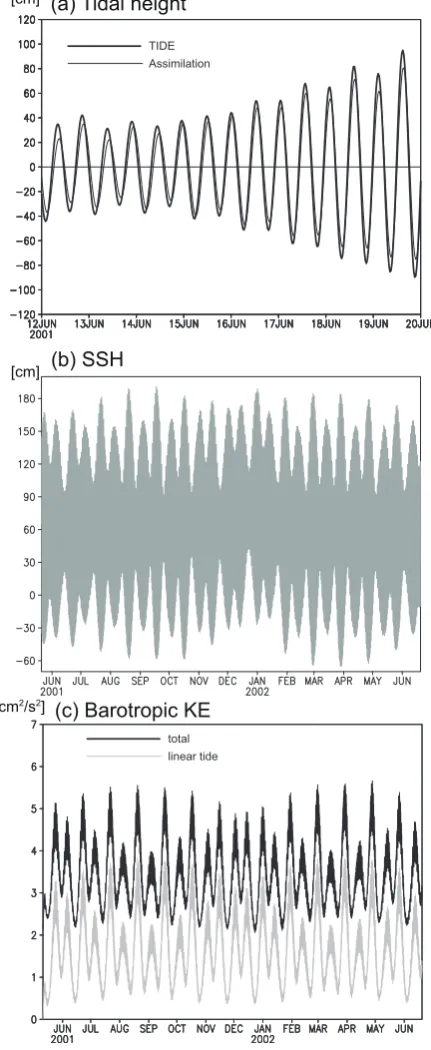
To verify that an OGCM with our tidal scheme runs stably, long time variations are analyzed here. First, the tidal heights ηt(TIDE) for 8 days are shown in Fig. 6a at the same location as Fig. 4a, together withηa_t. Amplitude modulation induced by neap and spring tides is found to be well reproduced in the model. Figure 6b shows the variation range ofη(TIDE) for one year at the same location. Quasi-stationary undulation of SSH is maintained for one year with fortnightly modulation. These results were obtained at the locations of Fig. 4b and

c, too (not shown). As systematic indices of the model sta-bility, the volume-averaged kinetic energy of the barotropic currents, BKE, and the counterpart of the linear tidal cur-rents, BKElt, are calculated by

BKE= 1

V

Z Z Z

V 1 2

U

H+η

2

dxdydz, (27)

BKElt= 1 V

Z Z Z

V 1 2

Ult H+η

2

dxdydz, (28)

where V indicates the whole region of the model (m3). Monotonic increase or decrease of energy is not found in the two time series of one year, though fortnightly variation ex-ists (Fig. 6c). It can be concluded that the model runs stably with our tidal scheme at least for one year.

3.2 Tidal motion

In this subsection, tidal motions reproduced by the new tidal scheme are validated using the results of cases M2 and K1. As shown in Fig. 2, most of the tidal height variation was represented by the linear tidal componentηlt in our global model. Similarly, barotropic currents with tidal frequencies were almost completely represented by the linear tidal com-ponentUlt, and thereforeUlt is used to compare with past tide studies. Hereafter, the 100-hour experimental results from 20:00 on day 6 (indicated byT0) to 24:00 on day 10

(T1) are used for analysis.

As a first step to validate the tidal currents in cases M2 and K1, Fig. 7 shows the mean speed distributions of the barotropic tidal currents,|ult|

t

, calculated by

|ult| t

= 1

T1−T0

T1

Z

T0

Ult H+η

1100 K. Sakamoto et al.: A practical scheme to introduce explicit tidal forcing into an OGCM

Discussion

P

ap

er

|

Discussion

P

ap

er

|

Discussion

P

ap

er

|

Discussion

P

ap

er

|

[cm] [cm]

(b) SSH (a) Tidal height

TIDE Assimilation

total linear tide

(c) Barotropic KE

[cm2_/s2_]

Fig. 6. (a) Same as Fig. 4 but for 12-20 Jun 2001 (day 32-40). The thick and thin lines indicate TIDE and

assimilation analysis, respectively. (b) The variation range of SSH at the site (180

◦

E, 0

◦

N) over one year

from 21 May 2001 to 20 Jun 2002 (day 10-405) in TIDE. (c) Same as (b) but for the volume-averaged

barotropic kinetic energy [cm

2

s

−

2

] of

U

(

BKE

, black) and

U

lt

(

BKE

lt

,gray).

41

Fig. 6. (a) Same as Fig. 4, but for 12–20 June 2001 (day 32–40). The

thick and thin lines indicate TIDE and assimilation analysis,

respec-tively. (b) The variation range of SSH at the site (180◦E, 0◦N) over

one year – from 21 May 2001 to 20 June 2002 (day 10–405) – in TIDE. (c) Same as (b) but for the volume-averaged barotropic

ki-netic energy [cm2s−2] ofU (BKE, black) andUlt (BKElt,gray).

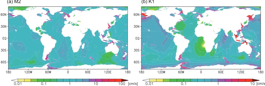
For both the M2 and K1 cases, the tidal currents are strong in coastal areas, especially near Great Britain, Ireland and east-ern Asia. In the M2 case,|ult|

t

is large over the Mid-Atlantic Ridge, and in the equatorial Pacific. In the K1 case,|ult|

t is large in the Indian Ocean and the North Pacific. These results agree well with Fig. 1 in Müller et al. (2010).

Next, we executed an energy analysis for the M2 tide. Gen-erally, the tide energy is supplied to interior ocean regions, and then transported to narrow coastal regions to be dissi-pated there. Egbert and Ray (2003) analyzed the pathways of the M2 tide energy based on an assimilation model. Follow-ing them, the tide energy flux,P, and the energy supply,W (i.e., the work which the tidal forcing does on the ocean), are estimated for the linear tidal component using

P = 1

T1−T0

T1

Z

T0

Ultηltdt (30)

W= 1

T1−T0

T1

Z

T0

Ult· ∇(βη0+ηSAL)dt. (31)

Assuming a steady energy state, the energy dissipation,D, can be estimated from the energy balance as

0=W− ∇ ·P−D. (32)

See Sect. 3.1 of Egbert and Ray (2001) for the derivation of these equations. Figure 8 verifies that the energy was sup-plied in interior regions, transported to coastal regions, and dissipated there. In addition, theP vector map agrees well with Egbert and Ray (2001). These results indicate that our model reproduced both the tidal heights and the tidal dynam-ics such as the tidal currents and the energy flux, which are important for effects on the basic fields. Figure 8b shows that the tidal energy dissipates over rough topographies such as the Izu-Ogasawara Ridge, the Hawaiian Ridge and the Central Atlantic Ridge, as well as in coastal regions. This likely reflects barotropic-to-baroclinic conversion resulting from excitement of internal tides over rough topographies (see Sect. 3.3).

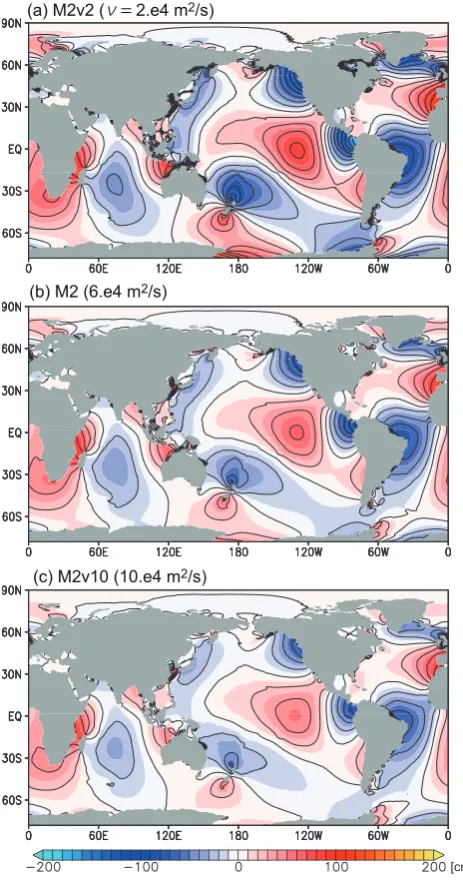
It has been shown that the precision of a tide model de-pends primarily on settings of viscosity and friction to dissi-pate tidal currents (Arbic et al., 2004). In our model experi-ments, tides also significantly depended on the viscosity set-tings, especially the horizontal viscosity,ν. Figure 9 shows ηt in the two additional cases where ν was decreased to 2×104m2s−1_{(case M2v2) and increased to 10×10}4_m2_s−1

K. Sakamoto et al.: A practical scheme to introduce explicit tidal forcing into an OGCM 1101

P

ap

er

|

Discussion

P

ap

er

|

Discussion

P

ap

er

|

Discussion

P

ap

er

|

(a) M2 (b) K1

[cm/s] [cm/s]

Fig. 7. Speed of the barotropic tidal currents

|

u

|

of (a) M2 tide and (b) K1 tide averaged over 100

hours from 20:00 on day 6 to 24:00 on day 10. The color shades are same as Fig. 1 of M¨uller et al.

(2010), and the units are cm s

.

42

Fig. 7. Speed of the barotropic tidal currents|ult|t of (a) M2 tide and (b) K1 tide averaged over 100 h from 20:00 on day 6 to 24:00 on day

10. The colors are the same as in Fig. 1 of Müller et al. (2010), and the units are cm s−1.

Discussion

P

ap

er

|

Discussion

P

ap

er

|

Discussion

P

ap

er

|

Discussion

P

ap

er

|

[m W/m2_]

[k W/m]

(a) W, P (b) -D

Fig. 8. (a) Tidal energy flux

P

(vector) and power on the ocean

W

[

10

W m

] (color shades) in case

M2. The unit length of the vectors is 200 k W m

the same as Fig. 1 of Egbert and Ray (2001). (b) Tidal

energy dissipation

−

D

in case M2. The 3000-m isobath is shown to illustrate the bottom topography.

43

Fig. 8. (a) Tidal energy fluxP(vector) and power on the oceanW(10−3Wm−2) (colored shading) in case M2. The unit length of the vectors

is 200 k Wm−1the same as Fig. 1 of Egbert and Ray (2001). (b) Tidal energy dissipation−Din case M2. The 3000 m isobath is shown to

illustrate the bottom topography.

between the water and the lateral boundary of bottom topog-raphy, rather than the viscosity of the interior currents or bot-tom friction (not shown). These results are consistent with Schwiderski (1980) and Arbic et al. (2004), who reported that interaction between tidal currents and bottom topogra-phy is one of the most important processes in dissipation of tides. As noted here, by using the new scheme, we could ad-just the tide viscosity and friction parameters, including in-teraction between tides and topography, without altering the original OGCM equations. This feature is essential to the re-alistic introduction of tides into an OGCM, as Arbic et al. (2010) pointed out.

3.3 Effects on basic fields

As noted in Sect. 2.2, our new tidal scheme is designed so that interaction processes between the basic fields and tides are represented in the original OGCM framework. Owing to this, the tidal effects on the basic fields would be reproduced naturally in the model, as long as the tidal currents are

gen-erated realistically by the scheme. Therefore, we expected that some changes would occur in the velocity and tracer fields of the test experiments, since the tidal currents were well reproduced. In order to validate impacts of our tidal scheme, changes in the basic fields are summarized briefly in this subsection, though the experimental period (40 days) and the model resolution (1◦×1/2◦) are not enough to rep-resent thorough modification of the basic fields in the real ocean.

suggest-1102 K. Sakamoto et al.: A practical scheme to introduce explicit tidal forcing into an OGCM

Discussion

P

ap

er

|

Discussion

P

ap

er

|

Discussion

P

ap

er

|

Discussion

P

ap

er

|

[cm]

(b) M2 (6.e4 m2_/s)

(c) M2v10 (10.e4 m2_/s)

(a) M2v2 ( 2.e4 m2_/s)

Fig. 9. Tidal height

η

at the end of the 40-day experiments (0:00 on 21 May 2001) in cases (a) M2v2

(

ν

= 2

×

10

m

s

), (b) M2 (

6

×

10

) and (c) M2v10(

10

×

10

). The contour interval is 20 cm.

44

Fig. 9. Tidal heightηt at the end of the 10-day experiments (00:00

on 21 May 2001) in cases (a) M2v2 (ν=2×104m2s−1), (b) M2

(6×104) and (c) M2v10 (10×104). The contour interval is 20 cm.

ing active excitement due to interaction between tides and topographies. This is consistent with the energy dissipation Din Fig. 8b.

Figure 10 shows thatw had a zonal band pattern with a meridional wavelength of approximately 200 km. This pat-tern is very similar to the result of Komori et al. (2008) (their Fig. 1), who simulated excitement of internal waves by wind using a model with a horizontal resolution of 1/4◦. However, Arbic et al. (2010) reported that internal tides have a ripple-like pattern spreading from bottom topographies, using an eddy-resolving model with a horizontal resolution of

approx-imately 1/10◦_{. Since reproducibility of internal tides depends}

strongly on model resolution (Niwa and Hibiya, 2011), this difference suggests that our model resolution of 1◦_×1/2◦

was not enough to represent internal tides.

To examine how the internal tides are excited in the model in more detail, potential densityσ0is analyzed around

Hawaii, where active excitement is expected from thew dis-tribution (Fig. 10). Figure 11a shows a time variation ofσ0

vertical distribution in TIDE and NOTIDE. No remarkable variation is found in NOTIDE (thin lines), while vertical un-dulation of the isopycnals with a period of half a day is clearly seen (thick lines). The amplitude reaches 50 m, which means that the model represented heaving of the isopycnals accompanied by internal tides. Figure 11b is a Hovmöller di-agram showing meridional and temporal change of potential density anomalyσ₀0 at the depth of 1000 m in TIDE, andσ₀0 is the anomaly from the time average as

σ₀0=σ0−

1 T1−T0

T1

Z

T0

σ0dt, (33)

whereT0andT1indicate 18 June 2001, 00:00 and 20 June,

00:00, respectively. In Fig. 11b, σ₀0 changed most dramat-ically over the rough topography around Hawaii (∼21◦N), showing oscillation with a period of half a day. Subsequently, the anomaly propagated northward and southward with de-cay (the arrows in the figure). Though the model meridional resolution of 0.5◦is clearly insufficient to represent the spa-tial structure of the internal tides, it can be concluded that excitement and propagation of the internal tides were repre-sented to some extent.

Fig. 12a shows another impact on the ocean, the sea sur-face temperature (SST) anomaly,1Tt,

K. Sakamoto et al.: A practical scheme to introduce explicit tidal forcing into an OGCM 1103

Discussion

P

ap

er

|

Discussion

P

ap

er

|

Discussion

P

ap

er

|

Discussion

P

ap

er

|

Fig. 10. Vertical velocity

w

[cm s

] at 1900 m depth in the North Pacific in (a) TIDE and (b) NOTIDE.

The instantaneous distributions at the end of the 40-day experiment are shown.

45

Fig. 10. Vertical velocityw(cm s−1) at 1900 m depth in the North Pacific in (a) TIDE and (b) NOTIDE. The instantaneous distributions at the end of the 40-day experiment are shown.

Discussion

P

ap

er

|

Discussion

P

ap

er

|

Discussion

P

ap

er

|

Discussion

P

ap

er

|

Fig. 11. (a) Vertical distribution of potential density

σ

[kg m

] from bottom to the 1000-m depth at

(55

W, 20

N) for 18-20 Jun 2001 (day 39-40) of TIDE (thick lines and color shade) and NOTIDE (thin

lines). (b) Hovm¨oller diagram of potential density anomaly

σ

at 55

W, 1000-m depth in TIDE. The

meridional range is 16-24

N, and the time period is the same as (a). The arrows indicate propagation of

internal tides.

46

Fig. 11. (a) Vertical distribution of potential densityσ0(kg m−3) from bottom to the 1000 m depth at (55◦W, 20◦N) for 18–20 June 2001

(day 39–40) of TIDE (thick lines and colored shading) and NOTIDE (thin lines). (b) Hovmöller diagram of potential density anomalyσ₀0 at

55◦W, 1000-m depth in TIDE. The meridional range is 16–24◦N, and the time period is the same as (a). The arrows indicate propagation

of internal tides.

surface cooling. Both temperature and salinity were almost uniform from the surface to the depth of 80m. Another rea-son may be that representation of the tidal mixing was not adequate due to the low resolution of our model. Low reso-lution is also likely responsible for the fact that large vertical diffusivities were only intermittently predicted in the North-ern Hemisphere.

The SST decrease with the inclusion of tides was espe-cially large in shallow coastal regions; e.g., more than 1◦C around the islands of Great Britain and Ireland. Since this de-crease was accompanied with weakening of stratification, the reason is likely that strong tidal currents (Fig. 7) induced ver-tical mixing through shear instability in the bottom layer, as reported by observational and numerical studies about tidal fronts (Simpson and Hunter, 1974; Müller et al., 2010). The SST anomaly was also large in some polar coastal seas, such

as the Greenland Sea and the Ross Sea. This is consistent with the findings of previous studies, which showed signifi-cant tidal impacts on dense water formation processes there (Pereira et al., 2002; Robertson, 2001a, b).

1104 K. Sakamoto et al.: A practical scheme to introduce explicit tidal forcing into an OGCM

Discussion

P

ap

er

|

Discussion

P

ap

er

|

Discussion

P

ap

er

|

Discussion

P

ap

er

|

Fig. 12. (a) SST difference between TIDE and NOTIDE∆Tt[C◦]. (b) Vertical profiles of temperature

Ttat the site (50◦W, 50◦N) (marked in (a)) in TIDE (thick line) and NOTIDE (thin). The vertical range from surface to 65 m depth is shown. Both of (a) and (b) use 25-hour averages of the end of the 40-day experiments.

47

Fig. 12. (a) SST difference between TIDE and NOTIDE1Tt(C◦). (b) Vertical profiles of temperatureTtat the site (50◦W, 50◦N) (marked in (a)) in TIDE (thick line) and NOTIDE (thin). The vertical range from surface to 65 m depth is shown. Both (a) and (b) use 25-hour averages of the end of the 40-day experiments.

TIDE and NOTIDE reached approximately 10 % of the total velocity in two months. However, it did not expand further after that.)

Though plausible impacts on the OGCM were obtained by our scheme as for impacts of tidal currents, it should be noted that our experiment is the initial investigation of the scheme. In particular, the horizontal resolution of the model is too low to represent internal tides or tidal mixing processes (Mat-sumoto et al., 2000). With implementation of this scheme in a higher resolution OGCM, evidence of barotropic to baro-clinic energy conversion can be provided directly via vertical velocity and potential density, and the conversion rate and coastal effects (Simmons et al., 2004) can be investigated in more detail. A thorough investigation about the process for tidal currents to intensify vertical mixing through velocity shear and turbulence will also be possible. We plan to exe-cute a long-term experiment in order to examine the tidal im-pacts, including dependencies on model resolution or mixing parameterizations, in more detail.

4 Conclusions

A new practical scheme is proposed to introduce tides ex-plicitly into ocean general circulation models (OGCMs). In this scheme, barotropic linear response to the tidal forcing is calculated by the time differential equations modified for ocean tides, instead of the original barotropic equations of the OGCM. This allows for the usage of various parameteri-zations specified for tides, such as the self-attraction/loading (SAL) effect and energy dissipation due to internal tides, without unintentional violation of the original dynamical bal-ances in an OGCM. Owing to this feature, the knowledge of barotropic tide modeling can be exploited to improve repro-ducibility of tides in an OGCM. In other words, this scheme

drives an OGCM by the barotropic tidal currents which are predicted progressively by a tuned tide model, in lieu of us-ing the equilibrium tidal potential. The numerical cost of the scheme is comparable to the barotropic calculation of the original OGCM.

We incorporated this scheme into Meteorological Re-search Institute Community Ocean Model (MRI.COM) and executed test experiments with a low-resolution global model (1◦×1/2◦). The results showed that the model could simu-late tides realistically without affecting the basic fields un-intentionally, and that the model runs stably for at least one year. The root-mean-squared error of the tidal heights was only 10.0 cm in the reference of a data-assimilation result, suggesting that the tide reproducibility is comparable to that of tide models tuned elaborately. By contrast, when the SAL term was ignored, the reproducibility decreased significantly, as the error rose to 31.3 cm. This suggests that the SAL scalar parameterization must be utilized in order to introduce tides into an OGCM realistically. Although this conclusion has been drawn by Arbic et al. (2010), our methodology is dif-ferent from theirs.

since the nonlinearity becomes relatively strong there. By investigating how the tide reproducibility in an OGCM de-pends on the selection of the two schemes, validation of their approximations can be tested under realistic situations. We believe that this problem is worthy of study in order to fur-ther refine the tide schemes.

It should be noted that our model settings were rather crude. Recently, sophisticated parameterizations for tidal en-ergy dissipation have been proposed by studies about the interaction between tides and topography (e.g. Jayne and St. Laurent, 2001). The tide reproducibility may improve fur-ther by adopting such parameterizations, making use of the feature that lets the tide settings be decided independently of which OGCM is used. Actually, our case studies showed that the reproducibility depends sharply on the configuration of the viscosity related to topography, suggesting a possi-ble contribution of such parameterizations. Model sensitiv-ity to bottom drag parameterizations should be investigated with this scheme, too. Though we used the Weatherly et al. (1980) and Schwiderski (1980) parameterizations for the ba-sic and linear tidal components, respectively, they have not been tested in the situation where both of the tidal currents and the geostrophic circulations exist. Thus, implementing the appropriate tidal parameterizations in an OGCM in the framework of our new scheme remains to be carried out. In order to do this, it is also necessary to systematically evalu-ate errors in the phase and the amplitude of each tidal con-stituent, which is not analyzed in this paper. We plan to do this using our model, MRI.COM.

In spite of the crude settings, our model generally repro-duced similar amplitudes of the M2 and K1 tidal currents and the tidal energy conversions when compared with previ-ous tidal modeling studies. In addition, excitement of inter-nal tides and enhancement of vertical mixing were found in the model, though the experimental period was as short as 40 days. We did this by generating the realistic tidal currents in the model through an explicit tidal scheme, in contrast to the indirect parameterizations of tidal mixing used by many traditional OGCMs, such as additional increase of the back-ground vertical diffusivity. Usage of our scheme is expected to improve representation of various physical processes, such as water exchange between coastal and open oceans, and even chemical and biological processes (e.g. Sect. 8.6 of Simpson and Sharples, 2012). Explicit introduction of tides into an OGCM is a significant step towards upgrading ocean modeling. We plan to investigate the impacts in more detail using a model with a finer resolution.

Appendix A

Modification of tides

Tides affect the basic field as shown in Sect. 3.3, and in turn, the basic field modifies the tides. For example, when density

stratification exists, kinetic energy conversion occurs from barotropic tides to internal tides. In the new tide scheme, the linear tidal component represents the primary barotropic response to the equilibrium tide potential, and does not in-clude such modification. This appendix explains how such modification is represented in the framework of the new tide scheme.

To treat the question clearly and analytically, we consider a simple situation as follows. The ocean state is thoroughly horizontally uniform, including the tidal forcing, and dissi-pation and bottom friction are ignored. Under these assump-tions, the momentum equation of the linear tidal component, Eq. (12), is simplified as

∂Ult

∂t −f Vlt=gHβ ∂η0

∂x (A1)

∂Vlt

∂t +f Ult=gHβ ∂η0

∂y , (A2)

whereUandV indicate the components of the velocity vec-torU=(U, V ). Now, introducing complex number expres-sions

Ult=Ult+iVlt (A3)

F=∂η0

∂x +i ∂η0

∂y , (A4)

Eqs. (A1) and (A2) combine to become ∂Ult

∂t +ifUlt=gHβF. (A5)

We assume a horizontal vector varying trigonometrically with frequencyσfor the tidal forcingF, and as a result, both

UltandF can be deformed to a sum of the two rotary com-ponents in general as follows (Davies, 1985; Sakamoto and Akitomo, 2006):

U_lt=R_lt+eiσ t+R_lt−e−iσ t (A6)

F=F+eiσ t+F−e−iσ t

, (A7)

whereR_lt+andF+ are the amplitudes of the counterclock-wise components, whileR_lt−andF−are those of the clock-wise components. Substituting Eqs. (A6) and (A7) into Eq. (A5), we obtain the solution ofUltforF,

R_lt+= gHβ

i(σ+f )F

+

(A8) R_lt−= gHβ

i(−σ+f )F

−

. (A9)

1106 K. Sakamoto et al.: A practical scheme to introduce explicit tidal forcing into an OGCM

the assumptions of Eqs. (A1) and (A2), the barotropic mo-mentum equation of the basic component Eq.(13), i.e., the original equation of OGCM , is simplified to

∂Ub

∂t +ifUb=X, (A10)

whereUbis a complex number,

Ub=Ub+iVb, (A11)

andX represents the secondary interactions. Here, we as-sume a linear damping forX. Modeling the barotropic tides as dissipated by excitation of the internal tides due to a com-bination of tidal currents and stratification,

X= −aUlt. (A12)

The constanta is a damping coefficient with units of s−1. Now we deformUbto a sum of the two rotary components in the same manner as in Eq. (A6):

Ub=R+_beiσ t+R−_be−iσ t. (A13) Substituting Eqs. (A12) and (A13) into Eq. (A10), we obtain a modification of the tidal currents induced by the secondary interaction,X:

R_b+= −a

i(σ+f )R

+

lt (A14)

R_b−= −a

i(−σ+f )R

−

lt. (A15)

The actual tidal currents are a sum of the linear tidal com-ponent, Ult, and the modification due to the secondary in-teractions. Since th