Ocean Sci., 4, 31–47, 2008 www.ocean-sci.net/4/31/2008/
© Author(s) 2008. This work is licensed under a Creative Commons License.
Ocean Science
Operational ocean forecasting in the Eastern Mediterranean:
implementation and evaluation
G. Zodiatis1, R. Lardner1, D. R. Hayes1, G. Georgiou1, S. Sofianos2, N. Skliris2, and A. Lascaratos2
1Oceanography Centre, University of Cyprus, P.O. Box 20537, 1678 Nicosia, Cyprus
2Applied Physics Dept., Ocean Physics Modelling Group, University of Athens, Athen, Greece
Received: 28 March 2006 – Published in Ocean Sci. Discuss.: 8 June 2006
Revised: 6 September 2006 – Accepted: 11 December 2007 – Published: 4 February 2008
Abstract. The Cyprus Coastal Ocean Forecasting and Ob-serving System (CYCOFOS) has been producing operational flow forecasts of the northeastern Levantine Basin since 2002 and has been substantially improved in 2005. CYCOFOS uses the POM flow model, and recently, within the frame of the MFSTEP project, the flow model was upgraded to use the hourly SKIRON atmospheric forcing, and its resolution was increased from 2.5 km to 1.8 km. The CYCOFOS model is now nested in the ALERMO regional model from the Uni-versity of Athens, which is nested within the MFS basin model. The Variational Initialization and FOrcing Platform (VIFOP) has been implemented to reduce the numerical tran-sient processes following initialization. Moreover, a five-day forecast is repeated every day, providing more detailed and more accurate information. Forecast results are posted on the web page http://www.oceanography.ucy.ac.cy/cycofos. The new, daily, high-resolution forecasts agree well with the ALERMO regional model. The agreement is better and re-sults more reasonable when VIFOP is used. Active and slave experiments suggest that a four-week active period produces realistic results with more small-scale features. For runs in September 2004, biases with remote sensing sea surface tem-perature are less than 0.6◦C with similar expressions of the flow field present in both. Remotely-observed coastal up-welling south of Cyprus and advection of cool water from the Rhodes Gyre to the southern shores of Cyprus are also modeled. In situ observed hydrographic data from south of Cyprus are similar to the corresponding forecast fields. Both indicate the relatively fresh subsurface Atlantic Wa-ter and a near-surface anticyclone south of Cyprus for Au-gust/September of 2004 and September 2005. Plans for fur-ther model improvement include assimilation of observed XBT temperature profiles, CTD profiles from drifters and gliders, and CT data from the CYCOFOS ocean observatory.
Correspondence to: D. R. Hayes
1 Introduction
Forecasting seawater movements and properties is of impor-tance in understanding the effects of human activities on the marine environment as well as the effect of marine conditions on human operations in the sea. Flow modelling is consid-ered a useful operational tool for decision-making in case of marine accidents. Some examples where operational fore-casting is vital include search and rescue, oil spill fate mod-elling, and dispersion of pollutants. The practical real-time benefits of operational oceanography also bring improved understanding of environmental conditions and change at many levels. These operational activities imply a close at-tention to marine conditions on a daily basis over a period of years and from basin scales down to coastal scales.
30’ 32oE 30’ 33oE 30’ 34oE 30’ 35oE 30’ 36oE 30’
34oN
30’
35oN
30’
36oN
30’
500 1000 1500 2000 2500 Depth (m)
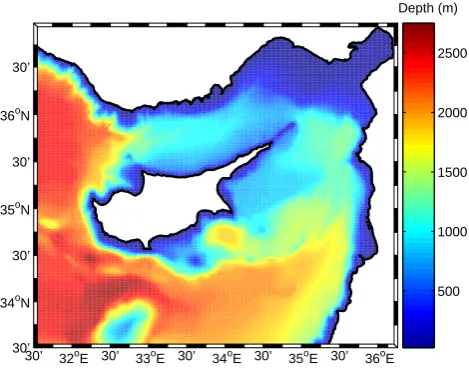
Fig. 1. Bathymetry and domain of CYCOM.
The known features of the general circulation near Cyprus as well as the climatological output for CYCOM are dis-cussed by Zodiatis et al. (2003). In summary, Cyprus has no significant river discharge, very narrow coastal areas with steep topographic gradients for shelf breaks and a shoreline exposed to the open sea. The coastal/shelf areas of the Levan-tine Basin are dominated by the mesoscale flow phenomena of the neighboring deep regions, such as the jet of Atlantic Water that meanders south of Cyprus, the Asia Minor Cur-rent, the Rhodes Gyre, and various eddies that can persist south of Cyprus for months. Storm surges are not important because of only moderate storm intensity, small tidal range (less than 0.3 m), and generally steep coastlines. Only the near-surface layers are affected by persistent westerly winds, which result in an upwelling feature on the southern or south-western coast of Cyprus.
2 Methods and model descriptions
Both CYCOM and ALERMO use numerical schemes that are modified versions of POM (the Princeton Ocean Model). The POM model has been widely used both within the frame-work of the MFS and elsewhere to simulate the flows in both regional and subregional sea areas of the Mediterranean Sea. POM has been extensively described in the literature (Blumberg and Mellor, 1987; Lascaratos and Nittis, 1998; Zavatarelli and Mellor, 1995). The POM model is a primitive equation, 3-D ocean circulation model based on the full non-linear equations of momentum and mass conservation and their depth-averaged forms. The model comprises a bottom-following sigma coordinate system, a free surface, and split mode time steps. At each time-step, the surface elevation and vertically integrated mass transports (that is, the barotropic mode) are computed from the depth-averaged equations by an explicit leapfrog scheme. The vertical structure of the current (baroclinic mode) is obtained from the horizontal
momentum equations with a longer time step (Lardner and Cekirge, 1998). Advancing the baroclinic mode is compu-tationally much more demanding and the use of a longer time step for it makes the overall computational scheme quite efficient. All sub-grid-scale phenomena are considered as mixing processes by introducing separate horizontal and ver-tical mixing terms. The horizontal viscosity and diffusion terms are evaluated using the Smagorinsky (1963) horizontal diffusion formulation while the vertical mixing coefficients for momentum and tracers are computed according to the Mellor-Yamada 2.5 turbulence closure scheme (Mellor and Yamada, 1982). Heat and salinity transport sub-models are included. Potential temperature, salinity, velocity and sur-face elevation, are the prognostic variables of the model. 2.1 Cyprus Coastal Model (CYCOM)
The domain of CYCOM (Fig. 1) is bounded by coastline on the north and east (maximum latitude of 36◦550N and maximum longitude of 36◦130E). The open boundary to the south is the 33◦300N latitude line, and the open boundary to the west is the 31◦300E meridian. Horizontal Cartesian co-ordinates are in the Mercator projection with an Arakawa C-grid, and the resolution is uniform at one minute (ap-proximately 1.8 km) for a total of 284×206 horizontal grid points. The grid-spacing is sufficiently small to resolve steep bathymetry in the region as well as features with internal Rossby radius length scales (10–15 km). In the vertical, a non-uniform grid of 25 sigma layers was used with expo-nentially decreasing spacing near the surface and sea bed to provide finer resolution of the surface and bed layers. The bottom topography is based on the 10×10 U.S. Navy Dig-ital Bathymetric Database. The minimum depth is 20 m. The equations used in CYCOM are described in Zodiatis et al. (2003).
G. Zodiatis et al.: Operational ocean forecasting: Eastern Mediterranean 33
24.5 25 25.5 26 26.5 27 27.5 28 28.5
30’ 32oE 30’ 33oE 30’ 34oE 30’ 35oE 30’ 36oE
30’
34oN
30’
35oN
30’
36oN
30’
(deg C)
24.5 25 25.5 26 26.5 27 27.5 28 28.5
30’ 32oE 30’ 33oE 30’ 34oE 30’ 35oE 30’ 36oE
30’
34oN
30’
35oN
30’
36oN
30’
(deg C)
−1 −0.8 −0.6 −0.4 −0.2 0 0.2 0.4 0.6 0.8 1
30’ 32oE 30’ 33oE 30’ 34oE 30’ 35oE 30’ 36oE
30’
34oN
30’
35oN
30’
36oN
30’
(deg C) −1
−0.8 −0.6 −0.4 −0.2 0 0.2 0.4 0.6 0.8 1
30’ 32oE 30’ 33oE 30’ 34oE 30’ 35oE 30’ 36oE
30’
34oN
30’
35oN
30’
36oN
30’
(deg C)
(a)
(c)
(b)
(d)
Fig. 2. Sea surface temperature for operational mode forecasts from (a) ALERMO (b) CYCOM, using the VIFOP method of initialization. (c) The temperature difference field of (a) and (b). (d). The same as (c) but using the CYCOM forecast that did not use VIFOP. The output
fields are 24-h averages on 2 October 2005, which was the fourth day of the forecast.
Surface and bottom boundary conditions are applied as described in Zodiatis et al. (2003). Surface boundary forc-ing is provided by the SKIRON 5-day forecast (Kallos et al., 1997). The high-resolution (0.1◦) and high-frequency
(hourly) forecast is available daily and starts at midnight. It provides 10-m wind speed, 2-m air temperature and relative humidity, the precipitation rate, the shortwave radiative gain by the ocean and the infrared atmospheric radiation reach-ing the sea surface. These daily atmospheric forecasts are used for each new ocean forecast using the bulk flux formula-tion. Downward shortwave and longwave radiation are used directly from SKIRON, while heat loss terms are calculated from SKIRON-provided parameters. Sensible and latent heat are calculated from Budyko (1963), longwave loss is calcu-lated from Bignami (1995). Evaporation is also calcucalcu-lated from Budyko (1963) and combined with SKIRON-provided precipitation for surface salinity flux. Surface momentum fluxes are calculated using the computed drag coefficient of Hellerman and Rosenstein (1983). There is no relaxation of surface fields.
The daily average fields required by the MFSTEP project for all partners are posted on the web site: http://www.oceanography.ucy.ac.cy/cycofos. Five subre-gions can be viewed online and forecast data can be down-loaded for user-visualization using the Visual Interface of Oceanographic Data, VIOD, or for use in the oil spill model,
0 5 10 15 20 25 30
0 0.05 0.1 0.15 0.2 0.25 0.3 0.35
Day of January 2005
standard deviation of DT (deg C)
T0 (slave − slave)
T0 (active − slave) T30 (slave − slave)
T30 (active − slave)
Fig. 3. Root-mean-square differences of temperature between
var-ious runs throughout the January 2005 experiment. Solid lines are for surface temperature, dotted are for 30 m. Cyan line is for ALERMO slave minus CYCOM slave. Green line is for ALERMO active minus CYCOM active.
30’ 32o
E 30’ 33oE 30’ 34oE 30’ 35oE 30’ 36oE
30’
34oN
30’
35oN
30’
36oN
30’
(deg C)
ALERMO slave 00:00 GMT January 12, 2005
16 16.5 17 17.5 18 18.5 19
30’ 32o
E 30’ 33oE 30’ 34oE 30’ 35oE 30’ 36oE
30’
34oN
30’
35oN
30’
36oN
30’
(deg C)
CYCOM slave 00:00 GMT January 12, 2005
16.5 17 17.5 18 18.5 19
30’ 32oE 30’ 33oE 30’ 34oE 30’ 35oE 30’ 36oE
30’
34oN
30’
35oN
30’
36oN
30’
(deg C)
ALERMO active 00:00 GMT January 12, 2005
16.5 17 17.5 18 18.5 19
30’ 32oE 30’ 33oE 30’ 34oE 30’ 35oE 30’ 36oE
30’
34oN
30’
35oN
30’
36oN
30’
(deg C)
CYCOM active 00:00 GMT January 12, 2005
16.5 17 17.5 18 18.5 19
30’ 32o
E 30’ 33oE 30’ 34oE 30’ 35oE 30’ 36oE
30’
34oN
30’
35oN
30’
36oN
30’
(deg C)
NOAA−16 00:31 GMT January 12, 2005
16.5 17 17.5 18 18.5 19
(a)
(c)
(b)
(d)
(e) (f)
−0.5 −0.4 −0.3 −0.2 −0.1 0 0.1 0.2 0.3 0.4 0.5
30’ 32oE 30’ 33oE 30’ 34oE 30’ 35oE 30’ 36oE
30’
34oN
30’
35oN
30’
36oN
30’
(deg C)
Fig. 4. Sea surface temperature comparison for day 12 of active-slave experiment. (a) ALERMO slave. (b) CYCOM slave. (c) ALERMO
active. (d) CYCOM active. (e) Difference between ALERMO slave and CYCOM slave. (f) Remotely-sensed image for the same day. ALERMO figures are 24-h averages, while CYCOM images are 6-h averages.
The ALERMO model covers the geographical area 20◦E– 36.4◦E, 30.7◦N–41.2◦N and has one open boundary located at 20◦E as shown in Fig. 1. The computational grid has a horizontal resolution of 1/30◦×1/30◦(493×316 grid points), 25 sigma levels, and a minimum depth of 25 m. The one-way nesting with the global Mediterranean OGCM is applied along the western boundary of ALERMO and is described in Korres and Lascaratos (2003).
2.2 Operational mode
G. Zodiatis et al.: Operational ocean forecasting: Eastern Mediterranean 35
14
G. Zodiatis et al.: Operational ocean forecasting: Eastern Mediterranean
14 15 16 17 18 19
14 14
14
14.5 15 14.5 14.5
15
15 15.5
15.5
15.5
16 16 16
16.5
16.5 16.5
17 17 17
17.5
17.5 17.5
18 18 18
18.5 18.5 18.5
Ocean Data View
100 200 300
0
100
200
300
400
500
600
Ocean Data V
iew
14 15 16 17 18 19
0
100
200
300
400
500
600
30°E 31°E 32°E 33°E 34°E 35°E 32°N
33°N 34°N 35°N
O
cean
Dat
a
View
Temperature (deg C)
Depth (m)
Distance (km)
Depth (m)
Temperature (deg C)
Fig. 5.
Expendable bathythermograph section from 13–14 January
2005.
Fig. 5. Expendable bathythermograph section from 13–14 January 2005.
project for end users. Instantaneous fields could also have been used without difficulty.
A second run on Thursdays was initialized with the instan-taneous fields of the first run and forced with the Thursday SKIRON forecast. Forecasts run days other than Thursday were also initialized with an instantaneous field from a pre-vious CYCOM forecast, and applied the newly available at-mospheric forecast. At the time of this study, ALERMO was running weekly, so some of the daily CYCOM forecasts used MFS basin model lateral boundary conditions. In this way, it was possible to compute 4.5-day forecasts every day. Cur-rently, ALERMO is running daily, and the CYCOM daily run is using the current day’s SKIRON meteorological fore-cast and lateral boundary conditions from ALERMO.
3 Results
3.1 Model-model comparisons
3.1.1 Downscaling from regional to coastal models When initializing CYCOM, it is important to maintain agree-ment with the basin model (and therefore ALERMO), since it has assimilation of observed data. A forecast produced on 28 September 2005 is now examined in order to
com-pare the results of two methods of downscaling: bilinear interpolation and Variational Initialization (VI). During the period of 28 September to 17 October 2005, both methods were used in two parallel forecasting systems for compari-son, after which the bilinear method was stopped. Average CYCOM fields of sea surface temperature centered at noon of the fourth day of the forecast, 2 October 2005 are com-pared with the ALERMO forecast on the same day (fifth day for that forecast) (Fig. 2). Comparison is better when the bilinear interpolation method is replaced by the VIFOP method of downscaling. The use of VIFOP reduces errors when an interpolated velocity interacts with high-resolution coastal features not present in the lower resolution model. Most importantly, using VIFOP improves flow direction and strength in many cases. Flow into the coast is less com-mon. Errors in surface temperature are also seen when us-ing bilinear interpolation. The surface temperature field pro-duced by ALERMO (Fig. 2a) and CYCOM using the VI-FOP method (Fig. 2b) differ in small areas near the coast (Fig. 2c). In these regions, the models differ by a few tenths of a degree Celsius up to 1◦C for a very small number of grid points. Over the whole domain, the mean difference is
24.5 25 25.5 26 26.5 27 27.5 28 28.5 29 29.5
30’ 32oE 30’ 33oE 30’ 34oE 30’ 35oE 30’ 36oE 30’
34oN 30’ 35oN 30’ 36oN 30’ (deg C) 24.5 25 25.5 26 26.5 27 27.5 28 28.5 29 29.5
30’ 32oE 30’ 33oE 30’ 34oE 30’ 35oE 30’ 36oE 30’
34oN 30’ 35oN 30’ 36oN 30’
(deg C)
30’ 32oE 30’ 33oE 30’ 34oE 30’ 35oE 30’ 36oE 30’
34oN 30’ 35oN 30’ 36oN 30’ (deg C) 25 25.5 26 26.5 27 27.5 28 28.5 29
30’ 32oE 30’ 33oE 30’ 34oE 30’ 35oE 30’ 36oE 30’
34oN 30’ 35oN 30’ 36oN 30’ (deg C) 25 25.5 26 26.5 27 27.5 28 28.5 29
30’ 32oE 30’ 33oE 30’ 34oE 30’ 35oE 30’ 36oE 30’
34oN 30’ 35oN 30’ 36oN 30’ (deg C) 25 25.5 26 26.5 27 27.5 28 28.5 29
30’ 32oE 30’ 33oE 30’ 34oE 30’ 35oE 30’ 36oE 30’
34oN 30’ 35oN 30’ 36oN 30’ (deg C) 25 25.5 26 26.5 27 27.5 28 28.5 29
30’ 32oE 30’ 33oE 30’ 34oE 30’ 35oE 30’ 36oE 30’
34oN 30’ 35oN 30’ 36oN 30’ (deg C) 25 25.5 26 26.5 27 27.5 28 28.5 29
30’ 32oE 30’ 33oE 30’ 34oE 30’ 35oE 30’ 36oE 30’
34oN 30’ 35oN 30’ 36oN 30’ (deg C) 25 25.5 26 26.5 27 27.5 28 28.5 29
30’ 32oE 30’ 33oE 30’ 34oE 30’ 35oE 30’ 36oE 30’
34oN 30’ 35oN 30’ 36oN 30’ (deg C) 25 25.5 26 26.5 27 27.5 28 28.5 29
30’ 32oE 30’ 33oE 30’ 34oE 30’ 35oE 30’ 36oE 30’
34oN 30’ 35oN 30’ 36oN 30’ (deg C) 25 25.5 26 26.5 27 27.5 28 28.5 29
30’ 32oE 30’ 33oE 30’ 34oE 30’ 35oE 30’ 36oE 30’
34oN 30’ 35oN 30’ 36oN 30’ (deg C) 25 25.5 26 26.5 27 27.5 28 28.5 29
30’ 32oE 30’ 33oE 30’ 34oE 30’ 35oE 30’ 36oE 30’
34oN 30’ 35oN 30’ 36oN 30’ (deg C) 25 25.5 26 26.5 27 27.5 28 28.5 29
30’ 32oE 30’ 33oE 30’ 34oE 30’ 35oE 30’ 36oE 30’
34oN 30’ 35oN 30’ 36oN 30’ (deg C) 25 25.5 26 26.5 27 27.5 28 28.5 29
30’ 32oE 30’ 33oE 30’ 34oE 30’ 35oE 30’ 36oE 30’
34oN 30’ 35oN 30’ 36oN 30’ (deg C) 25 25.5 26 26.5 27 27.5 28 28.5 29
30’ 32oE 30’ 33oE 30’ 34oE 30’ 35oE 30’ 36oE 30’
34oN 30’ 35oN 30’ 36oN 30’ (deg C) 25 25.5 26 26.5 27 27.5 28 28.5 29
Fig. 6. SST comparison between remote-sensing, CYCOM active, ALERMO slave (from left to right). Dates are from top to bottom: 3, 8,
G. Zodiatis et al.: Operational ocean forecasting: Eastern Mediterranean 37
15 17.5 20 22.5 25 27.5
16
16
18 18
20 22 20 22
24 26 24 26
15 28
17
17
O
cean
Dat
a Vi
ew
34.5°N 34°N 33.5°N 33°N 32.5°N
50
100
150
200
250 38.5 38.6 38.7 38.8 38.9 39 39.1 39.2 39.3
38.8
38.8
38.8 38.8
38.9
38.9
38.9 38.9
39 39
39
39 39
39.2 39.2
O
cean
Dat
a
Vi
ew
34.5°N 34°N 33.5°N 33°N 32.5°N
50
100
150
200
250
14 14.5 14
14.5
15 15.5 16 1515.5
13 .75
13.75
O
cean
Dat
a
Vi
ew
34.5°N 34°N 33.5°N 33°N 32.5°N
500
1000
1500
2000
38.8 38.8
38.9 38.9
39 39
38.75 38.75 38.8538.95 38.85
38.95
O
cean
Dat
a
Vi
ew
34.5°N 34°N 33.5°N 33°N 32.5°N
500
1000
1500
2000
32°E 33°E 34°E
32°N 33°N 34°N 35°N
O
c
ean
Dat
a V
iew
S N
N Salinity (psu) Temperature (deg C)
Depth (m)
-15 -10 -5 0 5 10 15 20
-15
-15
-12 .5
-1 2.
5
-10
-1 0
-7 .5
-7 .5 -7.5
-5
-5
-5
-5
-5
-2 .5
-2.5
-2.
5
-2.5
-2 .5
0
0
0
0
2.5
2.5
2
.5
2.5
5 5
7.5 10
O
cean Dat
a
Vi
ew
34.5°N 34°N 33.5°N 33°N 32.5°N
0
100
200
300
400
500
Ocean Data View
S
N Geostrophic velocity rel. to 700 m (cm/s)
Depth (m)
Fig. 7. (a) and (b) Hydrographic section along 33◦E collected during CYBO-18 (16–25 August 2004). (c) Zonal geostrophic velocity
relative to 700 m.
to the coast of Cyprus (Fig. 2d). In this case, the mean tem-perature difference is−0.0357◦C and standard deviation is
0.238◦C. Assuming a normal distribution and using the num-ber of ALERMO ocean points in the Cyprus region (12 569), the difference field is not distinguishable from zero at the 95% confidence level when using VIFOP. When using bilin-ear interpolation, the bias is significant.
3.1.2 Slave-active comparisons
15 17.5 20 22.5 25 27.5 12 14 1 6 16 1 6 18 1 8 20 20 22 2 2 24 24
26 2826
17 17 Ocean D a ta View
34.5°N 34°N 33.5°N 33°N 32.5°N
50 100 150 200 250 38.5 38.6 38.7 38.8 38.9 39 39.1 39.2 39.3 38.4 38.5 38.6 38.7 38.8 38.9 38.9 38.9 38.9 38.9 39 39 39 39 39 39.1 39.1 O cean Dat a Vi ew
34.5°N 34°N 33.5°N 33°N 32.5°N
50 100 150 200 250 12.5 12.5 13 13 13 .5 13.5
14 14
14.5 14.5 15 15 15.5 15.5 16 13.75 13.75 Ocean D a ta View
34.5°N 34°N 33.5°N 33°N 32.5°N
500 1000 1500 2000 38.4 3 8 .4 3 8 .4 5 3 8 .4 5 38.5 3 8 .5 3 8 .5 5 3 8 .5 5 38.6 3 8 .6 3 8 .6 5 3 8 .6 5 38.7 3 8 .7 8.7 5 3 8 .7 5 38.75 38.8 38.8 3 8 . 3 8 .8 38.8
.85 38.938.9538.85 3938.938.95
O cean Dat a Vi ew
34.5°N 34°N 33.5°N 33°N 32.5°N
500
1000
1500
2000
32°E 33°E 34°E
32°N 33°N 34°N 35°N O cean Dat a V iew
Salinity (psu) Temperature (deg C)
-15 -10 -5 0 5 10 15 20 0 0 0 0 0 5 5 5 5 5 1 0 10 1 0 15 15 O cean Dat a Vi ew
34°N 33.5°N 33°N 32.5°N
0 100 200 300 400 500
Ocean Data View
S
N Geostrophic velocity rel. to 700 m (cm/s)
Depth (m)
Fig. 8. Same section as Fig. 7, but from 21 August 2004 active CYCOM forecast. Note model domain extends south only to 33.5◦N.
have been performed at the regional and subregional scales (Sofianos et al., 2006). The goal is not to determine which model is “better” but if a more realistic forecast can be pro-duced by initializing less frequently. Two periods were cho-sen to reprecho-sent summer and winter: September, 2004, and January, 2005, respectively. The active runs were run for both periods and the slave only for January, 2005. Note that, aside from using analysis rather than forecast atmospheric forcing and nesting within the similarly-forced ALERMO runs, the slave and operational model simulations are set up identically.
The RMS differences in temperature, salinity, and veloc-ity, as well as bias in temperature between the two active runs grow steadily in the January 2005 experiment. The RMS of the surface temperature difference field increases over the four weeks to 0.3◦C (green line, Fig. 3). The same pattern is
G. Zodiatis et al.: Operational ocean forecasting: Eastern Mediterranean 39 to ALERMO (Sofianos et al., 2006). The difference reaches
0.12◦C. For the slave mode runs, re-initialization causes a
sudden cooling of slave relative to active which is larger over-all than the slow relative warming of the slave between ini-tializations (not shown). Biases in salinity and velocity are not evident.
3.2 Model-observations comparison 3.2.1 Active-slave and remote sensing
The active CYCOM run from January, 2005, is now com-pared to remotely-observed sea surface temperature. Images of SST of the Levantine Basin are collected by the University of Cyprus Oceanography Center’s HRPT ground receiving station for the NOAA-AVHRR satellite system. Images have a spatial resolution of about 1 km. A SmarTrack software for stand-alone data reception is used, while for the processing of the raw IR data an integrated software package specifically developed by the CYCOFOS collaborators is in use for auto mode rectification (geometric correction) of the images and the computations of the SST. The computation of the SST is based on the algorithms recommended by NOAA, using IR channels 4 and 5. The system is set up to receive data only from night or early morning satellites passages in order to avoid the hot spots that appear during daily SST images of the Levantine Basin most of the year.
An SST image collected on 12 January 2005, 00:30 UT is compared with the active and slave runs for January 2005 in Fig. 4. The SST of the two ALERMO runs (slave and active) are shown on the left column, and the two CYCOM runs on the right hand side. Firstly, all model runs have a sim-ilar structure and temperature range, with varying degrees of small-scale variability in the form of fronts and instabili-ties. Note that all panels use the same temperature scale. The gross similarity is due to the inheritance of all fields from the MFS basin model. Secondly, it is clear that the two active runs have more small scale structure than their correspond-ing slave runs, and the two CYCOM runs (6-h averages), being at higher resolution and using shorter temporal aver-age, have more small scale structure than the ALERMO runs (24-h averages). In turn, ALERMO has more small scale structure than the basin model, so that at each nesting level, the models have more local structure, particularly near the coast (Sofianos et al., 2006). The spatial nature of the dif-ferences between active-active and active-slave model runs consists of regions of order 10 to 100 km in size with dif-ferences of the order of±0.5◦C (not shown). However, the temperature difference field of ALERMO slave minus CY-COM slave (Fig. 4e) contains similarly-sized errors in a nar-row zone adjacent to all coastlines. The interior differences are much less. The same behavior is seen in 30 m tempera-ture, but no corresponding zone exists for surface salinity or velocity at surface or 30 m. It is likely that the reinitialization
-0.5 -0.475 -0.45 -0.425 -0.4 -0.375 -0.35 -0.325
-0.475
-0.4
5
-0.45
-0
.45 -0.45 -0 .42
5
-0.425
-0.425
-0.425
-0.425
-0.425
-0.425
-0
.4
-0.4 -0.4
-0.4
-0.4
-0.4
-0.4
-0.375
-0.3
75
-0.375 -0.37
0 35 -0.3
5
-0.35
O
cean Data V
iew
31°E 32°E 33°E 34°E
33.5°N 34°N 34.5°N 35°N
O
cean Data V
iew
Dynamic Height (dyn m)
(a)
-0.5 -0.475 -0.45 -0.425 -0.4 -0.375 -0.35 -0.325
-0.5
-0.475
-0.4 5
-0.4
5
-0 .45
-0.4
5
-0.4 5
-0.45
-0.45
-0.45
-0 .45
-0.4 5
-0 .4 25
-0.425
-0.4 25
-0.42 5
-0.425
-0
.4
-0.4
-0 .4 -0.3
7 5
-0.375
0
.35 Ocean Data V
iew
32°E 33°E 34°E
33.5°N 34°N 34.5°N 35°N
O
cean Data V
iew
Dynamic Height (dyn m)
(b)
Fig. 9. Dynamic height at surface relative to 700 m for: (a)
CYBO-18. (b) Active CYCOM run averaged over 16–25 August 2004 (CYBO-18 period).
introduces this difference, which is “forgotten” by the system after a sufficient time of “active” simulation time.
The remotely-sensed image (Fig. 4f), essentially instanta-neous, has many similarities with the large scale structure of the model runs: a cool pool west of Cyprus (the eastern edge of the Rhodes Gyre), a warm northward current along the Syrian coast which seems to continue into the northern Cili-cian basin as the Asia Minor current, and a relatively warm anticyclonic eddy east of Cyprus (although with slightly dif-ferent locations). However, the models indicate a branch of cool water from the Rhodes Gyre passing SW of Cyprus (en-tering the domain at 34◦ to 35◦N and exiting at 32.5◦ to 34◦E), whereas the NOAA image shows a large patch of warm water in this region. An XBT transect from this pe-riod shows a slightly cooler surface SW of Cyprus (Fig. 5). In the XBT transect, there is a change from 18.8 to 18.4◦
15 17.5 20 22.5 25 27.5
16 16
16
18
18
20
20
22
22
24
24 26
26
28
17
17
O
cean
Dat
a
Vi
ew
34.5°N 34°N 33.5°N 33°N 32.5°N 32°N
50
100
150
200
250 38.5 38.6 38.7 38.8 38.9 39 39.1 39.2 39.3
38.9
38.9 38.9
39
39 39
39
39 39
39.2 39.4 39.239.43
9
.5
O
cean
Dat
a
Vi
ew
34.5°N 34°N 33.5°N 33°N 32.5°N 32°N
50
100
150
200
250
14 14.5 14
14.5
15 16.515.516 1516 15.5
13.75
13.75
O
cean
Dat
a Vi
ew
34.5°N 34°N 33.5°N 33°N 32.5°N 32°N
500
1000
1500
2000
38.8 38.9 38.8
38.9
39 39
38.7 5
38.75
38 .75
38.85 38.95 38.95 38.85
O
cean
Dat
a Vi
ew
34.5°N 34°N 33.5°N 33°N 32.5°N 32°N
500
1000
1500
2000
32°E 33°E 34°E
32°N 33°N 34°N 35°N
O
cean
Dat
a
V
iew
S N S
N Salinity (psu) Temperature (deg C)
Depth (m)
-10 -5 0 5 10 15 20
-10
-10
-5
-5
-5
0
0
0
0
0
5
5
5
1 0
10 10
15
15
-7 .5
-7 .5
-7.5
-2.5
-2
.5
-2.5
-2.5
2.5 2.5
2 .5
2.5
2
.5
7
.5
7 .5
7
.5
2
.5
12.5 1 2 .5
17.5
17 .5
O
cean Dat
a
Vi
ew
34.5°N 34°N 33.5°N 33°N 32.5°N
0
100
200
300
400
500
Depth
(m)
Ocean Data View
S
N Geostrophic Velocity rel. to 700 m (cm/s)
Fig. 10. Same section as in Fig. 7, but for CYBO-19 (9 to 19 September 2005).
indicate a reduction in the strength of the model cool cur-rent relative to the forecast field (not shown). It appears the assimilation of XBT data dominated the effect of correcting surface heat fluxes, and thus maintained the cooler surface waters SW of Cyprus.
In contrast, the active CYCOM run of September, 2004 agrees qualitatively with the remotely-sensed SST images available (Fig. 6). 3, 8, 14, 20 September and 28 are each rep-resented by a row of images; the first image is the remotely-sensed SST from the NOAA AVHRR system. The second column is the active CYCOM 6-h average closest to the time of the satellite observation. Also shown are the
G. Zodiatis et al.: Operational ocean forecasting: Eastern Mediterranean 41 operational slave run of CYCOM, not shown here). While
the CYCOM active run appears to contain smaller scale fea-tures than the coarse slave model and therefore be more re-alistic, it is informative to calculate the bias and root-mean-square differences over the basin between the observations and each model. See Table 1. The rms differences are nearly the same for both models. For four of the five cases, the CYCOM mean is closer to observations, while for the other ALERMO active is closer. All means are significant at the 95% level. It is difficult to conclude quantitatively, then, that one model is “better” than the other, but we can conclude that the one month active mode of running is as good or better than the one week slave mode. It is significant that the mean difference between observed and active run surface tempera-tures does not grow over time.
3.2.2 Active run and in situ data, August 2004
Intensive annual or semi-annual hydrographic cruises south of Cyprus have been carried out since 1995, and they enable model validation at a high level of detail. The cruises are part of the Cyprus Basin Oceanography (CYBO) program of the Oceanography Centre. Data are collected with an SBE 911+ system, which is calibrated on an annual basis. Downcast data were processed first by manual removal of the initial thermal adjustment period and spikes. Next pressure, tem-perature, and salinity were low-pass filtered with time con-stants of 0.15, 0.5, and 1.0 s, respectively. The data discussed here were collected during the period of 16–25 August 2004, (cruise CYBO-18). A special experiment was performed in which CYCOM was nested directly within the MFS-basin model (Pinardi, 2003) using the analysis output of August 2004. This active mode experiment was initialized 1 August 2004, and used MFS-basin model lateral and surface forc-ing. The MFS-basin model meteorological forcing comes from ECMWF.
Two vertical temperature sections and dynamic height from observations and the model experiment are compared here. The north-south vertical section of in situ measure-ments along 33◦E (Fig. 7) indicates clearly the warm, salty summertime mixed layer down to 30 m, the influence of At-lantic Water (AW) from 30 m down to 100 m, the Levan-tine Intermediate Water (LIW) from 100 m to 500 m, and the Eastern Mediterranean Deep Water (EMDW) below 500 m. The low salinity (<38.9 psu) AW is known to traverse the Levantine basin in the form of a meandering jet: the Mid-Mediterranean Jet (MMJ) (Zodiatis et al., 2005). The cor-responding geostrophic velocity perpendicular to the section presents a strong reversal in flow direction: eastward velocity north of 33.5◦N and westward velocity south of this location (Fig. 7c). The active forecast from 21 August 2004, the day of the observed transect, shows the same overall situation, although the model domain extends no farther south than 33.5◦N (Fig. 8). Absolute values of temperature and salinity are close to observations; at any given depth forecast
tem-Table 1. Mean and standard deviation of difference between
remotely-sensed sea surface temperature (TREM) and either
CY-COM active forecast (TCY) or ALERMO slave forecast (TAL).
Five dates in September were analyzed (see Fig. 6 for temperature fields). The number of ocean points for CYCOM is 41 939, for ALERMO is 12 569 and for remote sensing is 77 128.
Day of TREM-TCY TREM-TAL
Sep. 2005 (◦C) (◦C)
STD MEAN STD MEAN
3 1.7 0.38 1.8 0.64
8 0.44 0.60 0.75 1.3
14 0.96 −0.57 1.0 −0.35 20 0.89 −0.11 0.95 0.20 28 0.59 −0.30 0.64 −0.53
perature is generally within 1◦C of observations, and
fore-cast salinity is within 0.1 psu of observations. Note that the same color scales are used throughout. The high salinity and temperature surface layer is present, but slightly less sharply defined. The surface layer in the model is fresher, shallower, and slightly warmer. The Atlantic Water signature is evident but weaker, and LIW is present but less saline in the north part of the section. The model predicted the northern half of the geostrophic velocity dipole, the southern half being out of its domain (Fig. 8c). However, the current speeds are much higher than calculated from observations.
The dynamic height relative to 700 m for CYBO-18 presents strong evidence for the presence of a barotropic jet south of Cyprus (Fig. 9a). The jet enters the domain from the south, between 32◦E and 33◦E, makes an
anti-cyclonic loop and exits the domain. The jet appears to bi-furcate near 33.75◦N and 34◦E, with some flow southward
15 17.5 20 22.5 25 27.5
16
16
18 18
20
20 22
22
24 2426 26
15 15
17
17
O
cean
Dat
a
Vi
ew
34.5°N 34°N 33.5°N 33°N 32.5°N
50
100
150
200
250 38.5 38.6 38.7 38.8 38.9 39 39.1 39.2 39.3
38 .9
38.9
38 .9
38.9
39 39.239 39.2
O
cean
Dat
a
Vi
ew
34.5°N 34°N 33.5°N 33°N 32.5°N
50
100
150
200
250
1
3.5
13.5
13.5 13.5
14 14
14.5 14.5
15 15
13.75
13.75
O
cean
Dat
a
Vi
ew
34.5°N 34°N 33.5°N 33°N 32.5°N
500
1000
1500
2000
38.75
38 .75
38.75
38.8 38.8
38.8538.9 38.85
38.9
38.95
O
cean
Dat
a
Vi
ew
34.5°N 34°N 33.5°N 33°N 32.5°N
500
1000
1500
2000
32°E 33°E 34°E 32°N
33°N 34°N 35°N
Ocean D
ata V
iew
N Salinity (psu) S N Temperature (deg C) S
Depth (m)
-15 -10 -5 0 5 10 15 20
0
0 0
0
0
0
0
5
5
5
1
0
O
cean Dat
a
Vi
ew
34°N 33.5°N 33°N
0
100
200
300
400
500
Ocean Data View
S
N Geostrophic Velocity rel. to 700 m (cm/s)
Depth (m)
Fig. 11. Same section as Fig. 7, but from 9 September 2005 operational CYCOM forecast (day four of that forecast, 13 September).
3.2.3 Operational run and in situ data, September 2005
Hydrographic data from CYBO-19 (9 to 19 September 2005) are now compared with the operational CYCOM forecasts of September, 2005. The hydrographic data for the north-south section along the 33◦E meridian again indicate the influence of Atlantic Water from 34.0 to 34.4◦N, and at depths between 30 m and 90 m (Fig. 10a). The AW signal is weaker than observed in 2004. The summertime surface layer (slightly deeper than in 2004), LIW, and EMDW are all present. As in 2004, the surface layer deepens and warms
from north to south (Fig. 10b). Much like CYBO-18, a dipole in zonal geostrophic velocity relative to 700 m is cen-tered at 33.6◦N and extends from the surface down to 300 m
G. Zodiatis et al.: Operational ocean forecasting: Eastern Mediterranean 43 15 17.5 20 22.5 25 27.5 16 16 18 18
20 2422 20 22
24 26 26 15 15 17 17 O cean Dat a Vi ew
32°E 33°E 34°E 35°E
50 100 150 200 250 38.5 38.6 38.7 38.8 38.9 39 39.1 39.2 39.3
38.9 38.9
39 39 39 39 39 39 39 39 39.2 39.2 39.4 39.4 39.5 O cean Dat a Vi ew
32°E 33°E 34°E 35°E
50 100 150 200 250 14 14 14.5 14.5
15 1515.5
13.75 13.75 O cean Dat a Vi ew
32°E 33°E 34°E 35°E
500 1000 1500 38.75 38.75 38 .7 5 38.8 38.8
38.85 38.9 38.85
38.9
38.95 39 38.95
O
cean
Dat
a Vi
ew
32°E 33°E 34°E 35°E
500
1000
1500
31°E 32°E 33°E 34°E 35°E 34°N 35°N O cean D a ta Vi ew
W Salinity (psu) E W Temperature (deg C) E
Depth (m)
Fig. 12. Hydrographic section along 34.5◦N collected during CYBO-19 (9 to 19 September 2005).
15 17.5 20 22.5 25 27.5 16 16 18 18 20 20 22 22
2426 24 28 26
O cean Dat a Vi ew
32°E 33°E 34°E 35°E
50 100 150 200 250 38.5 38.6 38.7 38.8 38.9 39 39.1 39.2 39.3 38.8 38.9 38 .9 38.9 39 39 39.1 39.1
39.2 39.2 39.3
39.3 39.4 O cean Dat a Vi ew
32°E 33°E 34°E 35°E
50 100 150 200 250 13.5 13 .5 13.5 14 14 14.5 14.5 15 15 15.5 16 16.517 O cean Dat a Vi ew
32°E 33°E 34°E 35°E
500 1000 1500 38.7 5 38 .75 38.75 38.75 38.8 38.8 38.85 38.85
38.9 38.9 38.95
O
cean
Dat
a Vi
ew
32°E 33°E 34°E 35°E
500
1000
1500
31°E 32°E 33°E 34°E 35°E 34°N 35°N Ocean D ata Vi ew
W E W E
Salinity (psu) Temperature (deg C)
Depth (m)
Fig. 13. Same section as Fig. 12, but from average of 7–17 September 2005 CYCOM operational forecast (day 3 from each which covers
CYBO-19 period).
As in 2004, the LIW is slightly fresher in the model. The geostrophic velocity section does not indicate a dipole, but a weaker, more shallow eastward flow north of 33.5◦N. It should be noted once again that the model domain does not extend south of this point, where the westward geostrophic flow was indicated by CYBO-18 and CYBO-19 observa-tions. An east-west section for CYBO-19 along 34.5◦N
shows evidence of the AW (Fig. 12a). Between 33 and 34◦E,
however, where the bathymetry is relatively shallow, the AW signal is weak, and the surface layer is very thin. The east-west section of forecast data (averaged over the sampling pe-riod of the CYBO-19 section) indicates AW is present in the
west but shifted west of 32◦E and the surface layer is present but shallower and fresher (Fig. 13). The intermediate depths are approximately 0.1 psu fresher in the forecast, and there is generally more horizontal variability visible in the fore-cast. Note that this variability is beyond the resolution of the observations.
-0.5 -0.45 -0.4 -0.35
-0.4 8
-0 .4
8
-0.4 6
-0.4 6
-0.44
-0 .44
-0.44
-0.44
-0.4 4
-0.4 4 -0
.44
-0.4 2 -0.42
-0.42
-0
.4
-0.4 -0.4
-0.4
-0.3 8
-0.38
-0.38
-0.3 8
-0.3
-0.36
-0.3 6
-0.34
-0.34
Ocean Data V
iew
31.5°E 32°E 32.5°E 33°E 33.5°E 34°E
33.5°N 34°N 34.5°N
Ocean Data V
iew
Dynamic Height rel. to 700 m (dyn m)
(a)
-0.5 -0.45 -0.4 -0.35
-0
.46
-0 .46
-0.4 6 -0.4
4
-0.44
-0.4 4
-0.44
-0.44
-0.4 4
-0.4 4 -0
.44
-0.4 2
-0 .42 -0.42
-0.4
-0.4 2
-0.42
-0.42 -0
.42 -0.42
Ocean Data V
iew
31.5°E 32°E 32.5°E 33°E 33.5°E 34°E
33.5°N 34°N 34.5°N 35°N
Ocean Data V
iew
Dynamic Height (dyn m)
(b)
Fig. 14. Dynamic height at surface relative to 700 m for: (a) CYBO-19. (b) Active CYCOM run (day 3 outputs) averaged over CYBO-19
period.
forecast and observations show the edge of a cyclonic region west of Cyprus and regions of low sea surface height around the south coast. The major difference between the two is near the eastern edge of the domain where the model indicates in-creasing sea surface height (a secondary anticyclone) while the data do not.
3.2.4 Operational run and in situ data, July 2006
G. Zodiatis et al.: Operational ocean forecasting: Eastern Mediterranean 45
9' 10' 11' 12' 13' 14' 33oE
15.00'
16' 17' 18' 19' 20' 21'39'
40' 41'
34oN 42.00' 43' 44' 45'
100 m
10 cm/s
50 m
34º10' 34º20' 34º30' 34º40'
33º12' 33º24' 33º36'
Sea Surface Height, cm
-0.080 -0.075 -0.070 -0.065 -0.060 -0.055 -0.050 -0.045 -0.040 -0.035 -0.030 Current Velocity, m s (30 m)-1
0.2 33º
SSH (m)
Fig. 15. Daily average sea surface height (shading) and current velocity field at 30 m on 12 July 2006 from day one output of July 11
operational CYCOM forecast. Inset shows a zoom of forecast velocities overlaid with ADCP-observed 30 m velocity vectors.
were three meters thick, and velocity was referenced to the bottom track velocity. Water depth at each of the stations did not exceed 100 m. Weather conditions during the ex-periment consisted of clear skies and no wind, until a sea breeze began near the end of the experiment. For 12 July, the operational forecast indicated a cyclonic circulation at 30 m in the open sea south of Cyprus (Fig. 15). The barotropic flow field that would be surmised from the geostrophy of sea surface height (color shading) indicates a similar flow pat-tern. In the experimental area, this resulted in a nearly due westward flow of about 0.20 m s−1 peaking between 10 m and 20 m, with decreases to near zero values at the surface and at depth. The ADCP profiles on the morning of 12 July
agree with the day’s average forecast currents in direction and are larger in magnitude by about 0.10 m s−1in the 10 m to 30 m depth range. The 30 m velocities show similar direc-tions and slightly larger magnitudes (Fig. 15). The open sea circulation has a strong influence on near coastal circulation.
4 Conclusions