Nonlinear Processes
in Geophysics
c
European Geophysical Society 2001
Long range predictability of atmospheric flows
R. Robert1and C. Rosier2
1CNRS UMR 5582, Institut Fourier, 100 Rue des math´ematiques, BP 74, 38402 Saint Martin d’H`eres Cedex, France
2CNRS UMR 5585, Laboratoire d’analyse num´erique, Universit´e Lyon 1, 43 Bd du 11 novembre 1918, F-69622 Villeurbanne Cedex, France
Received: 18 February 2000 – Accepted: 25 April 2000
Abstract. In the light of recent advances in 2D turbulence,
we investigate the long range predictability problem of at-mospheric flows. Using 2D Euler equations, we show that the full nonlinearity acting on a large number of degrees of freedom can, paradoxically, improve the predictability of the large scale motion, giving a picture opposite to the one largely popularized by Lorenz: a small local perturbation of the atmosphere will progressively gain larger and larger scales by nonlinear interaction and will finally cause large scale change in the atmospheric flow.
1 Introduction
The idea that prediction of weather patterns at sufficiently long range is impossible was strongly promoted by Lorenz in a series of well known papers. As Lorenz said, “this state of affairs arises because of the instability of the atmosphere with respect to perturbations of small amplitudes” (Lorenz, 1982). Lorenz’s conviction was based on a series of stud-ies (Lorenz, 1963, 1965, 1969, 1982) where he considered either the case of crude approximations, with only a few de-grees of freedom (less than 20), for which the linear stage of error growth as well as nonlinear effects were considered or, the case of a large numerical model for which the study was mainly focussed on the linear stage of error growth (the error analysis is expressed in terms of a doubling time, the time during which initial errors are amplified by the factor 2 in energy norm).
More recent predictability studies were also devoted to the early stage of error growth where the predictability problem is intrinsically linear and linear small error theory seems to work quite well (Farrell, 1990; Rabier et al., 1996; Klinker et al., 1998). These studies, using more sophisticated meth-ods and more accurate models and data, gave results which are reasonably consistent with the earlier studies crudely ex-Correspondence to: R. Robert
pressed in terms of a mean doubling time of about 3-5 days. Thus Lorenz’s views were corroborated.
In 1966, shortly after Lorenz’s pioneering papers, an ar-ticle appeared from the mathematician Arnold entitled “sur la g´eom´etrie diff´erentielle des groupes de Lie de dimension infinie et ses applications `a l’hydro-dynamique des fluides parfaits.” (Arnold, 1966). In this paper, Arnold proposed an enlightening geometric view of the motion of a perfect fluid; taking apart the difficulties due to the infinite dimensional as-pect of the problem, we can consider the motion of a perfect fluid as a geodesic flow on a Riemanian manifold. Arnold used the fact that the configuration space is something like a Lie group to calculate the sectional curvature of the man-ifold. The calculations can be completely specified in the case of a flow on the two dimensional torus, when we can see that there are “many” two-dimensional sections which give a strictly negative curvature. Thus a link was made between the perfect fluid motion and the unstable geodesics studied by Hadamard at the end of the last century. From these con-siderations, Arnold deduced that the atmospheric flow, which is to a crude approximation something like the flow of a two-dimensional incompressible perfect fluid, is fundamentally unstable and displays exponential sensitivity with respect to the initial data. Although Arnold’s study seemed to confirm Lorenz’s picture, it is misleading since prediction in Arnold’s sense is the prediction of the Lagrangian flow while the con-cern of the meteorologists is the prediction of the velocity field (Eulerian flow), which is not the same thing.
An important fact gradually emerged during the last decades; the fundamental difference between 2D and 3D turbulent flows. 2D flows tend to form large scale struc-tures spontaneously, the so-called coherent strucstruc-tures ( like the great vortices which travel in the earth’s atmosphere). While this self-organization process works on a large scale, the small scale motion appears to be chaotic.
It seems that Lorenz, implicitly considered that nothing qualitatively new can happen if we consider the case where both a large number of degrees of freedom and fully nonlin-ear effects are involved. But, in fact, new fascinating phe-nomena occur in that regime; these are closely related to the formation of the coherent structures and they might have a significant impact on the way we think about the long time predictability problem.
One feature of the dynamical systems modeling the at-mospheric circulation is their large number of degrees of freedom (something like the Avogadro number). The re-cent progress of a statistical mechanical approach in 2D hy-drodynamics (following an idea of Onsager (Onsager, 1949; Robert and Sommeria, 1991; Miller et al., 1992; Robert and Rosier, 1997)) to explain the self-organization of the flow into coherent structures suggests a picture opposite to that of Lorenz. Loosely speaking, systems with a large number of degrees of freedom are similar to a gas with a large number of molecules and the small scale turbulent chaos is something like the thermal agitation of the molecules. This small scale chaos might be accurately parameterized by appropriate sta-tistical mechanics and its detailed microscopic behavior will have no sensible influence on the large scale macroscopic motion.
In fact, a study of the formation of the coherent struc-tures shows that it is precisely the small scale turbulent chaos which causes the local mixing of the vorticity field and this is the mechanism responsible for the formation of the coher-ent structures (Robert and Sommeria, 1991; Sommeria et al, 1991; Robert and Rosier, 1997) An analogous mechanism was invoked by astrophysicists (Lynden-Bell, 1967; Chava-nis et al., 1996) to explain the formation of the galaxies. This small scale chaos is in fact well described by Arnold’s calcu-lations. To summarize, it is, in some sense, the impredictabi-lity of the small scale motion which implies (at large scale) the convergence of the system towards organized structures and thus makes the large scale motion predictable over a long period of time.
Of course we will not address here the atmospheric pre-dictability problem in its whole complexity, we only intend to show that small scale perturbations do not generally yield a sensible perturbation of the large scale motion. In this pa-per we report results from numerical simulations for 2D Eu-ler equations which, together with some theoretical consid-erations, seem to us relevant to support this view. It seems reasonable to believe that the same mechanisms are at work in the more intricate dynamical systems modeling the actual atmospheric motion.
2 Predicting the motion of a fluid
For the sake of simplicity (and this is still complex) we will focus our study on the case of the two-dimensional incom-pressible motion of a perfect fluid inside some plane domain
. In their usual form, the Euler equations can be written:
∂u
∂t +(u·∇)u= −∇p on , (1)
∇·u=0
whereu(t,x) is the velocity field of the fluid and p(t,x)
is the normalized pressure. To complete these equations we have to add a condition for the velocity field at the boundary
∂: u·n= 0 (nis the outward unit vector normal to the boundary). And to determine the motion, we will have also to give an initial value to the velocity field:u0(x).
Applying the curl operator to the above equation (in order to eliminate the pressure), we get the following well known velocity-vorticity formulation of the Euler equations; where we denoteω=∇×uthe scalar vorticity field of the flow:
∂ω
∂t +u·∇ω=0,
∇×u=ω, (2)
∇·u=0, u·n=0 on∂.
This is a nonlinear system composed of a transport equa-tion (on the first line) coupled with an elliptic system (sec-ond line). It has been shown that the motion is uniquely de-termined for any given bounded initial vorticity fieldω0(x) (Youdovitch, 1963).
The link between the Eulerian description of the fluid mo-tion, in terms of the velocity fieldu(t,x)and the Lagrangian one in terms of the mappingϕ(t,x), giving the position at time t of the particle which was atxat timet =0, is given by the differential equation:
∂ϕ
∂t(t,x)=u(t,ϕ(t,x) ), (3)
ϕ(0,x)=x.
If the velocity field is assumed to be smooth, one can easily check that (for t fixed) the mappings:x →ϕ(t,x)are area and orientation preserving diffeomorphisms of.
Now, let us suppose thatϕ(t,x)are exactly known; then the velocity fieldu(t,x)is also known and one has only to take the time derivative ofϕ. On the other hand, let us sup-pose thatu(t,x)is known, then to getϕ, we have to solve the differential equation (3). But in practice, this is an impossi-ble task beyond a short time. This is the case if the dynamical system (3) displays exponential sensitivity with respect to the initial data. Since this is a rather common situation in fluid mechanics, we see that it is not the same to formulate the prediction problem in terms ofϕoru.
determineuand notϕ . As we will see, this distinction is crucial.
Notice that the above Euler equations used in our study are, of course, a very crude approximation to the atmospheric equations. Nevertheless, we believe that they capture the main features of the more intricate and accurate models: in-stabilities generating small-scale vorticity oscillations and the formation of large-scale coherent structures.
3 Arnold’s calculations and the impredictability of the Lagrangian flow
Let us begin with a short overview of Arnold’s contribution, (see Arnold, 1966, 1976, for a more detailed presentation). We will work at a formal level (as Arnold did) in order to avoid the serious functional analysis difficulties due to the infinite dimension of the problem.
As we have seen, a Lagrangian description of the motion is determined by mappingϕ(t,x), such that, for each fixed t, the mapping
ϕt(x) = ϕ(t,x)
is an area and orientation preserving diffeomorphism of
(i.e. an element of SDiff()). In other words, a fluid motion is a curvet→ϕtdrawn on the manifoldM=SDiff()(the configuration space of the system).
At time t, the equation
∂ϕ
∂t(t,x) = u(t,ϕ(t,x))
shows that the velocity fieldu(t,ϕt(x))belongs to the space tangent toMat the configuration pointϕt. Indeed, the tan-gent space toMatϕis the set of the velocity fieldsv(ϕ(x)), wherev(x)is a velocity field onsatisfying∇·v =0 and v·n=0 on∂. This space is naturally endowed with the norm associated with the kinetic energy 12
v
2(x) dx; thus
Mhas a Riemannian structure.
It is classical to check that the perfect fluid motions cor-respond to the curvesϕt drawn onMwhich are the critical points of the action integral:
1 2 t2 t1 dt ∂ϕ ∂t (t,x)
2
dx,for everyt1< t2
(under the constraintsϕ(t1,·)=ϕ1, ϕ(t2,·)=ϕ2). In other words, the perfect fluid motions are the geodesic curves of the Riemannian manifoldM.
The significance of this geometric framework is, at least formally, to make the link between perfect fluid motions and well known mathematical objects. Indeed, we know that the problem of the geodesic stability is naturally expressed in terms of the curvature via Jacobi’s equation (Arnold, 1976). As a consequence, let us consider a geodesic curveϕt start-ing fromϕ0, with unit velocity vectorv(t)at timet; if the sectional curvature of the manifold in all the planes contain-ingv(t)is less than−c (<0), any perturbation of the initial datum will grow at least as exp(ct):
d(ϕt,ϕt)≥d(ϕ0,ϕ0)exp(ct),
whereϕ0denotes the perturbed initial datum anddthe geo-desic metric on the manifold. Moreover, if at every point and for every section the curvature is less than−cand ifM is compact, then the “geodesic flow”, that is the one-parameter group of transformationsϕ0,v(0)
→ϕt,v(t), is mixing in the usual sense of ergodic theory (Arnold, 1976). Arnold succeeded in calculating the sectional curvature in the case of the perfect fluid motion on the two dimensional torus; he has shown that the sectional curvature is negative for “most” of the sections, giving thus an enlightening geometric view of the instability of the Lagrangian flows. Let us add a last important remark, Arnold’s calculations also make clear that the exponential instability increases with the smallness of the spatial scales involved.
4 The coherent structures of 2D turbulence
It is now well known that the formation of large scale orga-nized structures (coherent structures) is one of the main fea-tures of the large Reynolds number two dimensional flows. Such structures can be observed in planetary atmospheres and oceans and can be easily reproduced in numerical simu-lations (Carton and Legras, 1994; Lesieur, 1990; Robert and Rosier, 1997; Sommeria et al, 1991; Van Heijst et al, 1991).
The process yielding the formation of the coherent struc-tures is well known from numerical simulations. From equa-tions (2), we see that the vorticity field is convected by the velocity field u. The strain of the velocity field will thus stretch the vorticity function into thinner and thinner fila-ments. This process yields a transfer (cascade) of the enstro-phy (
ω
2dx) towards small spatial scales while the energy concentrates in the large scales, forming coherent structures. This process is analogous to the violent relaxation invoked by H´enon, King and Lynden-Bell to explain the formation of the galaxies (Chavanis et al., 1996; Lynden-Bell, 1967). It is clear that the large scale convergence of the flow towards an organized structure is intimately related to the “chaotic” oscillations of the vorticity field on a small scale. Since the vorticity field is convected by the Lagrangian flowϕ(t,x), the self-organization into coherent structures seems to be re-lated to the chaotic feature of this flow. Though it may appear paradoxal, this point of view can be substantiated easily by considering a simplified model.
4.1 A simplified model
We assume a Lagrangian flowϕ(t,x)onsuch that for all
t, ϕt is an homeomorphism ofwhich preserves the area and is mixing in the usual sense of ergodic theory, i.e.
lim t→∞ϕ
−1
t (A)∩B= |A| · |B|,
for allA,Bmeasurable subsets of, where|A|denotes the area ofA.
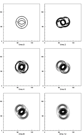
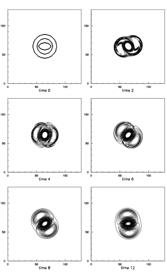
da-Evolution of the unperturbated state: 256 modes
Evolution of the perturbated state: 256 modes
tum any bounded measurable functionω0(x)and we define: ω(t,x)=ω0
ϕ−1 t (x)
(i.e.ωis merely transported byϕt). Thenu(t, x)is defined by:
∇×u=ω, ∇·u=0, u·n=0 on ∂. (4)
Our system is a kind of altered Euler equation, where the dependency betweenϕanduis broken but which keeps the property of yielding vorticity oscillations at smaller and smaller spatial scales.
4.2 Properties of the model Let us denoteω0 = ||−1
ω0(x) dx, the mean value of the initial vorticity function. Due to the mixing assumption onϕt, one can easily prove that:
ω(t,x)→ω0 ast→ ∞, in a weak sense,
i.e.ω(t,x)θ(x) dx→ω0θ(x) dx, for any continuous functionθdefined on.
Then it follows from (4), by a standard compactness argu-ment, that:
u(t,x)−u0(t,x)2
dx→0 ast→ ∞,
whereu0is defined by∇×u0=ω0, ∇·u0=0, u0·n= 0 on ∂.
Thus we see that for this simple system the mixing prop-erty ofϕimplies the strong (in the energy norm) convergence ofu(t,x)towardsu0. Let us suppose, for instance, that is a disk, then ast → ∞, the velocity field will converge towards a solid body rotation.
Although more intricate the situation is similar for Eu-ler equations; to get EuEu-ler system one only has to add the relationship ∂ϕ
∂t (t,x) = u
t,ϕ(t,x). Of course the La-grangian flowϕ(t, x)is no more mixing, due to conservation of the energy; nevertheless some “chaotic” feature remains as Arnold’s calculations and numerical simulations show (Car-ton and Legras, 1994; Robert and Rosier, 1997; Sommeria et al, 1991).
Thus the appearance of coherent structures is caused by the mixing property of the Lagrangian flow. And we may say that for Euler equations (as for the simplified model) it is the unpredictability of the Lagrangian flow which makes the long time prediction of the velocity field eventually possible. To conclude, the above considerations suggest that, for two-dimensional fluid motion, the long time prediction might be possible as far as we can describe the motion in terms of the velocity fieldu(t, x). This suggestion will be investigated in the following section.
4.3 Remarks
Remark 1: It was suggested by Onsager that the formation of the coherent structures might be described in terms of sta-tistical mechanics.But every stasta-tistical mechanics approach relies on some ergodic assumption; in the approach given by (Miller et al., 1992; Robert, 1991; Robert and Sommeria, 1991) the Lagrangian flow is supposed to be as mixing as possible within the constraints given by the constants of the motion. The fact that the predictions of this statistical the-ory have been verified precisely in many cases (Robert and Rosier, 1997; Sommeria et al, 1991) shows that this assump-tion is reasonable, at least in the turbulent areas of the flow.
Remark 2: The mechanism of violent relaxation described above is typically related to the infinite dimensional feature of the problem. The vorticity function oscillates at smaller and smaller spatial scales, involving an infinite number of degrees of freedom. To perform numerical simulations we will truncate our system into a D dimensional one and we expect to observe different behaviors according to the order of magnitude of D. This point will be addressed in the fol-lowing section.
5 Numerical simulations
Now we will test the theoretical considerations of the previ-ous sections on a well known example: the formation of a tripolar coherent structure.
Such structures are composed of three juxtaposed vortices, a central vortex surrounded by two satellite counterrotating vortices, the whole structure moving with a uniform rota-tional motion. Tripolar structures can be observed in the at-mosphere or the oceans; they can also be obtained in labo-ratory experiments or, even more easily, by numerical simu-lations (Carton and Legras, 1994; Robert and Rosier, 1997; Van Heijst et al, 1991). We choose this example because it is a well defined structure which can split into two dipoles when it is subjected to a perturbation ; this allows us to get interesting effects from the stability point of view.
5.1 Description of the numerical simulations
As usual, we will approximate the flow in the whole plane by taking an initial datum localized in a small portion of a (comparatively) large periodic domain=]0,2π[×]0,2π[.
The initial vorticity function is defined as follows:
ω0(x)=a1in the ellipse (x1−π)
2
r02 + (x2−π)2
r12 ≤
1,
ω0(x)=a2in the annulusr22≤(x1−π)2+(x2−π)2≤r32,
ω0(x)=0 elsewhere.
Due to the periodicity of the flow in the two directions, the mean value ofω0onmust vanish, so that the parameters
a1, a2, r0, r1, r2, r3satisfya1r0r1=a2(r22−r32).
In what follows, we will take: a2 = 2π,r0 = 0.5,r1 = 0.3,r2=0.65,r3=1 (or 0.9325).
For the needs of numerical computation we introduce a small viscosity νe = 1/Re and we solve numerically, in a classical way, the Navier-Stokes equations with periodic boundary conditions. The spatial derivatives are treated by a pseudo-spectral method, and the time discretization scheme is a third order Adams-Bashforth scheme.
5.2 First simulation, formation of a tripolar structure In this first simulation, we simply observe the formation of the tripolar structure (Robert and Rosier, 1997).
5.2.1 Numerical parameters
(i) Spatial resolution: the highest spatial resolution is of course desirable in order to reach high Reynolds number and properly handle the initial vorticity discontinuity. We chose
N = 256, that is to say a grid of 256×256 points; this will allow us to approach the inertial limit with a reasonable computing time.
(ii) Reynolds number: We take Re= 2000, which is the highest Reynolds number compatible with our resolution.
(iii) Time step:t =0.001. 5.2.2 The results
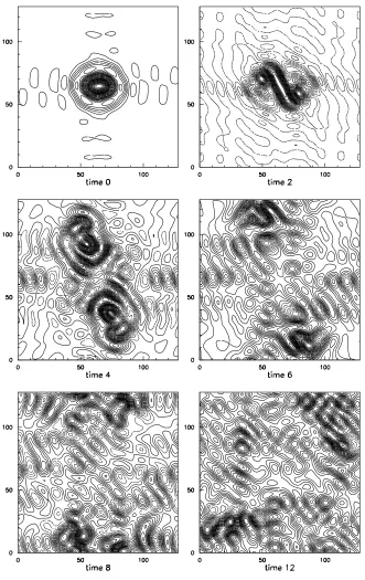
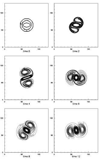
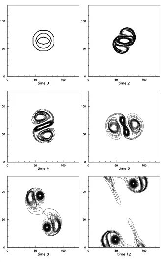
Forr3 = 1, the simulated flow is described in Fig. 1a: the evolution of the flow is represented by successive snapshots of the vorticity field at different times. We see the intricate motion of the fluid yielding the mixing of the vorticity lev-els 0, a1, a2. After this mixing process, the system stabilizes into a tripolar vortex structure which only slowly diffuses by viscosity. In the final state, the system has a steady configura-tion in a rotating reference frame (Robert and Rosier, 1997). If we continuously decreaser3, the same behavior takes place until a critical value is reached, approximately equal to 0.9325; below this value the system does not converge towards a tripole but splits into two dipoles (see Fig. 4b). 5.3 Second simulation: effect of a small perturbation of the
initial datum
The perturbation of the initial vorticity (caser3=1) is taken as proportional to the eigenvector associated with the greatest eigenvalue of the linearized operator. The energy norm of the perturbation is equal to 1% of the energy norm of the initial datum.
5.3.1 The results
At first sight (see Fig. 1b) we don’t see any appreciable dif-ference to the unperturbed flow (Fig. 1a). If we observe the small scale motion, of course one can see changes, but at large scale the flow seems unchanged by the perturbation.
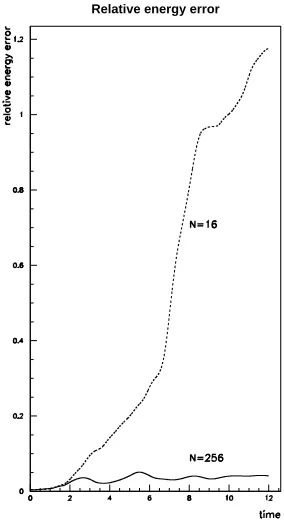
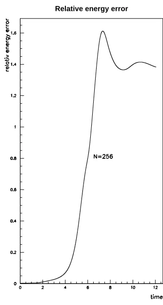
Now, let us draw the curve giving the time evolution of the relative error in energy norm (Fig. 2,N =256):
e(t)= u(t,x)−up(t,x)
2
dx u(t,x)2dx
1/2
,
Relative energy error
Fig. 2. Relative energy error: (r3 = 1),N = 16 (dotted line), N=256, e=0.01.
whereup(t,x)is the perturbed velocity field. One can see a phase of exponential growth ofe(t)which is relatively short (of the order of magnitude of a few turning times of the struc-ture) and then after some weak oscillationse(t)stabilizes at a value which is about 0.04.
5.4 Third simulation, changing the number of degrees of freedom
We perform exactly the same computations with the only pa-rameter changed being the number of degrees of freedom
D=N2.
5.4.1 The results
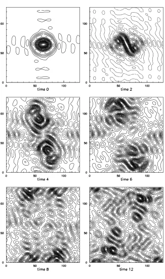
Now forN =16, we no longer observe the formation of a structure and the “chaotic” oscillations of the vorticity func-tion fill the periodic box (Fig. 3a).
We notice that the influence of the initial perturbation, which is hardly visible for t = 2, progressively contami-nates all the scales of the flow (Fig. 3b). This appears clearly on the error diagrame(t)(Fig. 2,N = 16), where we see that, contrary to the caseN = 256, the relative error does not remain small.
5.4.2 Remark
ap-Evolution of the unperturbated state: 16 modes
Evolution of the perturbated state: 16 modes
Evolution of the unperturbated state: 256 modes
Evolution of the perturbated state: 256 modes
proximation of the Navier-Stokes equations. But this does not matter since our purpose is to show the variation of the behavior of the discretized dynamical system with the num-ber of degrees of freedom and not to test its adequacy for the Navier-Stokes equations, which can only appear for largeN. 5.5 Fourth simulation, initial datum about a separatrix We perform again the same computations but with an initial datum about the critical radius 0.9325.
5.5.1 The results
A first calculation withr3=0.9325 still displays the forma-tion of a tripolar structure (Fig. 4a).
We add a small perturbation to the initial vorticity, in fact we taker3 = 0.9320 (which corresponds to a relative error in energy norm of 0.0029). We see that up tot =4 the evo-lution is quite unchanged, then suddenly the central vortex splits into two vortices and afterwards the whole structure splits into two dipoles (Fig. 4b).
The time evolution of the errore(t)(Fig. 5) now shows clearly an exponential sensitivity during the splitting into two dipoles.
5.6 Comments on the numerical experiments
The second and third simulations show that, for a large num-ber of degrees of freedom, the stage of exponential error growth lasts only a few turning times. Although the sys-tem is very unstable, the perturbation mainly affects the small scales and has a very small influence on the large-scale mo-tion. This is the case when the system tends to form a well defined coherent structure.
The fourth simulation shows that the exponential sensitiv-ity, with respect to the initial datum, can persist at longer range if we start on a “separatrix” between two different possibilities of large-scale coherent structures. The system can then converge towards one structure or another. This can drastically change the large scale motion because we are close to a phase transition and a small perturbation of the constants of the motion (energy, enstrophy...) can change the statistical equilibrium (see Robert-Sommeria, 1991).
6 Conclusion
To conclude, our simulations clearly show that Lorenz’s pic-ture of a small local perturbation of the atmosphere, which progressively increases and gains larger and larger scales by nonlinear interaction and finally causes a significant large-scale change in the atmospheric flow, is a misleading descrip-tion of the nonlinear stage of evoludescrip-tion. When a large number of degrees of freedom are involved a new nonlinear process is at work leading to the formation of the coherent structures and this can improve the long range predictability prognosis for large scale motion. Nevertheless, we notice that Lorenz’s
Relative energy error
Fig. 5. Relative energy error:r3=0.9325,N=256, e=0.0029.
scenario accurately describes the exceptional case where we start on a “separatrix”.
A study of the error propagation based on a statistical mod-eling of two-dimensional turbulence yields a relative energy error of the form (Lesieur, 1990):
r(t)=r(0)exp t
τ0
,
whereτ0is the turning time of the large eddies (about 1 day for the terrestrial atmosphere) anda constant with approx-imate values 2.6 for the stationary turbulence and 4.8 for the freely decreasing case. Such a formula can account for the increasing phase of the error during a few turning times but it cannot account for the observed error at longer times in the simulations (Fig. 2).
On the other hand, even if the thermodynamic parametriza-tion of the small scales is appropriately done, it would still be necessary to compute the evolution of a system composed of a finite number of structures which is something like a dy-namical system composed of a few point vortices in which behavior can be chaotic (in the case of 3 point vortices we know that that the system is integrable thus predictable but for 4 point vortices it was shown that it has a chaotic behav-ior (Aref and Pomphrey, 1980; Koiller and Carvalho, 1989; Ziglin, 1980)).
Acknowledgements. The authors are grateful to Olivier Talagrand for kindly giving them relevant references on the atmospheric pre-dictability problem.
References
Aref, H. and Pomphrey, N., Integrable and chaotic motions of four vortices, Physics Letters, 78 A, No. 4, 297–300, 1980.
Arnold, V. I., Sur la g´eom´etrie diff´erentielle des groupes de Lie de dimension infinie et ses applications `a l’hydrodynamique des flu-ides parfaits, Annales de l’Institut Fourier, XVI, No. 1, 319–361, 1966.
Arnold, V. I., Les m´ethodes math´ematiques de la m´ecanique clas-sique, Ed. Mir., 1976.
Carton, X. and Legras, B., The life cycle of tripoles in two-dimensional incompressible flows, J. Fluid Mech., 267, 53–82, 1994.
Chavanis, P. H., Sommeria, J., and Robert, R., Statistical mechan-ics of two-dimensional vortices and collisionless stellar systems, The Astrophysical Journal, 471, 385–399, 1996.
Farrell, B. F., Small error dynamics and the predictability of atmo-spheric flows, J. Atmos. Sci., 47, No. 20, 2406–2416, 1990. Klinker, E., Rabier, F., and Gelaro, R., Estimation of key analysis
errors using the adjoint technique, Q. J. R. Meteorol. Soc., in press.
Koiller, J. and Carvalho, S. P., Non-integrability of the 4-Vortex System: Analytical proof, Comm. Math. Phys., 120, 643–652, 1989.
Leith, C. E., Numerical simulation of the earth’s atmosphere, in Methods in Computational Physics, Vol 4, Academic Press, New York, 1–28, 1965.
Leith, C. E., Objective methods for weather prediction, Ann. Rev. Fluid Mech., 10, 107–128, 1978.
Lesieur, M., Turbulence in fluids, 2nd edn., Kluwer, 1990. Lorenz, E. N., Deterministic nonperiodic flow, J. Atmos. Sci., 20,
130–141, 1963.
Lorenz, E. N., A study of the predictability of a 28-variable atmo-spheric model, Tellus, 17, 321–333, 1965.
Lorenz, E. N., The predictability of a flow which possesses many scales of motion, Tellus, 21, 289–307, 1969.
Lorenz, E. N., Atmospheric predictability experiments with a large numerical model, Tellus, 34, 505–513, 1982.
Lybden-Bell, D., Statistical mechanics of violent relaxation in stel-lar systems, Mon. Not. R. Astr. Soc., 181, 405, 1967.
Miller, J., Weichman, P. B., and Cross, M. C., Statistical mechanics, Euler equations, and Jupiter’s red spot, Phys. Rev. A, 45, 2328– 2359, 1992.
Onsager, L., Statistical hydrodynamics, Nuovo Cimento Supp., 6, 279, 1949.
Rabier, F., Klinker, E., Courtier, P., and Hollingsworth, A., Sensi-tivity of forecast errors to initial conditions, Q. J. R. Meteorol. Soc., 122, 121–150, 1996.
Robert R., A maximum entropy principle for two-dimensional Euler equations, J. Stat. Phys., 65, 3/4, 531–553, 1991.
Robert, R. and Sommeria, J., Statistical equilibrium states for two-dimensional flows, J. Fluid Mech., 229, 291–310, 1991. Robert, R. and Rosier, C., On the modelling of small scales for 2D
turbulent flows, J. Stat. Phys., 86, 3/4, 1997.
Smagorinsky, J., General circulation experiments with the primitive equations, I. The basic experiment, Mon. Wea. Rev., 91, 99–164, 1963.
Smagorinsky, J., Problems and promises of deterministic extended range forecasting, Bull. Amer. Meteorol. Soc., 50, 286–311, 1969.
Sommeria, J., Staquet, C., and Robert, R., Final equilibrium state of a two-dimensional shear layer, J. Fluid Mech., 233, 661–689, 1991.
Van Heijst, G. J. F., Kloosterziel, R. C., and Williams, C. W. M., Laboratory experiments on the tripolar vortex in a rotating fluid, J. Fluid Mech., 225, 301–331, 1991.
Youdovitch, V. I., Non-stationary flow of an incompressible liquid, Zh. Vych. Mat., 3, 1032–1066, 1963.