https://doi.org/10.5194/amt-10-3833-2017 © Author(s) 2017. This work is distributed under the Creative Commons Attribution 3.0 License.
Airborne DOAS retrievals of methane, carbon dioxide, and
water vapor concentrations at high spatial resolution:
application to AVIRIS-NG
Andrew K. Thorpe1, Christian Frankenberg2,1, David R. Thompson1, Riley M. Duren1, Andrew D. Aubrey1, Brian D. Bue1, Robert O. Green1, Konstantin Gerilowski3, Thomas Krings3, Jakob Borchardt3, Eric A. Kort4, Colm Sweeney5, Stephen Conley6,7, Dar A. Roberts8, and Philip E. Dennison9
1Jet Propulsion Laboratory, California Institute of Technology, Pasadena, California, USA
2Division of Geological and Planetary Sciences, California Institute of Technology, Pasadena, California, USA 3Institute of Environmental Physics (IUP), University of Bremen, Bremen, Germany
4Department of Climate and Space Sciences and Engineering, University of Michigan, Ann Arbor, Michigan, USA 5Cooperative Institute for Research in Environmental Sciences, University of Colorado, Boulder, Colorado, USA 6Global Monitoring Division, NOAA Earth System Research Laboratory, Boulder, Colorado, USA
7Scientific Aviation, 3335 Airport Road, Boulder, Colorado, USA
8Department of Geography, University of California, Santa Barbara, Santa Barbara, California, USA 9Department of Geography, University of Utah, Salt Lake City, Utah, USA
Correspondence to:Andrew K. Thorpe ([email protected])
Received: 18 February 2017 – Discussion started: 9 May 2017
Revised: 29 August 2017 – Accepted: 5 September 2017 – Published: 19 October 2017
Abstract.At local scales, emissions of methane and carbon dioxide are highly uncertain. Localized sources of both trace gases can create strong local gradients in its columnar abun-dance, which can be discerned using absorption spectroscopy at high spatial resolution. In a previous study, more than 250 methane plumes were observed in the San Juan Basin near Four Corners during April 2015 using the next-generation Airborne Visible/Infrared Imaging Spectrometer (AVIRIS-NG) and a linearized matched filter. For the first time, we apply the iterative maximum a posteriori differential optical absorption spectroscopy (IMAP-DOAS) method to AVIRIS-NG data and generate gas concentration maps for methane, carbon dioxide, and water vapor plumes. This demonstrates a comprehensive greenhouse gas monitoring capability that targets methane and carbon dioxide, the two dominant an-thropogenic climate-forcing agents. Water vapor results in-dicate the ability of these retrievals to distinguish between methane and water vapor despite spectral interference in the shortwave infrared. We focus on selected cases from anthro-pogenic and natural sources, including emissions from mine ventilation shafts, a gas processing plant, tank, pipeline leak, and natural seep. In addition, carbon dioxide emissions were
mapped from the flue-gas stacks of two coal-fired power plants and a water vapor plume was observed from the com-bined sources of cooling towers and cooling ponds. Observed plumes were consistent with known and suspected emis-sion sources verified by the true color AVIRIS-NG scenes and higher-resolution Google Earth imagery. Real-time de-tection and geolocation of methane plumes by AVIRIS-NG provided unambiguous identification of individual emission source locations and communication to a ground team for rapid follow-up. This permitted verification of a number of methane emission sources using a thermal camera, including a tank and buried natural gas pipeline.
1 Introduction
It is important to better understand the processes control-ling changes in atmospheric methane (CH4) and carbon
diox-ide (CO2), the two dominant anthropogenic climate-forcing
agents. CH4and CO2contribute approximately 17 and 64 %
greenhouse gases and halocarbons (Myhre et al., 2013). The atmospheric growth rates are strongly influenced by anthro-pogenic emissions of CH4and dominated by fossil fuel CO2
emissions. Anthropogenic CH4 sources were estimated to
contribute 10.6 % of the total 2014 anthropogenic emissions of the United States, with major sources including natural gas systems (2.6 %), enteric fermentation (2.4 %), landfills (2.2 %), petroleum systems (1.0 %), and coal mining (1.0 %) (EPA, 2016a). CH4is a precursor for tropospheric ozone and
is strongly linked with co-emitted reactive trace gases that are the focus of air quality mitigation policies. US anthropogenic CO2sources make up 81 % of the total anthropogenic
emis-sions and are dominated by fossil fuel combustion, includ-ing electricity generation (30 %), transportation (25 %), and industrial emissions (12 %) (EPA, 2016a). US emissions of both gases are projected to increase (EIA, 2013) and a num-ber of studies have suggested that EPA bottom-up emission inventories are underestimated for CH4(Miller et al., 2013;
Wecht et al., 2014; Turner et al., 2015). US fossil fuel CO2
emissions are better constrained through existing inventories of fossil fuel sales and combustion, but global uncertainties are growing with the rise of a number of large developing countries where emissions information is not readily avail-able (NRC, 2010; Ballantyne et al., 2015; Ciais et al., 2015). There remains uncertainty regarding the sources and sinks of atmospheric CH4, as reflected by the ongoing scientific
discussion on both the hiatus in the atmospheric growth rate in the early 21st century and the unexpected rise starting in 2007 (Nisbet et al., 2014). Further, regional top-down emis-sions estimates cannot discriminate source categories and thereby attribute fluxes to specific processes or sources. Un-certainty in anthropogenic CH4emissions is large at multiple
scales and process attribution remains challenging because emissions originate from biological processes, venting, and leaks (Kirschke et al., 2013; Schwietzke et al., 2016; Schae-fer et al., 2016).
Recent studies suggest that the majority of CH4
emis-sions from oil and gas supply chains are caused by a num-ber of super-emitters, which could explain underestimates in bottom-up inventories (Zavala-Araiza et al., 2015; Lyon et al., 2015; Brandt et al., 2014, 2016). The ability to identify emission sources offers the potential to constrain regional greenhouse gas budgets and improve partitioning between anthropogenic and natural emission sources. Although CH4
has a short atmospheric lifetime (about 9 years), it has a very high global warming potential (GWP) that is 86 times greater than CO2on a 20 year timescale (Myhre et al., 2013). This
means that even small amounts of emissions reduction will result in large reductions in the overall atmospheric radiative forcing.
Driving surveys using in situ instruments have been used to identify CH4 emission sources in major US
metropoli-tan areas like the Los Angeles basin (Hopkins et al., 2016), Boston (Phillips et al., 2013), and Washington, D.C. (Jackson et al., 2014), as well as to measure fluxes (Rella et al., 2015).
Recently, ground-based thermal imaging systems have also been used to identify CH4emissions (Johnson et al., 2015;
Galfalk et al., 2016). However, these methods require com-prehensive sampling techniques, are time consuming, and can be limited to regions with sufficient road access. In situ airborne measurements offer the potential for increased cov-erage and have been used for US regional CH4flux estimates
using mass balance approaches for the Uintah Basin in north-eastern Utah (Karion et al., 2013), the Marcellus formation in southwestern Pennsylvania (Caulton et al., 2014), and the Barnett Shale formation in Texas (Smith et al., 2015; Lavoie et al., 2015). These measurements reflect gas concentrations at the flight altitude and these studies are designed to estimate aggregate emissions for large regions rather than identifying individual emissions sources.
More recently, in situ airborne measurements using a chemically instrumented Mooney aircraft have been used to estimate fluxes from known sources like the Aliso Canyon leak (Conley et al., 2016) and for a number of sources iden-tified by imaging spectrometers in the Four Corners region (Frankenberg et al., 2016). This method samples the at-mosphere directly at the flight path altitude and can mea-sure multiple gas species. The Methane Airborne MAPper (MAMAP) spectrometer (Gerilowski et al., 2011) has also been used to measure elevated CH4and CO2column
abun-dances to quantify emissions from a coal mine ventilation shaft (Krings et al., 2013), power plants (Krings et al., 2011), and a landfill (Krautwurst et al., 2017). MAMAP is a non-imaging spectrometer with a small field of view limited to flying transects across gas plumes rather than quickly map-ping their morphology and extent on small scales. Both in-struments are better suited for either investigating known emission sources or identifying larger regional emissions as opposed to individual sources.
2 Airborne imaging spectrometers
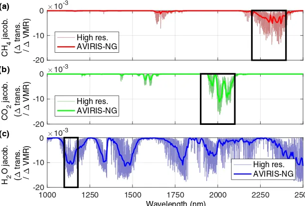
Airborne imaging spectrometers like the Airborne Visi-ble/Infrared Imaging Spectrometer (AVIRIS) (Green et al., 1998) and the next-generation instrument AVIRIS-NG (Hamlin et al., 2011) can map large regions while pro-viding the spatial resolution required to identify individual emissions within scenes. While not originally designed for mapping emissions, these instruments measure the 0.38 to 2.5 µm range, which includes many gas absorption features (Fig. 1). This has permitted quantitative retrievals of CH4
appli--20 -10 0 CH 4 jacob. ( " tr a n s. / " VMR)
#10-3
(a) High res. AVIRIS-NG -20 -10 0 CO 2 jacob. ( " tr a n s. / " VMR)
#10-3
(b)
High res. AVIRIS-NG
1000 1250 1500 1750 2000 2250 2500
Wavelength (nm) -20 -10 0 H 2 O jacob. ( " tr a n s. / " VMR)
#10-3
(c)
High res. AVIRIS-NG
Figure 1.High-resolution gas Jacobians plotted in lighter colors and for AVIRIS-NG (5 nm spectral resolution and sampling) for(a)CH4 (red),(b)CO2(green), and(c)H2O (blue). These examples were calculated for a 5 % change in CH4(red),(b)CO2(green), and(c)H2O over the total column. AVIRIS-NG retrieval windows are indicated by the black outlines.
Source: Esri, DigitalGlobe, GeoEye, Earthstar Geographics, CNES/Airbus DS, USDA, USGS, AeroGRID, IGN, and the GIS User Community 106°0'0" W 106°0'0" W 107°0'0" W 107°0'0" W 108°0'0" W 108°0'0" W 109°0'0" W 109°0'0" W 110°0'0" W 110°0'0" W 111°0'0" W 111°0'0" W 40 °0 '0 "N 40 °0 '0 "N 39 °0 '0 "N 39 °0 '0 "N 38 °0 '0 "N 38 °0 '0 "N 37 °0 '0 "N 37 °0 '0 "N 36 °0 '0 "N 36 °0 '0 "N 35 °0 '0 "N Legend
Fig. 3: CH4 Fig. 6: CH4 Fig. 7: CO2 Fig. 9: CH4 Fig. 10: CH4 Fig. 11: CH4 Fig. 12: CO2, H2O
0 50 100 200 300km
Colorado
New Mexico
Utah
Arizona
Figure 2.Locations of gas plumes presented in this study.
cation to the fields of ecology and meteorology (Ogunjemiyo et al., 2002).
AVIRIS has been used for high-resolution mapping of CO2plumes from industrial sources (Dennison et al., 2013)
and wildfires (Marion et al., 2004; Deschamps et al., 2011). More recently, AVIRIS-NG (approximately 5 nm spectral resolution and sampling) has surveyed large regions to iden-tify CH4emissions associated with oil production
(Thomp-son et al., 2015b), gas extraction (Frankenberg et al., 2016),
hydraulic fracturing (Aubrey et al., 2015), and a landfill (Krautwurst et al., 2017). This is possible due to a 34◦field of view, which results in an image swath of 1.8 km when flying at 3 km a.g.l.(above ground level).
Airborne imaging spectrometers that operate in the ther-mal infrared, such as the Mako and HyTES instruments (Tratt et al., 2014; Hulley et al., 2016), have also been used for mapping CH4plumes. However, the altitude of maximum
sensitivity varies with environmental conditions like thermal contrast (Kuai et al., 2016), which can make plumes diffi-cult to detect and quantify, and sensitivity to near-surface emissions decreases with flight altitude, which can limit ground coverage. Because AVIRIS and AVIRIS-NG mea-sure reflected solar radiation in the shortwave infrared, CH4
retrieval sensitivity is impacted only slightly by flight alti-tude due to additional gas attenuation along the optical path. However, at higher flight altitude and coarser spatial resolu-tion a gas enhancement is diluted over a larger image pixel, thereby decreasing instrument sensitivity. The ability to fly high results in more efficient flight campaigns due to im-proved ground coverage. For example, AVIRIS-NG consis-tently observed plumes for a CH4controlled release
experi-ment for all altitudes flown (up to 3.8 km a.g.l.) and AVIRIS has observed CH4 plumes flying at 8.9 km a.g.l. (Thorpe
et al., 2014). AVIRIS has also mapped CH4plumes over
mul-tiple days from the Aliso Canyon leak by flying 6.6 km a.g.l., resulting in an image swath approximately 4.0 km wide (Thompson et al., 2016). This also offers the potential for space-based detection of emission sources, like the observed CH4 plume from Aliso Canyon using the orbital Hyperion
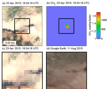
Figure 3. (a)AVIRIS-NG true color image subset.(b)A number of CH4plumes are clearly visible with maximum enhancements in excess of 5000 ppm·m.(c)Close-up of AVIRIS-NG true color image shown by black outline in(a).(d)Higher-resolution Google Earth imagery for same area reveals drilling rigs at an active underground coal mine, suggesting that the origin of these plumes is mine workings ventilation shafts.(e)H2O retrieval does not indicate enhancements. For all images, north is up.
In a previous study (Thorpe et al., 2014), the iterative maximum a posteriori differential optical absorption spec-troscopy (IMAP-DOAS) retrieval was applied to AVIRIS for quantitative mapping of CH4from natural and anthropogenic
sources. In this study, the application of IMAP-DOAS has been expanded for use with AVIRIS-NG for multiple gas species, including CH4, CO2, and H2O. We present results
from AVIRIS-NG data acquired in New Mexico and Col-orado, including from a flight campaign in the San Juan Basin near Four Corners. We will present results for a num-ber of sources, including CH4from mine ventilation shafts,
a gas processing plant, tank, pipeline leak, and natural seep, as well as CO2and H2O plumes associated with power plants
(Fig. 2).
3 Study sites and AVIRIS-NG data
Space-based observations collected by the SCanning Imag-ing Absorption SpectroMeter for Atmospheric CHartogra-phY (SCIAMACHY) instrument (Bovensmann et al., 1999) showed CH4enhancements in the Four Corners region (Kort
et al., 2014). This made for an ideal location for follow-up
0.1 0.15 0.2 0.25 0.3 0.35
Radiance
(
7
W
c
m
-2
n
m
s
r)
(a)
Meas. Model
(b)
2200 2250 2300 2350 2400 Wavelength (nm) -0.01
0 0.01 0.02
Residual
(
7
W
c
m
-2
n
m
s
r)
1 < SD
0 0.5 1 1.5 2 2.5 Radiance ( 7 W c m -2 n m s r) (a) Meas. Model (b)
1100 1120 1140 1160 1180 Wavelength (nm) -0.075 0 0.075 0.15 Residual ( 7 W c m -2 n m s r)
1 < SD
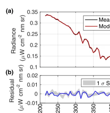
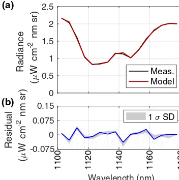
Figure 5. (a)AVIRIS-NG measured and modeled radiance for one image pixel within the CH4plume used for the H2O retrieval (see Fig. 3e).(b)The residual is plotted with 1σSD boundary calculated from residuals for the entire scene.
surveys using AVIRIS-NG to identify individual emission sources. During the flight campaign, the AVIRIS-NG instru-ment was equipped with a real-time CH4mapping capability
using a waterfall display monitored by the instrument opera-tor. Observed CH4plumes were overlaid on a true color
im-age displaying location information and the maximum CH4
enhancement (Thompson et al., 2015b). This permitted adap-tive survey strategies to investigate observed plumes and the ability to send images of the plume with accurate loca-tions to a ground crew for subsequent follow-up. A Xen-ics Onca-VLWIR-MCT-384 thermal imaging camera with a Spectrogon optical filter centered at 7.746 µm was used by the ground crew to verify a number of plumes observed in real time by AVIRIS-NG.
Located in New Mexico and Colorado, the San Juan Basin produces natural gas from sandstone, coal bed CH4, and
shale formations and is the fourth largest US gas field when it comes to total production (EIA, 2015). During a 5-day campaign in April 2015, AVIRIS-NG targeted an area cor-responding to the highest CH4enhancements observed with
SCIAMACHY (Frankenberg et al., 2016). A 2500 km2area was covered in approximately 2 days (9.2 flight hours) fly-ing at 3 km a.g.l., resultfly-ing in scenes with an image swath of around 1.8 km and a ground resolution of 3 m. The re-maining flight days were used for additional follow-up flights and some repeat observations, sometimes at lower flight al-titudes. During the campaign, a number of potential CH4
emission sources were targeted, including infrastructure as-sociated with natural gas production like well pads, tanks, gas processing plants, a coal mine, and natural coal bed CH4
seeps. While the flight campaign focused on CH4 sources,
the coal-fired San Juan power-generating station was also flown as a potential CO2emission source.
4 IMAP-DOAS retrievals
A detailed description of the IMAP-DOAS retrieval for AVIRIS can be found in Thorpe et al. (2014). Gas retrievals were performed on orthocorrected radiance data. Atmo-spheric profiles were generated by updating prior gas profiles from the US standard atmosphere obtained from the radiative transfer models LOWTRAN/MODTRAN (Kneizys et al., 1996) using volume mixing ratios (VMRs) from the NOAA Mauna Loa station, United States (NOAA, 2015). Tempera-ture, pressure, and water vapor VMR profiles representative of the time period of the flight campaign were acquired from the National Centers for Environmental Prediction/National Center for Atmospheric Research (NCEP/NCAR) reanalysis project (Kalnay et al., 1996). Spectral parameters for CH4,
CO2, H2O, and N2O were used from the HITRAN 2008
database (Rothman et al., 2009) and a classical Voigt spec-tral line shape was used to calculate vertical optical densities for 14 atmospheric layers that spanned sea level to the top of the atmosphere.
Above the aircraft, vertical optical densities were com-bined and an air mass factor (AMF) was calculated to ac-count for one-way transmission. Vertical optical densities be-low the aircraft were also combined with an AMF reflect-ing two-way transmission. This resulted in a two-layer atmo-spheric model that speeds up the retrieval and incorporates the ground elevation and flight altitude for each AVIRIS-NG scene. The two-layer model was used to model reflected so-lar radiation perturbed by the absorbing species CH4, CO2,
H2O, and N2O. Three retrieval windows were used, each
tar-geting the primary gas of interest. CH4 retrievals were
per-formed between 2215 and 2410 nm (Fig. 1) and included fits for H2O and N2O. Gas Jacobians that reflect changes
in absorption due to the absorbing species CH4, CO2, and
H2O are shown in Fig. 1. Because N2O has weak
absorp-tion features, these Jacobians are not shown. Between 1904 and 2099 nm, CO2retrievals included H2O and N2O as
ad-ditional unknown variables of the retrieval, while H2O
re-trievals between 1103 and 1178 nm also included CO2 and
N2O. Therefore, the state vector (xn) for each retrieval win-dow has six entries (three gases for two atmospheric layers). Modeled radiance at high spectral resolution was calculated for each wavelength with a forward radiative transfer model using the following equation:
Fhr(xi)=Ihr0 ·exp − 6 X
n=1
An·τrefn ·xn,i !
· k X
i=0
akλk, (1)
is the trace-gas-related state vector at theith iteration, which scales the prior optical densities of each of the absorbing species in eachnlayer (six rows, three gases for two atmo-spheric layers); andakare polynomial coefficients to account for low-frequency spectral variations.
The state vector contains the spectral shift (not shown here) and a low-order polynomial function (ak) to account for the broadband variability in surface albedo (see Franken-berg et al., 2005). The high-resolution modeled radiance is convolved using the instrument line shape function and sam-pled to the center wavelengths for each AVIRIS-NG spec-tral band, resulting in a lower-resolution modeled radiance at theith iteration of the state vectorFlr(x
i), calculated using a knownτref
n scaled byxn,i.
A Jacobian matrix is calculated for each iterationi, where each column represents the derivate vector of the sensor ra-diance with respect to each element of the state vector (xi).
Ki=
∂Flr(x) ∂x x i (2)
The state vector at the ith iteration can be optimized as follows (Rodgers, 2000):
xi+1=xa+
KTi S−ε1Ki+S−a1
−1
KTi S−ε1 ·hy−Flr(xi)+Ki(xi−xa)
i
, (3)
wherexais the a priori state vector (six rows),xi is the state vector at theith iteration (six rows),Sεis the error covariance matrix,Sais the a priori covariance matrix,yis the measured
AVIRIS-NG radiance, Flr(xi)is the forward model evalu-ated at xi, andKi is the Jacobian of the forward model at xi.
The retrieval optimizes a scaling factor relative to the a pri-ori profile. The a pripri-ori scaling factor is set to one as an ini-tial guess for each gas in the two layers, while the a priori covariance matrix was set to constrain the fit to the atmo-spheric layer beneath the aircraft where high variance is ex-pected. To do so, very small prior covariances were set for the uppermost layer (above the aircraft). Because the observed plumes are not expected to extend above the AVIRIS-NG flight altitude, this assumption is reasonable. Gas concen-trations were calculated in ppm·m by multiplying the gas state vector at the last iteration (gas scaling factor) by the VMR for the lowest layer of the reference atmosphere and the distance between the aircraft and the ground. In subse-quent figures, color bars will indicate the scaling factors and gas enhancements relative to background, which were calcu-lated by subtracting the retrieved gas concentration from the background concentration for the lowest layer of the refer-ence atmosphere.
The covariance Sˆ was calculated to estimate expected IMAP-DOAS retrieval errors as follows:
ˆ
S=KTS−ε1K+S−a1 −1
, (4)
where the diagonal of Sˆ corresponds to the covariance at each atmospheric layer associated with the gases used for each fitting window.Sε, the error covariance matrix, is a di-agonal matrix representing expected errors for the retrieval algorithm. For each gas retrieval, the square root of the cor-responding diagonal entry ofSˆis multiplied by the VMR in the lowest layer of the atmospheric model for each retrieved gas (CH4: 1.86 ppm; CO2: 399 ppm; H2O: 7745 ppm).
Us-ing scene parameters for a 1 km flight altitude a.g.l. with 25.6◦solar zenith and variable signal-to-noise ratio, this cor-responds to an error of between 0.14 and 0.55 ppm CH4
be-neath the aircraft. For CO2, the error ranges between 6.6 and
26.4 ppm and for H2O between 9.4 and 37.5 ppm.
5 Results
5.1 CH4emissions from natural gas sector
AVIRIS-NG identified over 250 CH4plumes during the Four
Corners flight campaign (Frankenberg et al., 2016) using a linearized matched filter (Thompson et al., 2015b). The linearized matched filter models the background of radiance spectra as a multivariate Gaussian and provides a scalar value that represents the fraction of the gas target signature that perturbs the background. Because the target signature is de-fined as the change in radiance of the background caused by adding a unit mixing ratio length of CH4, detected quantities
are reported in mixing ratio lengths (ppm·m). This method is computationally efficient and accounts for the full covari-ance of background (atmosphere and surface) and instrument noise using in-scene data, providing high sensitivity to local enhancements.
The current speed of the IMAP-DOAS retrieval algorithm precludes it from being applied to all 250 examples pre-sented in the previous study (Frankenberg et al., 2016). In-stead, IMAP-DOAS retrievals for only a few examples will be presented here, reflecting CH4, CO2, and H2O plumes
from a variety of emission sources. The first example from a 20 April 2015 flight at 1.1 km a.g.l.(Fig. 3b) is made up of at least 10 plumes with maximum enhancements in excess of 5000 ppm m, which is equivalent to a concentration of 0.5 % in a 1 m thick layer or roughly an XCH4 (dry air
column-averaged mole fraction) enhancement of around 500 ppb that is almost 25 % of a total background column. Results from the H2O retrieval (Fig. 3e) do not indicate enhancements
collocated with CH4 plumes. The true color image subset
in Fig. 3a reveals a few dirt roads, but the close-up of the AVIRIS-NG scene indicated by the black boxes in Fig. 3a and b indicates some visible infrastructure that is difficult to interpret at the 1 m AVIRIS-NG pixel resolution (Fig. 3c).
Figure 6. (a)AVIRIS-NG true color image subset.(b)A small CH4plume is visible from a confirmed geological source at Moving Mountain near Durango, Colorado.(c)Close-up of AVIRIS-NG true color image.(d)Higher-resolution Google Earth imagery provides additional spatial context. For all images, north is up.
workings ventilation shafts. Frankenberg et al. (2016) esti-mated an aggregate flux of 2236 kg h−1 for these plumes. Measured and modeled radiance is shown for one image pixel within the CH4plume for the CH4retrieval fitting
win-dow (Fig. 4a) and for the H2O retrieval (Fig. 5a). For both
examples, the residuals are also plotted (Fig. 4b, Fig. 5b) in addition to the 1σSD boundary calculated from residuals for the entire scene.
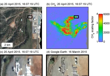
Additional examples are presented in Appendix A, includ-ing from another 20 April 2015 flight at 1.4 km a.g.l.that re-sults in a 1.2 m resolution (Fig. A1b). Multiple CH4plumes
are visible from this gas processing facility, one emanating from a source beyond the east edge of the AVIRIS-NG scene. This example was associated with a planned maintenance op-eration, which resulted in a large temporary CH4plume that
was recorded and reported through the normal Greenhouse Gas Reporting Program (Williams, 2016). A second plume is visible at a location shown by the black box in Fig. A1a, indicating white pipes associated with an interstate pipeline as the likely emission source (Fig. A1c and d).
An H2O retrieval was also performed for this scene
and did not reveal enhancements collocated with the CH4
plumes. For all subsequent examples, H2O retrievals were
performed but will be shown only in cases where H2O
plumes were observed (see Sect. 5.3). As shown in Fig. A1a, the CH4plumes cross over many land cover types with
vari-able brightness and very dark surfaces resulted in anoma-lously high retrievals. CH4results from radiances less than
0.01 µ W cm−2sr−1nm−1 for any band of the CH4 fitting
window, corresponding to shadows and water, were removed from the results shown in Fig. A1b.
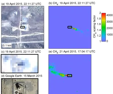
In Fig. A2b and e, CH4emissions from a tank were
ob-served on 19 and 21 April 2015 at 2.8 and 3.2 km a.g.l.(pixel resolutions of 2.6 and 3.0 m respectively). The Google Earth close-up shown in Fig. A2d indicates a tank as the likely emission source, which was confirmed by the ground crew using a thermal imaging camera on multiple days. Video A1 (see Supplement) was acquired on 21 April 2015 at around 18:00 UTC and clearly shows a CH4plume originating at the
top of the tank that is consistent with the AVIRIS-NG CH4
plume observed the same day.
In Frankenberg et al. (2016), CH4 emissions from
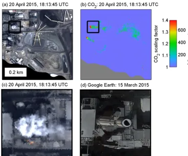
per-Figure 7. (a)AVIRIS-NG true color image subset.(b)CO2plume is visible.(c)Close-up of AVIRIS-NG true color image.(d) Higher-resolution Google Earth imagery provides additional spatial context. For all images, north is up.
0 0.2 0.4 0.6
Radiance
(
7
W
c
m
-2
n
m
s
r)
(a)
Meas. Model
(b)
1900 1950 2000 2050 2100
Wavelength (nm) -0.025
0 0.025 0.05
Residual
(
7
W
c
m
-2
n
m
s
r)
1 < SD
Figure 8. (a) AVIRIS-NG measured and modeled radiance for one image pixel within the CO2plume for the CO2retrieval (see Fig. 7b). (b)The residual is plotted with 1σ SD boundary calcu-lated from residuals for the entire scene.
sonal communication, 2016). That leak was independently identified and repaired by the operator as a part of their nor-mal operations prior to publication. In Fig. A3b, the CH4
plume from the 19 April 2015 flight at 3.0 km a.g.l.(2.7 m pixel resolution) does not appear associated with visible infrastructure and subsequent investigation by the ground crews identified the plume origin on 24 April 2015 using the thermal camera (Video A2, see Supplement). This location was along a marked, buried natural gas pipeline and was sub-sequently confirmed as a pipeline leak and ultimately shut down for repairs by the local pipeline operators. The esti-mated flux for this example is 28 kg h−1(Frankenberg et al., 2016), which would result in an estimated annual loss of 13.2 million cubic feet, equivalent to USD 100 000 (assum-ing constant annual flux and average cost of USD 7.40 per thousand cubic feet).
5.2 Geological CH4emissions
AVIRIS has been used for quantitative retrievals of CH4
source at Moving Mountain near Durango, Colorado (LTE, 2015). This AVIRIS-NG scene was acquired at 1.3 km a.g.l. (1 m pixel resolution) and shows a 10 m long plume (Fig. 6b).
5.3 CO2and H2O emissions from power plants
While Dennison et al. (2013) demonstrated the ability of AVIRIS for high-resolution mapping of CO2plumes, in this
study we present two examples using quantitative retrievals. The first example is from the coal-fired San Juan Generat-ing Station near FarmGenerat-ington, New Mexico, that was flown on 20 April 2015 at 1.2 km a.g.l.Two CO2 plumes are clearly
visible in Fig. 7b and correspond to two flue-gas stacks that appear active given visible emissions in the true color image (Fig. 7a, c). A third flue-gas stack appears inactive (Fig. 7a) with no visible CO2 plume (Fig. 7b). The San Juan
Gen-erating Station reported 2015 emissions of 9843 kt of CO2,
equivalent to a flux of 1 123 666 kg CO2h−1(EPA, 2016b).
An example of a CO2retrieval fit and the residual is shown
in (Fig. 8).
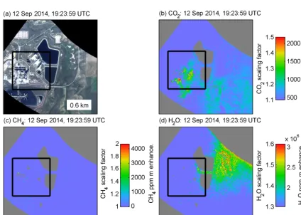
The second example is from a 12 September 2014 flight that included the coal-fired Craig Station near Craig, Colorado. CO2 plumes are visible from flue-gas stacks
(Fig. A4b) and extend more than 1 km downwind. This power plant reported 2014 emissions of 9300 kt of CO2,
equivalent to a flux of 1 061 644 kg CO2h−1(EPA, 2016b).
Within the same scene, an H2O plume is also visible
(Fig. A4d) emanating from a region that contains a num-ber of cooling towers adjacent to two large cooling ponds (Fig. A5a). CH4retrieval results are also shown in Fig. A5c,
indicating that CH4 plumes are not visible in the scene
and emphasizing the ability of these retrievals to distinguish between CH4 and H2O despite spectral interference (see
Fig. 1). Results for dark surfaces like the cooling ponds were removed from Fig. A4b by excluding radiances less than 0.10 µ W cm−2sr−1nm−1 for any band of the CO2 fitting
window, for radiances less than 0.002 µ W cm−2sr−1nm−1 for any band of the H2O fitting window (Fig. A4d), and for
radiances less than 0.01 µ W cm−2sr−1nm−1for any band of the CH4fitting window (Fig. A4c).
In Fig. A5a, the AVIRIS-NG true color image is shown for the close-up indicated by the black box in Fig. A4. The flue-gas stacks are visible in the lower left as CO2
sources and cooling towers in the upper right as possible H2O
sources. Ellipses delineate the shapes of plumes visible in the true color images for the flue-gas stacks (red) and cool-ing towers (blue). The arrows indicate winds to the south-east for the flue-gas stacks (consistent with CO2plumes in
Fig. A4b) and to the east for the cooling towers (consistent with H2O plumes in Fig. A4d). In A5b, the higher-resolution
Google Earth imagery clearly indicates the flue-gas stacks are much taller (182 m) than the cooling tower (TRI, 2016) based on assessment of shadows, which could explain vari-able wind directions at the flue-gas stacks and in the vicin-ity of the cooling towers. Given the presence of the cooling
ponds immediately adjacent to the cooling towers, it is un-clear whether the observed H2O plume shown in Fig. A4d
is caused solely by the cooling towers or reflects the com-bined influence of the towers and evaporation from the cool-ing ponds.
6 Conclusions
In this study, we use the airborne imaging spectrome-ter AVIRIS-NG and the IMAP-DOAS retrieval to generate gas concentration maps for observed CH4, CO2, and H2O
plumes. While more than 250 CH4plumes were observed in
the San Juan Basin near Four Corners (Frankenberg et al., 2016), this study focused on a few results from anthro-pogenic and natural sources, including emissions from mine ventilation shafts, a gas processing plant, tank, pipeline leak, and natural seep. In addition, CO2emissions were observed
from the flue stacks of two coal-fired power plants and an H2O plume was mapped for the cooling towers for one power
plant. Observed plumes were consistent with known and sus-pected emission sources verified by true color AVIRIS-NG imagery and higher-resolution Google Earth imagery.
AVIRIS-NG has the high spatial resolution necessary to resolve small-scale emissions and can map large regions quickly, covering the 2500 km2 Four Corners study in ap-proximately 2 days (9.2 flight hours). This capability is aided by real-time detection and geolocation of gas plumes, per-mitting unambiguous identification of individual emission source locations and communication to ground teams for rapid follow-up. This permitted verification of a number of emission sources presented in this study using a thermal camera, including a tank and buried natural gas pipeline. The AVIRIS and AVIRIS-NG instruments have demon-strated CH4 plume mapping capabilities at multiple flight
altitudes, ranging from as low as 0.4 to 3.8 km a.g.l. (0.4 to 3.8 m pixels) for a controlled release experiment (Thorpe et al., 2016a) to 9 km a.g.l. for the Coal Oil Point marine seeps (Thorpe et al., 2014). AVIRIS observed the Aliso Canyon leak on multiple flight days at 6.6 km a.g.l.(6.6 m pixels) while the Hyperion imaging spectrometer, also 10 nm spectral resolution but 30 m pixels, mapped the plume and demonstrated the potential for a space-based application (Thompson et al., 2016).
This study demonstrates a comprehensive greenhouse gas monitoring capability that targets CH4 and CO2, the two
dominant anthropogenic climate-forcing agents. The ability to identify individual point source locations of CH4and CO2
emissions has relevance to the research community and the private sector. Understanding the spatial and temporal dis-tribution and the magnitude of these emissions is of interest given the large uncertainties associated with anthropogenic emissions. This includes industrial point source emissions of CH4and CO2, CH4from oil and gas operations as well
agricul-tural sources, and CH4and CO2from landfills. Site
opera-tors could identify and mitigate CH4 emissions, which
re-flect both a potential safety hazard and lost revenue. Water vapor results demonstrate the ability of these retrievals to dis-tinguish between CH4and H2O despite spectral interference
in the shortwave infrared while offering the potential to im-prove atmospheric correction and reflectance retrievals with application to the fields of ecology and meteorology.
Despite these promising results, an imaging spectrome-ter built exclusively for quantitative mapping of gas plumes would have improved sensitivity compared to AVIRIS-NG (Thorpe et al., 2014). For example, an instrument provid-ing a 1 nm spectral resolution and samplprovid-ing (2000–2400 nm) would permit mapping CH4, CO2, H2O, CO, and N2O from
more diffuse sources using both airborne and orbital plat-forms (Thorpe et al., 2016b). The ability to identify emission sources offers the potential to constrain regional greenhouse gas budgets and improve partitioning between anthropogenic and natural emission sources. Because the CH4 lifetime is
only about 9 years and CH4 has a high GWP, targeting
re-ductions in anthropogenic CH4emissions offers an effective
approach to decrease overall atmospheric radiative forcing.
Data availability. The AVIRIS-NG data used in this study
Appendix A
This appendix contains additional figures referenced in Sect. 5.
A1 CH4emissions from gas processing facility
A2 CH4emissions from tank
A3 CH4emissions from pipeline leak
A4 CO2and H2O emissions from power plant
Figure A4. (a)AVIRIS-NG true color image subset.(b)CO2plumes are visible emanating from flue-gas stacks.(c)CH4retrieval results. (d)H2O plume visible from cooling towers (see Fig. A5). For all images, north is up.
The Supplement related to this article is available online at https://doi.org/10.5194/amt-10-3833-2017-supplement.
Author contributions. CF and AKT designed research; CF, ADA,
AKT, DRT, BDB, ROG, EAK, CS and SC provided flight campaign support; AKT, CF, DRT, KG, TK and JB performed research; RMD, ROG, KG, TK, JB, DAR and PED advised the research; AKT and CF analyzed data and wrote the paper.
Competing interests. The authors declare that they have no conflict
of interest.
Acknowledgements. The authors thank NASA HQ and Jack Kaye
for funding the flight campaign. We would like to acknowledge the contributions of the AVIRIS-NG flight and instrument teams, including Michael Eastwood, Sarah Lundeen, Ian Mccubin, Mark Helmlinger, Scott Nolte, and Betina Pavri. We would also like to thank Simon Hook and Bill Johnson for their support and for the use of the thermal camera. This work was undertaken in part at the Jet Propulsion Laboratory, California Institute of Technology, under contract with NASA.
Edited by: Andreas Hofzumahaus Reviewed by: two anonymous referees
References
Aubrey, A., Frankenberg, C., Green, R., Eastwood, M., Thomp-son, D., and Thorpe, A.: Crosscutting Airborne Remote Sensing Technologies for Oil and Gas and Earth Sci-ence Applications, Offshore Technology ConferSci-ence, Offshore Technology Conference, 4–7 May, Houston, Texas, USA, https://doi.org/10.4043/25984-MS, 2015.
Ballantyne, A. P., Andres, R., Houghton, R., Stocker, B. D., Wan-ninkhof, R., Anderegg, W., Cooper, L. A., DeGrandpre, M., Tans, P. P., Miller, J. B., Alden, C., and White, J. W. C.: Au-dit of the global carbon budget: estimate errors and their im-pact on uptake uncertainty, Biogeosciences, 12, 2565–2584, https://doi.org/10.5194/bg-12-2565-2015, 2015.
Bovensmann, H., Burrows, J. P., Buchwitz, M., Frerick, J., Noel, S., Rozanov, V. V., Chance, K. V., and Goede, A. P. H.: SCIAMACHY: mission objectives and measurement modes, J. Atmos. Sci., 56, 127–150, https://doi.org/10.1175/1520-0469(1999)056<0127:SMOAMM>2.0.CO;2, 1999.
Brandt, A. R., Heath, G. A., Kort, E. A., O’Sullivan, F., Pétron, G., Jordaan, S. M., Tans, P., Wilcox, J., Gop-stein, A. M., Arent, D., Wofsy, S., Brown, N. J., Bradley, R., Stucky, G. D., Eardley, D., and Harriss, R.: Methane leaks from North American natural gas systems, Science, 343, 733–735, https://doi.org/10.1126/science.1247045, 2014.
Brandt, A. R., Heath, G. A., and Cooley, D.: Methane leaks from natural gas systems follow extreme
dis-tributions, Environ. Sci. Technol., 50, 12512–12520, https://doi.org/10.1021/acs.est.6b04303, 2016.
Caulton, D. R., Shepson, P. B., Santoro, R. L., Sparks, J. P., Howarth, R. W., Ingraffea, A. R., Cambaliza, M. O. L., Sweeney, C., Karion, A., Davis, K. J., Stirm, B. H., Montzka, S. A., and Miller, B. R.: Toward a better under-standing and quantification of methane emissions from shale gas development, P. Natl. Acad. Sci. USA, 111, 6237–6242, https://doi.org/10.1073/pnas.1316546111, 2014.
Ciais, P., Crisp, D., van der Gron, H. D., Engelen, R., Janssens-Maenhout, G., Heimann, M., Rayner, P.„ and Scholze, M.: Towards a European operational observing system to mon-itor fossil CO2 emissions, Final report from the expert group, Tech. Rep., European Comission, Brussels, Bel-gium, http://www.copernicus.eu/sites/default/files/library/CO2_ Report_22Oct2015.pdf, 2015.
Conley, S., Franco, G., Faloona, I., Blake, D. R., Peischl, J., and Ryerson, T. B.: Methane emissions from the 2015 Aliso Canyon blowout in Los Angeles, CA, Science, 351, 1317–1320, https://doi.org/10.1126/science.aaf2348, 2016.
Dennison, P. E., Thorpe, A. K., Pardyjak, E. R., Roberts, D. A., Qi, Y., Green, R. O., Bradley, E. S., and Funk, C. C.: High spatial resolution mapping of elevated atmospheric carbon dioxide using airborne imaging spectroscopy: Radiative transfer modeling and power plant plume detection, Remote Sens. Environ., 139, 116– 129, https://doi.org/10.1016/j.rse.2013.08.001, 2013.
Deschamps, A., Marion, R., Briottet, X., Foucher, P., and Lavigne, C.: Simultaneous CO2 and Aerosol Retrieval in a Vegetation Fire Plume Using AVIRIS Hyperspec-tral Data, 2011 3rd Workshop on. IEEE, Lisbon, Portugal, https://doi.org/10.1109/WHISPERS.2011.6080896, 2011. EIA: US Energy Information Administraton, EIA annual energy
outlook 2013, Tech. rep., US Energy Information Administra-ton, WashingAdministra-ton, DC, United States, available at: https://www. eia.gov/outlooks/aeo/pdf/0383(2013).pdf (last access: 10 May 2017), 2013.
EIA: US Energy Information Administraton, Top 100 US oil and gas fields, Tech. rep., US Energy Information Administraton, U.S. Department of Energy, Washington, DC 20585, avail-able at: https://www.eia.gov/naturalgas/crudeoilreserves/top100/ pdf/top100.pdf (last access: 10 May 2017), 2015.
EPA: US Environmental Protection Agency, Inventory of US Greenhouse Gas Emissions and Sinks: 1990–2014, Technical Report EPA 430-R-16-002 (Environmental Protection Agency), Tech. rep., US Environmental Protection Agency, 2016a. EPA: US Environmental Protection Agency, 2015 Greenhouse Gas
Emissions from Large Facilities, Tech. rep., US Environmental Protection Agency, available at: https://ghgdata.epa.gov/ (last ac-cess: 10 May 2017), 2016b.
Frankenberg, C., Platt, U., and Wagner, T.: Iterative maximum a posteriori (IMAP)-DOAS for retrieval of strongly absorb-ing trace gases: Model studies for CH4 and CO2 retrieval from near infrared spectra of SCIAMACHY onboard ENVISAT, Atmos. Chem. Phys., 5, 9–22, https://doi.org/10.5194/acp-5-9-2005, 2005.
mea-surements reveal heavy-tail flux distribution in Four Cor-ners region, P. Natl. Acad. Sci. USA, 113, 9734–9739, https://doi.org/10.1073/pnas.1605617113, 2016.
Galfalk, M., Olofsson, G., Crill, P., and Bastviken, D.: Mak-ing methane visible, Nature Climate Change, 6, 426–430, https://doi.org/10.1038/nclimate2877, 2016.
Gao, B. C. and Goetz, A. F. H.: Column atmospheric water-vapor and vegetation liquid water retrievals from airborne imaging spectrometer data, J. Geophys. Res.-Atmos., 95, 3549–3564, https://doi.org/10.1029/JD095iD04p03549, 1990.
Gerilowski, K., Tretner, A., Krings, T., Buchwitz, M., Bertag-nolio, P. P., Belemezov, F., Erzinger, J., Burrows, J. P., and Bovensmann, H.: MAMAP – a new spectrometer system for column-averaged methane and carbon dioxide observations from aircraft: instrument description and performance analysis, At-mos. Meas. Tech., 4, 215–243, https://doi.org/10.5194/amt-4-215-2011, 2011.
Green, R. O., Eastwood, M. L., Sarture, C. M., Chrien, T. G., Aronsson, M., Chippendale, B. J., Faust, J. A., Pavri, B. E., Chovit, C. J., Solis, M. S., Olah, M. R., and Williams, O.: Imaging spectroscopy and the Airborne Visible Infrared Imaging Spectrometer (AVIRIS), Remote Sens. Environ., 65, 227–248, https://doi.org/10.1016/S0034-4257(98)00064-9, 1998. Hamlin, L., Green, R., Mouroulis, P., Eastwood, M., Wilson, D.,
Dudik, M., and Paine, C.: Imaging Spectrometer Science Mea-surements for Terrestrial Ecology: AVIRIS and New Develop-ments, Aerospace Conference, 2011 IEEE, Big Sky, MT, United States, https://doi.org/10.1109/AERO.2011.5747395, 2011. Hopkins, F. M., Kort, E. A., Bush, S. E., Ehleringer, J. R.,
Lai, C. T., Blake, D. R., and Randerson, J. T.: Spatial pat-terns and source attribution of urban methane in the Los Angeles Basin, J. Geophys. Res.-Atmos., 121, 2490–2507, https://doi.org/10.1002/2015JD024429, 2016.
Hulley, G. C., Duren, R. M., Hopkins, F. M., Hook, S. J., Vance, N., Guillevic, P., Johnson, W. R., Eng, B. T., Mihaly, J. M., Jo-vanovic, V. M., Chazanoff, S. L., Staniszewski, Z. K., Kuai, L., Worden, J., Frankenberg, C., Rivera, G., Aubrey, A. D., Miller, C. E., Malakar, N. K., Sánchez Tomás, J. M., and Holmes, K. T.: High spatial resolution imaging of methane and other trace gases with the airborne Hyperspectral Thermal Emission Spectrometer (HyTES), Atmos. Meas. Tech., 9, 2393–2408, https://doi.org/10.5194/amt-9-2393-2016, 2016.
Jackson, R. B., Down, A., Phillips, N. G., Ackley, R. C., Cook, C. W., Plata, D. L., and Zhao, K. G.: Natural gas pipeline leaks across Washington, DC, Environ. Sci. Technol., 48, 2051– 2058, https://doi.org/10.1021/es404474x, 2014.
Johnson, D. R., Covington, A. N., and Clark, N. N.: Methane Emis-sions from leak and loss audits of natural gas compressor stations and storage facilities, Environ. Sci. Technol., 49, 8132–8138, https://doi.org/10.1021/es506163m, 2015.
Kalnay, E., Kanamitsu, M., Kistler, R., Collins, W., Deaven, D., Gandin, L., Iredell, M., Saha, S., White, G., Woollen, J., Zhu, Y., Chelliah, M., Ebisuzaki, W., Higgins, W., Janowiak, J., Mo, K. C., Ropelewski, C., Wang, J., Leet-maa, A., Reynolds, R., Jenne, R., and Joseph, D.: The NCEP/NCAR 40-year reanalysis project, B. Am. Me-teorol. Soc., 77, 437–471, https://doi.org/10.1175/1520-0477(1996)077<0437:TNYRP>2.0.CO;2, 1996.
Karion, A., Sweeney, C., Petron, G., Frost, G., Hardesty, R. M., Kofler, J., Miller, B. R., Newberger, T., Wolter, S., Banta, R., Brewer, A., Dlugokencky, E., Lang, P., Montzka, S. A., Schnell, R., Tans, P., Trainer, M., Zamora, R., and Conley, S.: Methane emissions estimate from airborne measurements over a western United States natural gas field, Geophys. Res. Lett., 40, 4393–4397, https://doi.org/10.1002/grl.50811, 2013. Kirschke, S., Bousquet, P., Ciais, P., Saunois, M., Canadell, J. G.,
Dlugokencky, E. J., Bergamaschi, P., Bergmann, D., Blake, D. R., Bruhwiler, L., Cameron-Smith, P., Castaldi, S., Chevallier, F., Feng, L., Fraser, A., Heimann, M., Hodson, E. L., Houweling, S., Josse, B., Fraser, P. J., Krummel, P. B., Lamarque, J. F., Langen-felds, R. L., Le Quere, C., Naik, V., O’Doherty, S., Palmer, P. I., Pison, I., Plummer, D., Poulter, B., Prinn, R. G., Rigby, M., Ringeval, B., Santini, M., Schmidt, M., Shindell, D. T., Simp-son, I. J., Spahni, R., Steele, L. P., Strode, S. A., Sudo, K., Szopa, S., van der Werf, G. R., Voulgarakis, A., van Weele, M., Weiss, R. F., Williams, J. E., and Zeng, G.: Three decades of global methane sources and sinks, Nat. Geosci., 6, 813–823, https://doi.org/10.1038/ngeo1955, 2013.
Kneizys, F. X., Abreu, L. W., Anderson, G. P., Chetwynd, J. H., Shettle, E. P., Robertson, D. C., Acharya, P., Rothman, L., Selby, J. E. A., Gallery, W. O., and Clough, S. A.: The MODTRAN 2/3 report and LOWTRAN 7 model, Tech. rep., Phillips Laboratory, Geophysics Directorate, Andover, MA, United States, 1996.
Kort, E. A., Frankenberg, C., Costigan, K. R., Lindenmaier, R., Dubey, M. K., and Wunch, D.: Four corners: the largest US methane anomaly viewed from space, Geophys. Res. Lett., 41, 6898–6903, https://doi.org/10.1002/2014GL061503, 2014. Krautwurst, S., Gerilowski, K., Jonsson, H. H., Thompson, D. R.,
Kolyer, R. W., Iraci, L. T., Thorpe, A. K., Horstjann, M., East-wood, M., Leifer, I., Vigil, S. A., Krings, T., Borchardt, J., Buch-witz, M., Fladeland, M. M., Burrows, J. P., and Bovensmann, H.: Methane emissions from a Californian landfill, determined from airborne remote sensing and in situ measurements, At-mos. Meas. Tech., 10, 3429–3452, https://doi.org/10.5194/amt-10-3429-2017, 2017.
Krings, T., Gerilowski, K., Buchwitz, M., Reuter, M., Tret-ner, A., Erzinger, J., Heinze, D., Pflüger, U., Burrows, J. P., and Bovensmann, H.: MAMAP – a new spectrometer sys-tem for column-averaged methane and carbon dioxide observa-tions from aircraft: retrieval algorithm and first inversions for point source emission rates, Atmos. Meas. Tech., 4, 1735–1758, https://doi.org/10.5194/amt-4-1735-2011, 2011.
Krings, T., Gerilowski, K., Buchwitz, M., Hartmann, J., Sachs, T., Erzinger, J., Burrows, J. P., and Bovensmann, H.: Quantification of methane emission rates from coal mine ventilation shafts using airborne remote sensing data, Atmos. Meas. Tech., 6, 151–166, https://doi.org/10.5194/amt-6-151-2013, 2013.
Kuai, L., Worden, J. R., Li, K.-F., Hulley, G. C., Hopkins, F. M., Miller, C. E., Hook, S. J., Duren, R. M., and Aubrey, A. D.: Characterization of anthropogenic methane plumes with the Hy-perspectral Thermal Emission Spectrometer (HyTES): a retrieval method and error analysis, Atmos. Meas. Tech., 9, 3165–3173, https://doi.org/10.5194/amt-9-3165-2016, 2016.
measurements of point source methane emissions in the Barnett Shale Basin, Environ. Sci. Technol., 49, 7904–7913, https://doi.org/10.1021/acs.est.5b00410, 2015.
LTE: 2015 Fruitland outcrop monitoring report, La Plata County, Colorado, Tech. rep., LT Environ-mental, Inc., available at: http://cogcc.state.co.us/ documents/library/AreaReports/SanJuanBasin/3m_project/ 2015FRUITLANDOUTCROPMONITORINGREPORT_La_ Plata.pdf, (last access: 5 January 2017), 2015.
Lyon, D. R., Zavala-Araiza, D., Alvarez, R. A., Harriss, R., Palacios, V., Lan, X., Talbot, R., Lavoie, T., Shepson, P., Yacovitch, T. I., Herndon, S. C., Marchese, A. J., Zim-merle, D., Robinson, A. L., and Hamburg, S. P.: Construct-ing a spatially resolved methane emission inventory for the Barnett Shale Region, Environ. Sci. Technol., 49, 8147–8157, https://doi.org/10.1021/es506359c, 2015.
Marion, R., Michel, W., and Faye, C.: Measuring trace gases in plumes from hyperspectral remotely sensed data, IEEE T. Geosci. Remote, 42, 854–864, https://doi.org/10.1109/TGRS.2003.820604, 2004.
Miller, S., Wofsy, S., Michalak, A., Kort, E. A., Andrews, A., Biraud, S., Dlugockenky, E. J., Eluszkiewicz, J., Fisher, M., Janssens-Maenhout, G., Miller, B., Miller, J., Montzka, S., Nehrkorn, T., and Sweeney, C.: Anthropogenic emissions of methane in the United States, P. Natl. Acad. Sci. USA, 110, https://doi.org/10.1073/pnas.1314392110, 2013.
Myhre, G., Shindell, D., Bréon, F.-M., Collins, W., Fuglestvedt, J., Huang, J., Koch, D., Lamarque, J., Lee, D., Mendoza, B., Naka-jima, T., Robock, A., Stephens, G., Takemura, T., and Zhang, H.: Anthropogenic and natural radiative forcing, in: Climate Change 2013: The Physical Science Basis. Contribution of Working Group I to the Fifth Assessment Report of the Intergovernmental Panel on Climate Change, Tech. rep., Intergovernmental Panel on Climate Change, 423, 658–740, 2013.
Nisbet, E. G., Dlugokencky, E. J., and Bousquet, P.: Methane on the rise-again, Science, 343, 493–495, https://doi.org/10.1126/science.1247828, 2014.
NOAA: GMD measurement locations, National Oceanic and Atmo-spheric Administration (NOAA), Earth System Research Labo-ratory, Global Monitoring Division, Tech. rep., National Oceanic and Atmospheric Administration, 2015.
NRC: National Research Council committee on methods for es-timating greenhouse gas emissions; Verifying greenhouse gas emissions: Methods to support international climate agreements, The National Academies Press, Washington, D. C., 2010. Ogunjemiyo, S., Roberts, D. A., Keightley, K., Ustin, S.
L., Hinckley, T., and Lamb, B.: Evaluating the rela-tionship between AVIRIS water vapor and poplar planta-tion evapotranspiraplanta-tion, J. Geophys. Res.-Atmos., 107, 4719, https://doi.org/10.1029/2001JD001194, 2002.
Phillips, N. G., Ackley, R., Crosson, E. R., Down, A., Hutyra, L. R., Brondfield, M., Karr, J. D., Zhao, K. G., and Jackson, R. B.: Map-ping urban pipeline leaks: methane leaks across Boston, Environ. Pollut., 173, 1–4, https://doi.org/10.1016/j.envpol.2012.11.003, 2013.
Rella, C. W., Tsai, T. R., Botkin, C. G., Crosson, E. R., and Steele, D.: Measuring emissions from oil and natural gas well pads using the mobile flux plane technique, Environ. Sci.
Tech-nol., 49, 4742–4748, https://doi.org/10.1021/acs.est.5b00099, 2015.
Roberts, D. A., Bradley, E. S., Cheung, R., Leifer, I., Den-nison, P. E., and Margolis, J. S.: Mapping methane emis-sions from a marine geological seep source using imag-ing spectrometry, Remote Sens. Environ., 114, 592–606, https://doi.org/10.1016/j.rse.2009.10.015, 2010.
Rodgers, C. D.: Inverse Methods for Atmospheric Sounding, The-ory and Practice, World Scientific, London, 2000.
Rothman, L. S., Gordon, I. E., Barbe, A., Benner, D. C., Bernath, P. E., Birk, M., Boudon, V., Brown, L. R., Campar-gue, A., Champion, J. P., Chance, K., Coudert, L. H., Dana, V., Devi, V. M., Fally, S., Flaud, J. M., Gamache, R. R., Gold-man, A., Jacquemart, D., Kleiner, I., Lacome, N., Lafferty, W. J., Mandin, J. Y., Massie, S. T., Mikhailenko, S. N., Miller, C. E., Moazzen-Ahmadi, N., Naumenko, O. V., Nikitin, A. V., Or-phal, J., Perevalov, V. I., Perrin, A., Predoi-Cross, A., Rins-land, C. P., Rotger, M., Simeckova, M., Smith, M. A. H., Sung, K., Tashkun, S. A., Tennyson, J., Toth, R. A., Van-daele, A. C., and Vander Auwera, J.: The HITRAN 2008 molec-ular spectroscopic database, J. Quant. Spectrosc. Ra., 110, 533– 572, https://doi.org/10.1016/j.jqsrt.2009.02.013, 2009.
Schaefer, H., Mikaloff Fletcher, S. E., Veidt, C., Lassey, K. R., Brailsford, G. W., Bromley, T. M., Dlugokencky, E. J., Michel, S. E., Miller, J. B., Levin, I., Lowe, D. C., Martin, R. J., Vaughn, B. H., and White, J. W. C.: A 21st century shift from fossil-fuel to biogenic methane emissions indicated by13CH4, Science, 352, 80–84, https://doi.org/10.1126/science.aad2705, 2016.
Schwietzke, S., Sherwood, O. A., Bruhwiler, L. M. P., Miller, J. B., Etiope, G., Dlugokencky, E. J., Michel, S. E., Arling, V. A., Vaughn, B. H., White, J. W. C., and Tans, P. P.: Upward revision of global fossil fuel methane emissions based on isotope database, Nature, 538, 88–91, https://doi.org/10.1038/nature19797, 2016.
Smith, M. L., Kort, E. A., Karion, A., Sweeney, C., Hern-don, S. C., and Yacovitch, T. I.: Airborne ethane observations in the Barnett Shale: quantification of ethane flux and attribution of methane emissions, Environ. Sci. Technol., 49, 8158–8166, https://doi.org/10.1021/acs.est.5b00219, 2015.
Thompson, D. R., Gao, B. C., Green, R. O., Dennison, P. E., Roberts, D. A., and Lundeen, S.: Atmospheric correction for global mapping spectroscopy: advances for the HyspIRI preparatory campaign, Remote Sens. Environ., 167, 64–77, https://doi.org/10.1016/j.rse.2015.02.010, 2015a.
Thompson, D. R., Leifer, I., Bovensmann, H., Eastwood, M., Fladeland, M., Frankenberg, C., Gerilowski, K., Green, R. O., Kratwurst, S., Krings, T., Luna, B., and Thorpe, A. K.: Real-time remote detection and measurement for airborne imaging spec-troscopy: a case study with methane, Atmos. Meas. Tech., 8, 4383–4397, https://doi.org/10.5194/amt-8-4383-2015, 2015b. Thompson, D. R., Thorpe, A. K., Frankenberg, C., Green, R. O.,
Duren, R., Guanter, L., Hollstein, A., Middleton, E., Ong, L., and Ungar, S.: Space-based remote imaging spectroscopy of the Aliso Canyon CH4superemitter, Geophys. Res. Lett., 43, 6571– 6578, https://doi.org/10.1002/2016GL069079, 2016.
application to AVIRIS, Atmos. Meas. Tech., 7, 491–506, https://doi.org/10.5194/amt-7-491-2014, 2014.
Thorpe, A. K., Frankenberg, C., Aubrey, A. D., Roberts, D. A., Nottrott, A. A., Rahn, T. A., Sauer, J. A., Dubey, M. K., Costi-gan, K. R., Arata, C., Steffke, A. M., Hills, S., Haselwimmer, C., Charlesworth, D., Funk, C. C., Green, R. O., Lundeen, S. R., Boardman, J. W., Eastwood, M. L., Sarture, C. M., Nolte, S. H., Mccubbin, I. B., Thompson, D. R., and McFadden, J. P.: Map-ping methane concentrations from a controlled release experi-ment using the next generation airborne visible/infrared imaging spectrometer (AVIRIS-NG), Remote Sens. Environ., 179, 104– 115, https://doi.org/10.1016/j.rse.2016.03.032, 2016a.
Thorpe, A. K., Frankenberg, C., Green, R. O., Thomp-son, D. R., Aubrey, A. D., Mouroulis, P., Eastwood, M. L., and Matheou, G.: The Airborne Methane Plume Spec-trometer (AMPS): Quantitative imaging of methane plumes in real time, 2016 IEEE Aerospace Conference, https://doi.org/10.1109/AERO.2016.7500756, 2016b.
Thorpe, A. K. and Krohn, J.: Video showing methane plume from tank obtained using ground-based thermal camera, Copernicus Publications, https://doi.org/10.5446/30884, 2017a.
Thorpe, A. K. and Krohn, J.: Video showing methane plume from buried natural gas pipeline obtained using ground-based thermal camera, Copernicus Publications, https://doi.org/10.5446/30883, 2017b.
Tratt, D. M., Buckland, K. N., Hall, J. L., Johnson, P. D., Keim, E. R., Leifer, I., Westberg, K., and Young, S. J.: Airborne visualization and quantification of discrete methane sources in the environment, Remote Sens. Environ., 154, 74–88, https://doi.org/10.1016/j.rse.2014.08.011, 2014.
TRI: Tri-State Generation and Transmission Association, Tech. rep., Tri-State Generation and Transmission Association, avail-able at: http://www.tsgt.coop/AboutUs/baseload-resources.cfm (last access: 10 May 2017), 2016.
Turner, A. J., Jacob, D. J., Wecht, K. J., Maasakkers, J. D., Lund-gren, E., Andrews, A. E., Biraud, S. C., Boesch, H., Bowman, K. W., Deutscher, N. M., Dubey, M. K., Griffith, D. W. T., Hase, F., Kuze, A., Notholt, J., Ohyama, H., Parker, R., Payne, V. H., Sussmann, R., Sweeney, C., Velazco, V. A., Warneke, T., Wennberg, P. O., and Wunch, D.: Estimating global and North American methane emissions with high spatial resolution us-ing GOSAT satellite data, Atmos. Chem. Phys., 15, 7049–7069, https://doi.org/10.5194/acp-15-7049-2015, 2015.
Wecht, K. J., Jacob, D. J., Frankenberg, C., Jiang, Z., and Blake, D. R.: Mapping of North American methane emis-sions with high spatial resolution by inversion of SCIA-MACHY satellite data, J. Geophys. Res.-Atmos., 119, 7741– 7756, https://doi.org/10.1002/2014JD021551, 2014.
Williams: NASA study shows one detection of methane in multiple surveys of Ignacio plant, Tech. rep., Williams Partners, L. P., available at: https://blog.williams.com/projects- and-operations/nasa-study-shows-no-detection-of-methane-in-multiple (last access: 10 May 2017) 2016.