www.the-cryosphere.net/11/1235/2017/ doi:10.5194/tc-11-1235-2017
© Author(s) 2017. CC Attribution 3.0 License.
A new approach to estimate ice dynamic rates using satellite
observations in East Antarctica
Bianca Kallenberg1, Paul Tregoning1, Janosch Fabian Hoffmann2, Rhys Hawkins1, Anthony Purcell1, and Sébastien Allgeyer1
1Research School of Earth Sciences, Australian National University, Canberra, ACT, 0200, Australia 2EarthX, 55 Park Lane, Suit 8, W1K1NA, London, UK
Correspondence to:Bianca Kallenberg (bianca.kallenberg@anu.edu.au) Received: 23 November 2016 – Discussion started: 9 December 2016 Revised: 12 April 2017 – Accepted: 16 April 2017 – Published: 17 May 2017
Abstract. Mass balance changes of the Antarctic ice sheet are of significant interest due to its sensitivity to climatic changes and its contribution to changes in global sea level. While regional climate models successfully estimate mass input due to snowfall, it remains difficult to estimate the amount of mass loss due to ice dynamic processes. It has of-ten been assumed that changes in ice dynamic rates only need to be considered when assessing long-term ice sheet mass balance; however, 2 decades of satellite altimetry observa-tions reveal that the Antarctic ice sheet changes unexpectedly and much more dynamically than previously expected. De-spite available estimates on ice dynamic rates obtained from radar altimetry, information about ice sheet changes due to changes in the ice dynamics are still limited, especially in East Antarctica. Without understanding ice dynamic rates, it is not possible to properly assess changes in ice sheet mass balance and surface elevation or to develop ice sheet mod-els. In this study we investigate the possibility of estimat-ing ice sheet changes due to ice dynamic rates by remov-ing modelled rates of surface mass balance, firn compaction, and bedrock uplift from satellite altimetry and gravity ob-servations. With similar rates of ice discharge acquired from two different satellite missions we show that it is possible to obtain an approximation of the rate of change due to ice dynamics by combining altimetry and gravity observations. Thus, surface elevation changes due to surface mass balance, firn compaction, and ice dynamic rates can be modelled and correlated with observed elevation changes from satellite al-timetry.
1 Introduction
re-gional climate models, estimates on ice discharge are limited and difficult to obtain. The amount of ice discharge can be es-timated by obtaining the product of ice velocity and ice thick-ness across the grounding line. Satellite radar interferometry is used to retrieve information about ice velocity rates. The ice thickness is estimated from airborne radar or, in the ab-sence of direct observations, using surface elevation observa-tions under the assumption that the ice is floating once it has crossed the grounding line (Rignot and Thomas, 2002; Rig-not et al., 2008; Allison et al., 2009). Commonly, changes due to ice dynamics are either estimated using satellite al-timetry observations (Shepherd et al., 2012; Sasgen et al., 2013) or assumed to be insignificant when studying short-term changes (e.g. Ligtenberg et al., 2011). However, unex-pected changes in ice sheet dynamics have been observed in the past decades, with some glaciers found to accelerate, while others decelerated (Rémy and Frezzotti, 2006). In gen-eral, ice dynamics are not well known and information about ice dynamic variations is limited (Rignot, 2006; Rignot et al., 2008). This becomes an issue when assessing ice mass bal-ance and surface elevation changes, or establishing ice sheet models.
Although satellite observations help provide information about temporal and spatial changes in ice mass and ice vol-ume, large uncertainties remain when interpreting the sig-nals and assigning the origin of change. Ice mass balance can be measured directly from gravity observations but needs to be separated into the possible changes caused by SMB; ice dynamics; and glacial isostatic adjustment (GIA), which is the response of the lithosphere to changes in surface load-ing. Changes in ice sheet thickness can be obtained from al-timetry observations but need to be separated into the change caused by SMB, ice dynamics, GIA, and/or firn compaction. Observed elevation changes can subsequently be converted to changes in mass by employing firn densities.
In this study we obtain an estimate of ice sheet dynamic el-evation changes by combining modelled SMB rates using the Regional Atmospheric Climate MOdel (RACMO2); Gravity Recovery And Climate Experiment (GRACE); and laser al-timetry observations from the Ice, Cloud, and land Elevation Satellite (ICESat). We found that the attained estimates of ice dynamic changes obtained from GRACE and ICESat are of similar magnitude. In conjunction with our estimates on our rate of change due to ice dynamics we model the rate of change of the ice surface and compare our results with di-rect observations taken from ICESat measurements. A study site in East Antarctica has been chosen due to the increase in mass that has been observed there by GRACE and altimetry, suggesting a thickening of the ice sheet.
2 Study area
The chosen study area combines Enderby Land, Kemp Land, and Mac.Robertson Land, as well as parts of Dronning Maud
Figure 1.Regional map of our study area including Enderby Land, Kemp Land, and Mac.Robertson Land. The map includes the lo-cations of permanent research stations and major outlet glaciers. Ice velocity rates are plotted, sourced from the NASA MEaSUREs Program (Rignot et al., 2011; Mouginot et al., 2012), to identify glaciers and regions with dynamic ice loss.
Land and Princess Elizabeth Land (hereafter referred to as Enderby Land for simplicity). The study area is assumed to be a stable region (e.g. Rignot et al., 2008), with the ice sheet predominantly located on bedrock above sea level, making it less vulnerable to changes in ocean temperatures. The ma-jor outlet glaciers of this region are the Lambert and Mellor glaciers feeding the Amery Ice Shelf in the east, together with the smaller (∼3000 km2) Fisher, Scylla, and Ameri-can Highland glaciers. Only smaller glaciers are found along the remaining coastal region of Enderby Land, including the Shirase, Rayner, Thyer, and Robert glaciers (Fig. 1). Previ-ous research based on the mass budget method found the ice sheet to be largely in balance across this area, possibly even slightly thickening (Rignot, 2006; Rignot et al., 2008, 2013). A general positive mass trend across this region has also been recorded by gravity and altimetry observations (e.g. Shep-herd et al., 2012; Sasgen et al., 2013).
3 Data sets and implemented models
and runoff. The SMB components are provided in units of kg m−2t−1, where t is the temporal resolution of the model. 3.1 GRACE
We use the monthly gravity field solutions CNES/GRGS RL03-v3, provided by the Groupe de Researches de Géodésie Spatiale (GRGS). The RL03 solutions have a spa-tial resolution of degree and order 80 (Lemoine et al., 2013) and have been chosen due to the stabilisation process that is applied to reduce noise in form of north–south striping. This is achieved by regularising the inversion for spherical har-monic coefficients (Bruinsma et al., 2010).
Temporary changes in the Earth’s gravity field can be re-lated to changes in surface mass due to the distribution of mass, as well as the elastic and viscoelastic (GIA) response of the lithosphere, the instantaneous and long-term signal to changes in surface load (Wahr et al., 1998). We obtain mass anomalies by applying the equations that relate mass changes to gravity changes (Wahr et al., 1998) to obtain the change in mass due to SMB,
Uw.e.(θ, λ, t )=R
N X
n=2 n X
m=0
Pnm
(cosθ ) 2n+1
1+kelast n
(1Cnm(t )cosmλ+1Snm(t )sinmλ) , (1) and due to the viscoelastic deformation, or GIA:
Uvisco(θ, λ, t )=R
N X
n=2 n X
m=0
Pnm(cosθ )
hviscon kvisco
n
(1Cnm(t )cosmλ+1Snm(t )sinmλ) , (2) whereRis the Earth’s radius;Pnm are the fully normalised Legendre functions; n and m are degree and order of the spherical harmonic coefficients, respectively;θandλare co-latitude and longitude, respectively; and1Cnmand1Snmare the spherical harmonic coefficients, at timet, of the GRACE anomaly fields.knandhnare the elastic Love loading num-bers (e.g. Pagiatakis, 1990) and the ratio of viscoelastic Love loading numbers (Purcell et al., 2011), depending on the de-gree. Purcell et al. (2011) showed that this empirical approx-imation permitted the accurate computation of viscoelastic uplift that was independent of any particular GIA model, provided that there has been no change in load for the past 5000 years.
3.2 ICESat
Various methods are used to estimate surface elevation changes from ICESat observations, using either along-track measurements or measurements directly taken from the crossover location (e.g. Slobbe et al., 2008; Gunter et al., 2009; Pritchard et al., 2009; Sørensen et al., 2011; Ewert et al., 2012). Due to perturbations in the orbit, deviations of the
repeated ground track occur, and it is necessary to determine the surface topography to correct for cross-track variations in surface elevation due to surface slope rather than changes in ice mass.
Here we use the estimated rate of change of ice sheet elevation obtained from a newly developed technique that combines both crossover and along-track observations (Hoff-mann, 2016). The method allows estimation of the local surface slope using a digital elevation model that has been derived from gridded estimates of ice height at ICESat crossover points. Over a crossover grid that geographically spans all campaign crossovers of a location, a static grid was created on which heights were interpolated at the epochs of all campaigns. The estimate of the elevation change over time is made by computing a weighted least-squares regression of the height time series of each grid node and then comput-ing a weighted mean value for all grid nodes to derive the rate of change at the crossover. This allows not only changes in height rates to be assessed at one location over time but also a digital elevation model (DEM) to be evaluated for each crossover region directly from the data. The DEM is then used to estimate the cross-track slope at the crossovers (Hoffman, 2016).
The slope estimates at the crossovers are then interpo-lated along-track to remove the cross-track slope from the along-track measurements. Although the elevation change estimates from along-track measurements are naturally less precise than the rate estimates at crossovers, combining both methods significantly increases the accuracy of the cross-track slope correction applied to the along-cross-track data (Hoff-man, 2016).
3.3 RACMO2/ANT
parame-ters of RACMO2.3 results in a general increase in precipita-tion over the grounded East Antarctic Ice Sheet – which is in good agreement with in situ observations, ice-balance ve-locities, and GRACE measurements – and shows a general improvement of the SMB (Van Wessem et al., 2014). 3.4 Firn compaction
We developed a firn compaction model based on the firn densification model of Ligtenberg et al. (2011), using near-surface climate provided by RACMO2.1. It is a one-dimensional, time-dependent model that estimates density and temperature individually for each layer and at each time step in a vertical firn column. The firn densification model of Ligtenberg et al. (2011) adds new snowfall instantly to the current top layer until the layer thickness exceeds ∼15 cm (S. R. M. Ligtenberg, personal communication, 2016), at which time it is divided into two layers. The properties of each layer are passed on to both layers. If a layer becomes too thin, due to compaction or surface melt, the layer is merged with the next layer and assigned the average prop-erties of both layers. Our model has been simplified to im-prove the computational time. Rather than adding new snow-fall instantly to the top layer, we compute the monthly sum of SMB and use the monthly averaged surface temperature to estimate the densification rate, density, and new temperature to obtain the vertical velocity of the surface due to monthly firn compaction.
The model starts with a new firn layer created by the to-tal SMB of 1 month and is built up by adding a new layer each month using monthly SMB values and mean surface temperatures. The surface snow density of each top layer is estimated using the proposed parameterisation of Kaspers et al. (2004), together with a proposed slope correction to im-prove the fit in Antarctica by Helsen et al. (2008):
ρs= −151.94+1.4266(73.6+1.06T+0.0669A+4.77W, (3) where T is the average annual temperature (in K), A
the average annual accumulation (in mm water equivalent (w.e.) yr−1), and W the average annual wind speed 10 m above the surface (in m s−1). The densification rate is ob-tained using a dry-snow densification expression proposed by Arthern et al. (2010):
dρ
dt =CAg(ρi−ρ)e
− Ec
RT +
−Eg
RTav
, (4)
whereCis the grain-growth constant (m s2kg−1), indepen-dently calculated for densities below (C=0.07) and above (C=0.03) the critical density of 550 kg m−3; Ais the ac-cumulation rate (mm w.e. yr−1);gthe gravitational acceler-ation; and ρ andρi are the local density and the ice den-sity (kg m−3), respectively. The exponential term includes the activation energy constants (kJ mol−1)for creep and for grain growth, Ec andEg, respectively; the gas constant R
(J mol−1K−1); and the local temperatureT and annual aver-age temperatureTav(K).
The process of liquid water percolation and refreezing is incorporated as a function of snow porosityPs and density, as proposed by Coléou and Lesaffre (1998) (Ligtenberg et al., 2011; Kuipers Munneke et al., 2015):
LW=1.7+5.7
P
s 1−Ps
, (5)
with the snow porosity
Ps=1− ρ
ρi
, (6)
whereρ is the density of the layer and ρi the density of glacier ice.
The heat transport throughout the firn column is solved explicitly using the one-dimensional heat-transfer equation (Cuffey and Paterson, 2010)
dT
dt =κ
d2T
dz2, (7)
withκbeing the thermal diffusivity andzthe depth. Initially the heat-transfer equation consists of a term for heat conduc-tion, advecconduc-tion, and internal heating. However, initial heat-ing is small within the firn layer and therefore neglected, and the contribution of heat advection is taken into account by the downward motion of the ice flow (Cuffey and Paterson, 2010; Ligtenberg et al., 2011).
Finally, once the densification rate is estimated, the verti-cal velocity of the surface due to firn compaction,Vfc, can be assessed by integrating over the displacement of the com-pacted firn layers over the length of the firn column (Helsen et al., 2008):
Vfc(z, t )= z Z
zi 1
ρ(z)
dρ(z)
dt dz, (8)
wherezis depth,ρ density, and dρ(z)/dt the densification rate.
Ligtenberg et al. (2011) found that Eq. (4) over-predicts the rate of densification for most regions in Antarctica, with the effect of the annual average accumulation being too large on the densification rate. They reintroduced an accumulation constant that previously had been proposed by Herron and Langway (1980) asαinAα(below 550 kg m−3)andβinAβ
(above 550 kg m−3), initially chosen between 0.5 and 1.1 but later assumed to beα,β=1 (Zwally and Li, 2002; Helsen et al., 2008). Ligtenberg et al. (2011) applied a modelled-to-observed ratio to correct for the accumulation dependence. We also found that Eq. (4) over-predicts the rate of densifi-cation, depending on the rate of the average annual accumu-lation.
Table 1.Proposed values for the accumulation constantsαandβ
used in our monthly firn compaction model. The constants are de-pendent on the accumulation rate and have been adapted to a best fit.
SMB (kg m−2yr−1) α β
< 100 1.00 1.00 100–300 0.96 0.97 300–500 0.93 0.94 500–700 0.92 0.93 700–1000 0.90 0.86 1000–2500 0.88 0.86 2500–4000 0.87 0.84 > 4000 0.87 0.54
introduce newαandβ, depending on the accumulation rate (Table 1). The values for α andβ represent a best fit and were obtained by investigating different values across several model runs. This means that the firn compaction model is ad-justed to fit available observations and is therefore assumed to be correct and invariant of SMB model changes. Although the updated climate model, RACMO2.3, results in different values for the SMB, the final outcome of the rate of change due to firn compaction would differ insignificantly due to the tuning of the model, using empirical constants, to fit obser-vations. Due to these constants used to tune the firn com-paction model, changing from RACMO2.1 to RACMO2.3 would involve redefining the values of the constants. Our tests have shown that overall there was no significant differ-ence in our final results using RACMO2.1 over RACMO2.3. Therefore, we continued to use our firn compaction model using RACMO2.1 near-surface climate data.
In Fig. 2a we show the average annual rate of firn com-paction across the study site, and in Fig. 2b the differ-ences between our model and the model of Ligtenberg et al. (2011). Along the ice sheet margins and the Amery Ice Sheet our model overestimates their firn compaction rates by 5–10 cm yr−1, while it underestimates rates by 7–12 cm yr−1 in most other areas further inland, with up to 15 cm yr−1at two individual location near 28◦E and between 68 and 70◦E. These differences are within our estimated uncertainty, based on the uncertainties provided for the modelled SMB from RACMO2.
4 Method to estimate the rate of change due to ice dynamics
A change in surface elevation, dH /dt, as measured by satel-lite altimetry is caused by a combination of processes that affect ice sheet thickness as well as the effect of GIA. The temporal change in surface height can be described as
dHICESat
dt =
dHSMB
dt +
dHfc
dt +
dHice
dt +
dHGIA
dt , (9)
Figure 2. (a)Average annual vertical velocity rates due to firn paction across the study site as obtained from our monthly firn com-paction model, and(b)the differences between our model results and the firn densification model of Ligtenberg et al. (2011).
with the individual components representing elevation changes related to SMB (dHSMB/dt), firn compaction (dHfc/dt), ice dynamics (dHice/dt), and the elastic and vis-coelastic response of the lithosphere combined under the term of GIA (dHGIA/dt). While the process of firn com-paction plays an important role in surface elevation changes, it does not affect the overall mass balance of the ice sheet. Therefore, the general change in ice mass as detected by GRACE can be expressed as
dMGRACE
dt =
dMSMB
dt +
dMice
dt +
dMGIA
dt , (10)
with the individual components representing a change in mass due to SMB (dMSMB/dt), ice dynamics (dMice/dt), and GIA (dMGIA/dt).
With the components that assemble dMSMB/dtbeing rep-resented by regional climate models simulating near-surface climate in Antarctica, and dMGIA/dt modelled by avail-able GIA models, dMice/dt remains the only unknown in Eq. (10). Therefore, an estimate of dMice/dtcan be obtained by removing dMSMB/dt and dMGIA/dt from the GRACE observations:
dMice
dt =
dMGRACE
dt −
dMSMB
dt −
dHGIA
dt . (11)
Similarly, the same approach can be used to obtain dHice/dt
from altimetry: dHice
dt =
dHICESat
dt −
dHSMB
dt −
dHfc
dt −
dHGIA
dt . (12)
The solutions to Eqs. (10) and (11) are the changes in ice mass, dM
ice GRACE
dt , and surface elevation, dHICESatice
to changes within the glacier ice. Therefore, we can convert to (from) the rate of change in mass and surface elevation by dividing (multiplying) by the density of glacier ice. Thus, observations from each satellite mission can provide an in-dependent estimate of the ice dynamics.
We first correct both observational measurements, GRACE and ICESat, for GIA using three available GIA models: the W12a model of Whitehouse et al. (2012), the ICE-6G_C (VM5a) model of Peltier et al. (2015), and the recomputed version ICE6G_ANU of Purcell et al. (2016). Changes due to SMB are modelled using RACMO2.3/ANT, and the total trend due to SMB, for the period 2003–2009, is obtained using the monthly SMB (kg m−2mth−1). The change in dHSMB/dt is acquired by dividing dMSMB/dt by the density of surface snow (Eq. 3), and the rate of change due to firn compaction, dHfc/dt, is taken into account by us-ing our modelled firn compaction rates. Each month, the to-tal SMB is computed and a monthly average firn compaction rate is removed from the SMB, before calculating the over-all trend dHSMB/dt over 2003–2009. Finally, the obtained
dHICESatice
dt rates can be converted to dMICESatice
dt by multiplying by the density of glacier ice (∼917 kg m−3), while thedM
ice GRACE
dt rates are converted to dH
ice GRACE
dt by dividing by the density of glacier ice.
If ICESat and GRACE detect the same signal, the obtained dMICESatice
dt estimates should correlate with
dMGRACEice
dt and vice versa,dH
ice ICESat
dt with dHGRACEice
dt . Moreover, modelling surface el-evation changes (dHdtMod)found by removing dH
ice GRACE
dt from the modelled dHSMB/dt and dHfc/dt estimates should ap-proximate the ICESat observations:
dHMod
dt =
dHSMB dt −
dHfc
dt
−dH
GIA
dt −
dHGRACEice
dt . (13)
Conversely, dH
ice ICESat
dt not being equal to dHGRACEice
dt indicates that there must be an error, which can be attributed either to er-rors in the data processing techniques or the inability of the models to realistically simulate surface changes due to SMB, firn compaction, and/or GIA.
5 Results and discussion
The chosen region is part of a vast area in East Antarctica that shows an increase in mass, suggesting that the ice sheet is growing in this region. The signal the GRACE satellites detect includes changes in mass due to accumulation, ice dis-charge, and GIA. In Fig. 3 we show the observed change in mass measured by GRACE. Figure 3a shows the map of the GRACE mass change signal, and Fig. 3b shows a time series for a coastal location near 67◦S, 54◦E for the entire opera-tional period. In order to obtain the signal that is solely due
Figure 3. (a)Trend of the observed mass anomalies in Enderby Land monitored by GRACE over the time span of 2003–2009, uncorrected for GIA. The white cross illustrates the location of Richardson Lake, a former GPS station.(b)The time series shows a change in gravity at a chosen location in Enderby Land (67◦S, 54◦E) over the total observational period. The green line illustrates the change, assuming the gravitational change is caused by a sur-face mass load, and is expressed in water equivalent (w.e.) (Eq. 1); the purple line illustrates a change due to viscoelastic deformation (GIA) (Eq. 2).
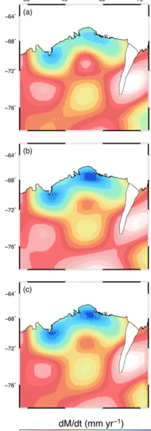
Figure 4.GRACE observations corrected for GIA uplift rates us-ing(a)the ICE-6G_C(VM5) model by Peltier et al. (2015),(b)the W12a model by Whitehouse et al. (2012), and(c)the ICE6G_ANU model by Purcell et al. (2016).
a positive anomaly between 30 and 70◦E and a substantial increase in mass between 2003 and 2009 (Fig. 4b).
The modelled trend in SMB and surface elevation due to SMB and firn compaction can now be removed from the GRACE and ICESat observations (Eqs. 11 and 12), to ob-tain dM
ice GRACE
dt and dHICESatice
dt and, subsequently,
dHGRACEice dt and dMICESatice
dt by dividing (multiplying) by the density of glacier ice. We converted the rate of change of surface elevation due to the ice dynamic signal obtained from ICESat into spheri-cal harmonics to be comparable withdH
ice GRACE
dt . By doing this, we represent the ice height information with the same
spa-tial resolution as the mass change information and impose the same potential leakage on to the altimetry observations. The estimated rate of change due to ice dynamics is shown in Fig. 5, comparing estimates obtained using two different SMB models: RACMO2.1 and RACMO2.3.
We obtained similar rates of change due to ice dy-namics by removing the modelled SMB estimates from both RACMO2 models and GIA uplift rates from GRACE and ICESat observations. When using SMB estimates from RACMO2.3, the ice dynamic estimates are significant smaller and primarily present between 30 and 60◦E with estimated rates between −0.08 and −0.13 m yr−1 obtained across the region. Using SMB estimates from RACMO2.1 yields a change due to ice dynamics of −0.08 m yr−1 and above along the entire ice sheet margin of our study re-gion, stretching across to 75◦E. Generally, when using RACMO2.3 the SMB estimates show a smaller difference between the obtained ice dynamic estimates obtained from GRACE and ICESat, improving results across the study area. However, regions remain that exhibit differences in the ob-tained ice dynamic signal of up to ±0.05 m yr−1 (Fig. 5c and f). Significant changes emerge between the rate of change due to ice dynamics obtained using the former and latter RACMO2 versions, with a root mean square error, av-eraged over the study region, of 0.019 and 0.021 m yr−1for RACMO2.3 and RACMO2.1, respectively.
In both dH
ice ICESat
dt rates a positive trend is estimated across the centre of the region. This is the result of a slightly posi-tive elevation trend that has been recorded by ICESat obser-vations in region D (Fig. 6b).
Finally, the total change in surface elevation is modelled, based on dHSMB/dt, dHfc/dt, dHGIA/dt, and dH
ice GRACE
dt (Fig. 6a). When using RACMO2.3, the result of the mod-elled rate of change of surface elevation reveals a similar pattern to the ICESat observations (Fig. 6b). In region A a negative trend of ∼ −0.1 m yr−1 between 28 and 32◦E and a positive trend of∼0.25 m yr−1at 34◦E are observed. In region B a general negative trend between −0.05 and
Figure 5.Comparison between the modelled ice dynamic rates obtained by employing SMB estimates from RACMO2.3 using(a)GRACE and (b)ICESat, and by employing SMB estimates from RACMO2.1 using(d)GRACE and(e)ICESat.(c)and (f)show the difference between ice dynamic rates obtained from GRACE minus ice dynamic rates obtained from ICESat for the employed SMB estimates obtained from RACMO2.3/ANT and RACMO2.1/ANT, respectively.
Figure 6. (a)Our modelled rate of change of surface elevation re-trieved by removing our estimated ice dynamic rates, obtained from GRACE, from the modelled trend in surface elevation (SMB minus firn compaction) using RACMO2.3, compared to (b)the ICESat observations.
the general positive trend across the region is modelled, to-gether with the positive signal near 70◦E, as well as a slight negative trend across the margin. However, the strong nega-tive trend at the Mellor Glacier is lacking, though the region does show a slight negative trend. Although the modelled trend in surface elevation suggests similar behaviour to the altimetry observations, the signal generally appears damped compared to the ICESat observations. This is likely caused by the loss of spatial resolution through the use of degree 80
spherical harmonics (the resolution of the GRACE gravity fields) to remove the ice dynamic signal.
Uncertainties are estimated for the satellite observations and models individually, and error propagation is used to ob-tain the uncerob-tainty of the modelled ice dynamic estimates and modelled surface elevation changes. The uncertainty es-timated for the modelled surface elevation trend varies be-tween near zero and∼6 cm yr−1across the interior and along large parts of the ice sheet margins, and up to 12 cm yr−1for the two locations with high SMB rates. The uncertainty of the monthly GRACE solutions are derived following the method of Wahr et al. (2006) and are∼8 mm w.e. yr−1(Fig. 7a), re-ducing towards the polar regions due to denser ground track coverage (Wahr et al., 2006). The uncertainties of the ICESat observations are below 0.05 m yr−1in the interior, where a dense network of ground-tracks exists, and between 0.15 and 0.3 m yr−1 along the ice sheet margins due to greater dis-tances between the ground tracks and steeper slopes along the margins (Hoffmann, 2016) (Fig. 7b).
Figure 7.Uncertainties estimated for(a)GRACE,(b)ICESat,(c)our monthly firn compaction model, ice dynamic rates using RACMO2.3 obtained from(d)GRACE and(e)ICESat, and the modelled surface elevation trend for(f)RACMO2.3. The greatest uncertainty comes from the ICESat measurements, with up to 30 cm yr−1at the margins; this results in greater uncertainties for the modelled ice dynamic rates obtained from the ICESat observations.
(Sutterley et al., 2014). Error sources include the parame-terisations to estimate surface snow density (Eq. 3) and the densification rate (Eq. 4), together with uncertainties within the forcing climate model RACMO2. As the firn compaction model is tuned to fit observations, it is difficult to obtain re-alistic uncertainty estimates. However, following the idea of Helsen et al. (2008), we obtain our error estimate for the firn compaction model by assessing the propagation of the major error sources that affect firn compaction rates. This was done by applying a bias to the accumulation (8 %) and tempera-ture (10 K; Reijmer et al., 2005; Maris et al., 2012), as well as to the surface snow density (±20 kg m−3; Helsen et al., 2008). The propagation of the errors is calculated to obtain the total uncertainty of the firn compaction model (Fig. 7c). Across most of the study site the uncertainty is estimated to be around±2–3 cm yr−1. However, at the two locations with the high SMB rates the uncertainty is significantly larger and is estimated to be up to 8 cm yr−1. Uncertainties for GIA models are not provided, as the models are tuned to fit ob-servations and the best-fitting ice sheet history and earth rhe-ology values (e.g. Velicogna and Wahr, 2006). However, un-certainties within our study region are small due to small up-lift rates and differences between the models of < 2 mm yr−1. Therefore, the error in the modelled GIA signals in our study region is considered negligible.
To estimate the uncertainty of the modelled ice dynamics and modelled surface elevation change, the propagation of
er-rors of the particular error source is obtained (Fig. 7d and e). Depending on the incorporated satellite mission the uncer-tainty for the modelled rate of change due to ice dynamics is up to 6 cm yr−1 (GRACE, Fig. 7d) and up to 30 cm yr−1 (ICESat, Fig. 7e), due to the larger error of the ICESat obser-vations. The uncertainty of the modelled elevation change is 0–12 cm yr−1(Fig. 7f), with the greatest error source being the firn compaction model.
6 Conclusions
Although different GIA models affect GRACE and altime-try observations in different ways, changes in GIA models have a small effect on the estimated rate of change due to ice dynamics and so are not responsible for different esti-mates using the two satellite techniques. Our data suggest that the differences are not based on errors in the ICESat ob-servations as most of the greatest differences occur in regions where ICESat uncertainties are low (Fig. 7c), in particular the large, negative difference occurring inland within the study region (significantly different from zero at the 95 % confi-dence level). Moreover, modelling the rate of change of sur-face elevation based on ice dynamic estimates obtained from GRACE observations and RACMO2.3 estimates positive and negative changes in elevation in the same regions in which ICESat detects corresponding trends, though the rates appear slightly underestimated compared to the altimetry observa-tions. Therefore, it appears that the dominant driver in the differences of the modelled rate of change due to ice dynam-ics and surface elevation trends are the changes of the SMB rates within the RACMO2 model, with RACMO2.3 provid-ing a more accurately modelled rate of change of surface el-evation. Thus, a comparison of estimated changes in ice dy-namics derived from GRACE and altimetry observations not only provides information about dynamic mass changes but may also help to identify regions where models fail to accu-rately simulate variations in SMB.
Data availability. The data and model codes used in this anal-ysis can be accessed by contacting the corresponding author, Bianca Kallenberg (bianca.kallenberg@anu.edu.au), directly. The data set containing the ICESat surface elevation changes was provided by Janosch Hoffmann. The regional climate model RACMO2/ANT was provided by Stefan Ligtenberg.
Competing interests. The authors declare that they have no conflict of interest.
Acknowledgements. This work was supported in part by an Aus-tralian Antarctic Project grant (number AAP4160).
We would like to thank Stefan Ligtenberg for providing us with the RACMO2/ANT data sets and his extensive support and constructive help to establish our own firn compaction model.
Edited by: M. van den Broeke Reviewed by: two anonymous referees
References
Allison, I., Alley, R. B., Fricker, H. A., Thomas, R. H., and Warner, R. C.: Ice sheet mass balance and sea level, Antarct. Sci., 21, 413–426, doi:10.1017/S0954102009990137, 2009.
Arthern, R. J., Vaughan, D. G., Rankin, A. M., Mulvaney, R., and Thomas, E. R.: In situ measurements of Antarctic snow com-paction compared with predictions of models, J. Geophys. Res., 115, F03011, doi:10.1029/2009JF001306, 2010.
Bruinsma, S., Lemoine, J.-M., Biancale, R., and Valès, N.: CNES/GRGS 10-day gravity field models (release 2) and their evaluation, Adv. Space Res., 45, 587–601, doi:10.1016/j.asr.2009.10.012, 2010.
Coléou, C. and Lesaffre, B.: Irreducible water saturation in snow: experimental results in a cold laboratory, Ann. Glacial., 26, 64– 68, 1998.
Cuffey, K. M. and Paterson, W. S. B.: The Physics of Glaciers, El-sevier Store, 4th Edn., Pergamon, Oxford, UK, 2010.
Ewert, H., Groh, A., and Dietrich, R.: Volume and mass changes of the Greenland ice sheet inferred from ICESat and GRACE, J. Geodynam., 59–60, 111–123, doi:10.1016/j.jog.2011.06.003, 2012.
Gunter, B., Urban, T., Riva, R., Helsen, M., Harpold, R., Poole, S., Nagel, P., Schutz, B., and Tapley, B.: A comparison of coincident GRACE and ICESat data over Antarctica, J. Geodesy, 83, 1051– 1060, doi:10.1007/s00190-009-0323-4, 2009.
Helsen, M. M., van den Broeke, M. R., van de Wal, R. S. W., van de Berg, W. J., van Meijgaard, E., Davis, C. H., Li, Y., and Goodwin, I.: Elevation Changes in Antarctica Mainly De-termined by Accumulation Variability, Science, 320, 1626–1629, doi:10.1126/science.1153894, 2008.
Herron, M. and Langway, C.: Firn Densification: An emperical model, J. Glaciol., 25, 373–385, 1980.
Hoffmann, J.: Ice height changes in East Antarctica derived from satellite laser altimetry, The Australian National University, PhD Thesis, 2016.
Kaspers, K. A., van de Wal, R. S. W., van den Broeke, M. R., Schwander, J., van Lipzig, N. P. M., and Brenninkmeijer, C. A. M.: Model calculations of the age of firn air across the Antarctic continent, Atmos. Chem. Phys., 4, 1365–1380, doi:10.5194/acp-4-1365-2004, 2004.
Kuipers Munneke, P., Ligtenberg, S. R. M., Suder, E. A., and Van Den Broeke, M. R.: A model study of the response of dry and wet firn to climate change, Ann. Glaciol., 56, 1–8, doi:10.3189/2015AoG70A994, 2015.
Lemoine, J.-M., Bruinsma, S., Gégout, P., Biancale, R., and Bour-gogne, S.: Release 3 of the GRACE gravity solutions from CNES/GRGS, Geophysical Research Abstracts, 15(EGU2013-11123), 2013.
Lenaerts, J. T. M. and van den Broeke, M. R.: Mod-elling drifting snow in Antarctica with a regional climate model: 2. Results, J. Geophys. Res.-Atmos., 117, D05109, doi:10.1029/2011JD016145, 2012.
Lenaerts, J. T. M., van den Broeke, M. R., van de Berg, W. J., van Meijgaard, E., and Kuipers Munneke, P.: A new, high-resolution surface mass balance map of Antarctica (1979–2010) based on regional atmospheric climate modelling, Geophys. Res. Lett., 39, L04501, doi:10.1029/2011GL050713, 2012.
Maris, M. N. A., de Boer, B., and Oerlemans, J.: A climate model intercomparison for the Antarctic region: present and past, Clim. Past, 8, 803–814, doi:10.5194/cp-8-803-2012, 2012.
Mouginot J., Scheuchl, B., and Rignot, E.: Mapping of Ice Mo-tion in Antarctica Using Synthetic-Aperture Radar Data, Remote Sensing, 4, 2753–2767, doi:10.3390/rs4092753, 2012.
Pagiatakis, S. D.: The response of a realistic earth to ocean tide loading, Geophys. J. Int., 103, 541–560, 1990.
Peltier, W. R., Argus, D. F., and Drummond, R.: Space geodesy constrains ice age terminal deglaciation: The global ICE-6G_C (VM5a) model, J. Geophys. Res.-Sol. Ea., 120, 450–487, doi:10.1002/2014JB011176, 2015.
Pritchard, H. D., Arthern, R. J., Vaughan, D. G., and Edwards, L. A.: Extensive dynamic thinning on the margins of the Greenland and Antarctic ice sheets, Nature, 461, 971–975, doi:10.1038/nature08471, 2009.
Purcell, A., Dehecq, A., Tregoning, P., Potter, E.-K., McClusky, S. C., and Lambeck, K.: Relationship between glacial isostatic ad-justment and gravity perturbations observed by GRACE, Geo-phys. Res. Lett., 38, L18305, doi:10.1029/2011GL048624, 2011. Purcell, A., Tregoning, P., and Dehecq, A.: An assessment of the ICE6G_C(VM5a) glacial isostatic adjustment model, J. Geo-phys. Res.-Sol. Ea., 121, 3939–3950, 2016.
Reijmer, C. H., van Meijgaard, E., and van den Broeke, M. R.: Eval-uation of temperature and wind over Antarctica in a Regional Atmospheric Climate Model using 1 year of automatic weather station data and upper air observations, J. Geophys. Res., 110, D04103, doi:10.1029/2004JD005234, 2005.
Rémy, F. and Frezzotti, M.: Antarctica ice sheet mass balance, C. R. Geosci., 338, 1084–1097, doi:10.1016/j.crte.2006.05.009, 2006. Rignot, E.: Changes in ice dynamics and mass balance of the Antarctic ice sheet, Philos. T. R. Soc. A, 364, 1637–1655, doi:10.1098/rsta.2006.1793, 2006.
Rignot, E. and Thomas, R. H.: Mass Balance of Polar Ice Sheets, Science, 297, 1502–1506, doi:10.1126/science.1073888, 2002. Rignot, E., Bamber, J. L., van den Broeke, M. R., Davis, C., Li, Y.,
van de Berg, W. J., and van Meijgaard, E.: Recent Antarctic ice mass loss from radar interferometry and regional climate mod-elling, Nat. Geosci., 1, 106–110, doi:10.1038/ngeo102, 2008. Rignot, E., Mouginot, J., and Scheuchl, B.: MEaSUREs
InSAR-Based Antarctica Velocity Map, Boulder, Colorado USA: NASA EOSDIS Distributed Active Archive Center at NSIDC, available at: http://nsidc.org/data/nsidc-0484.html (last access: 3 April 2015), 2011.
Rignot, E., Jacobs, S., Mouginot, J., and Scheuchl, B.: Ice-Shelf Melting Around Antarctica, Science, 341, 266–270, doi:10.1126/science.1235798, 2013.
Sasgen, I., Konrad, H., Ivins, E. R., Van den Broeke, M. R., Bamber, J. L., Martinec, Z., and Klemann, V.: Antarctic ice-mass balance 2003 to 2012: regional reanalysis of GRACE satellite gravimetry measurements with improved estimate of glacial-isostatic adjust-ment based on GPS uplift rates, The Cryosphere, 7, 1499–1512, doi:10.5194/tc-7-1499-2013, 2013.
Shepherd, A., Ivins, E. R., Geruo, A., Barletta, V. R., Bentley, M. J., Bettadpur, S., Briggs, K. H., Bromwich, D. H., Fors-berg, R., Galin, N., Horwath, M., Jacobs, S., Joughin, I., King, M. A., Lenaerts, J. T. M., Li, J., Ligtenberg, S. R. M., Luck-man, A., Luthcke, S. B., McMillan, M., Meister, R., Milne, G., Mouginot, J., Muir, A., Nicolas, J. P., Paden, J., Payne, A. J., Pritchard, H., Rignot, E., Rott, H., Sørensen, L. S., Scambos, T. A., Scheuchl, B., Schrama, E. J. O., Smith, B., Sundal, A. V., van Angelen, J. H., van de Berg, W. J., van den Broeke, M. R., Vaughan, D. G., Velicogna, I., Wahr, J., Whitehouse, P. L., Wing-ham, D. J., Yi, D., Young, D., and Zwally, H. J.: A Reconciled Estimate of Ice-Sheet Mass Balance, Science, 338, 1183–1189, doi:10.1126/science.1228102, 2012.
Slobbe, D. C., Lindenbergh, R. C., and Ditmar, P.: Estimation of volume change rates of Greenland’s ice sheet from ICESat data using overlapping footprints, Remote Sens. Environ., 112, 4204– 4213, doi:10.1016/j.rse.2008.07.004, 2008.
Sørensen, L. S., Simonsen, S. B., Nielsen, K., Lucas-Picher, P., Spada, G., Adalgeirsdottir, G., Forsberg, R., and Hvidberg, C. S.: Mass balance of the Greenland ice sheet (2003–2008) from ICE-Sat data – the impact of interpolation, sampling and firn density, The Cryosphere, 5, 173–186, doi:10.5194/tc-5-173-2011, 2011. Sutterley, T. C., Velicogna, I., Csatho, B., van den Broeke, M.,
Rezvan-Behbahani, S., and Babonis, G.: Evaluating Greenland glacial isostatic adjustment corrections using GRACE, altimetry and surface mass balance data, Environ. Res. Lett., 9, 014004, doi:10.1088/1748-9326/9/1/014004, 2014.
Van Wessem, J. M., Reijmer, C. H., Morlighem, M., Mouginot, J., Rignot, E., Medley, B., Joughin, I., Wouters, B., Depoorter, M. A., Bamber, J. L., Lenaerts, J. T. M., Van De Berg, W. J., Van Den Broeke, M. R., and Van Meijgaard, E.: Improved representation of East Antarctic surface mass balance in a re-gional atmospheric climate model, J. Glaciol., 60, 761–770, doi:10.3189/2014JoG14J051, 2014.
Velicogna, I. and Wahr, J.: Measurements of Time-Variable Grav-ity Show Mass Loss in Antarctica, Science, 311, 1754–1756, doi:10.1126/science.1123785, 2006.
Wahr, J., Molenaar, M., and Bryan, F.: Time variability of the Earth’s gravity field: Hydrological and oceanic effects and their possible detection using GRACE, J. Geophys. Res., 103, 30205– 30229, 1998.
Wahr, J., Swenson, S., and Velicogna, I.: Accuracy of GRACE mass estimates, Geophys. Res. Lett., 33, L06401, doi:10.1029/2005GL025305, 2006.