Simulation methods and economic analysis

Simulation Methods and Economic

Analysis

Hamish W. Low

Septem ber 1998

ProQ uest Number: U 643012

All rights reserved

INFORMATION TO ALL U SE R S

The quality of this reproduction is d ep en d en t upon the quality of the copy subm itted. In the unlikely even t that the author did not sen d a com plete manuscript

and there are m issing p a g e s, th e se will be noted. Also, if material had to be rem oved, a note will indicate the deletion.

uest.

ProQ uest U 643012

Published by ProQ uest LLC(2015). Copyright of the Dissertation is held by the Author. All rights reserved.

This work is protected against unauthorized copying under Title 17, United S ta tes C ode. Microform Edition © ProQ uest LLC.

ProQ uest LLC

789 East E isenhow er Parkway P.O. Box 1346

C on ten ts

A bstract 6

A cknow ledgem ents 8

D eclaration 9

1 Introdu ction 10

2 N um erical M ethods for Solving F in ite H orizon D ynam ic

M odels 15

2.1 Introduction... 15

2.2 Numerical I n te g r a tio n ... 20

2.3 Approximation M e th o d s ... 23

2.3.1 D iscretisation... 23

2.3.2 Interpolation and A pproxim ation... 26

2.4 Inequality C o n s tra in ts ... 40

2.5 Conclusion ... 43

3 Self-Insurance, Life-Cycle Labour Supply and Savings B e­ haviour 45 3.1 Introduction... 45

3.2 L ite r a tu r e ... 49

3.4 Solution M e t h o d ... 57

3.5 Life-Cycle B eh av io u r... 71

3.5.1 Life-Cycle P r o f ile s ... 72

3.5.2 Comparing Models with Exogenous and Endogenous Labour S u p p ly ... 81

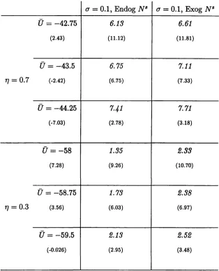
3.6 Welfare Cost of U n c ertain ty ... 93

3.7 Conclusion ... 96

4 Particip ation A cross th e Life-cycle 98 4.1 Introduction... 98

4.2 Secondary Earner P a rtic ip a tio n ... 103

4.2.1 Solution M e t h o d ... 105

4.2.2 Simulated Life-Cycle P r o f ile s ...106

4.3 Social S e c u r i t y ...116

4.3.1 Solution M e th o d ... 118

4.3.2 Simulated Life-cycle Profiles... 123

4.4 Conclusion ... 133

5 Long R un Equilibria: E xpected W aiting T im es w ith N o isy Selection and Local Interaction 135 5.1 Introduction... 135

5.2 Selection P r o c e s s ...142

5.3 Simulated Waiting T i m e s ... 149

5.4 Simulated D is trib u tio n s ...158

5.5 Robustness of the Selection R e s u l t ... 162

L ist o f Tables

3.1 Average Consumption Growth, Varying v ... 84

3.2 Expected Cost of achieving Expected Utility, Ü ... 95

4.1 Average Household Consumption G r o w t h ... I l l 4.2 Tax Rates to Pay for Social S e c u rity ... 125

5.1 Simulated Waiting T i m e s ...152

5.2 Time for First Island C o n v erg en ce... 155

5.3 Average Waiting Times, Islands on a C i r c l e ... 157

5.4 Probability of a Shift to Risk-Dominance ... 161

5.5 CoeflScients of Variation of Waiting Times ... 161

5.6 Probability Mass R a t i o s ...165

L ist o f F igures

2.1 Lagrange Interpolation ... 29

3.1 Solution for Leisure ... 68

3.2 Solution for Total W ithin Period Spending ... 69

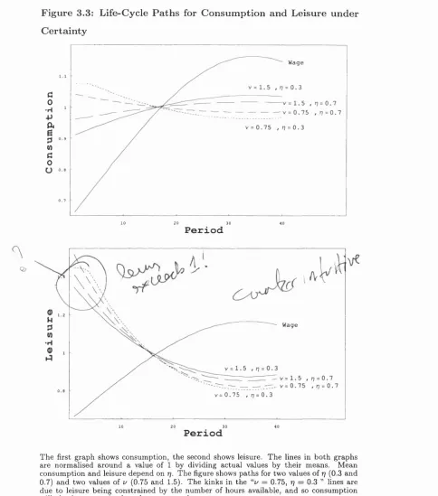
3.3 Life-Cycle Paths for Consumption and Leisure under Cer­ tainty 75

3.4 Life-Cycle Paths for C o n s u m p tio n ... 76

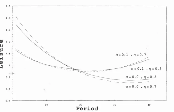
3.5 Life-Cycle Paths for Leisure ... 78

3.6 Asset Accumulation across the L ife -C y c le ... 80

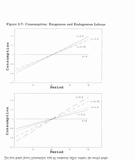
3.7 Consumption: Exogenous and Endogenous L a b o u r ... 83

3.8 Consumption: Varying rj and i / ... 85

3.9 Leisure Smoothing: Varying rj and i / ... 87

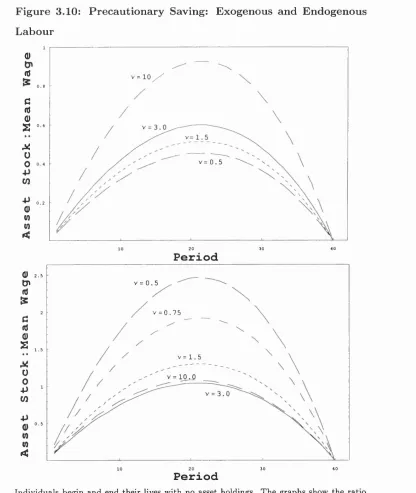
3.10 Precautionary Saving: Exogenous and Endogenous Labour . 89 3.11 Precautionary Saving: Varying rj and ... 91

4.1 Household Asset A ccu m u latio n ... 109

4.2 Individual and Household Leisure S m o o th in g ... 114

4.3 Non-Participation across the Life-Cycle ...115

4.4 Reservation Asset Levels across the Life-cycle... 126

4.5 Non-Participation with Unemployment B e n e f i t ... 129

4.6 Asset Accumulation with Unemployment B e n e f it... 132

A b stra ct

There are two parts to this thesis: the first analyses the joint determination of saving and labour supply under uncertainty, using numerical dynamic programming to model life-cycle behaviour. The second uses simulation to analyse the problem of equilibrium selection when individuals are myopic and interaction between individuals is predominantly local. The value of using simulation methods is th at this enables the analysis of more complex and realistic models than is analytically feasible.

simulations show how labour supply and participation choices change across the life-cycle and how these choices interact with the savings decision.

A cknow ledgm ents

Particular thanks are due to Costas Meghir and to Orazio Attanasio, Ken Binmore and Richard Blundell. I am also grateful for helpful comments to Kazunori Araki, James Banks, Nick Bloom, Tilman Borgers, Ian Crawford, Amanda Gosling, Ken Judd, Ellen McGrattan, Greg Pollock, Ian Preston, Larry Samuelson, Sarah Tanner, Harald Uhlig, Joachim Winter and seminar participants at IPS, UCL, Tilburg, Cambridge and the 1998 TMR conference on savings at Deidesheim. Chapter 5 is joint work with Kazunori Araki. Finally, I am especially grateful to Amanda Low for many helpful discussions and much support.

D eclaration

No part of this thesis has previously been presented to any University for any degree.

C hapter 1

In trod u ction

There are two parts to this thesis: the first combines dynamic models of saving under uncertainty with models of labour supply. This is to address three main questions, not currently addressed in the literature: what are the implications for consumption smoothing and precautionary saving of allowing individuals to vary their labour supply; what are the effects of social security on asset accumulation and participation across the life-cycle; and finally, in a household setting, at what stages in their lifetimes will secondary earners participate in the labour force and how does this affect household saving?

The second part of this thesis addresses the problem of equilibrium se­ lection when individuals are myopic. One of the key issues here is how long it takes for a particular equilibrium to be reached. The aim of this part of the thesis is to show the impact on this length of time both of the type of in­ teraction between individuals and of the extent of mistakes th at individuals make in updating their strategies.

values. However, estimation of parameters in the first part of the thesis would require the numerical solution of the stochastic dynamic programming problem as a step within any estimation routine.

L ife-C ycle Saving and Labour Supply under U ncertain ty

Chapter 2 discusses the numerical methods used in this part of the thesis for solving finite horizon dynamic models. The purpose of this is to justify the methodology and to show when alternative methods would be appropriate.

Models of optimal saving under uncertainty (e.g. Deaton, 1992) show th a t individuals save today to provide extra resources for periods when wages are lower than expected. This precautionary saving is provided by sacrific­ ing consumption because labour supply is assumed to be fixed. Chapter 3 relaxes this assumption and so precautionary accumulation occurs partly through increased labour supply when young. Further, the flexibility in labour supply means individuals can react to negative shocks to wages by increasing leisure. This ability to adjust labour supply means uncertainty is less costly to individuals, and consumption paths will be smoother. The effect on precautionary saving is ambiguous, however: the benefit of pre­ cautionary balances is lower when labour is flexible because of the ability to react to low wage realisations, but the cost of providing balances is also lower because saving occurs through increased labour as well as decreased consumption.

Modelling household rather than individual choice, means there are two sources of income and thus some insurance against uncertainty. However, primary earner labour supply is assumed to be fixed and this reduces the ability of households to react to uncertainty by varying leisure. The net effect depends on the correlation between the secondary and primary earner wages. As this becomes increasingly negative, secondary earner labour offers increasingly effective insurance. This means th at secondary earners either work a large number of hours or not at all, depending on the income of their partners. In this model, participation falls with age because the revelation of uncertainty reduces the need to work for precautionary reasons.

Social security is introduced in the form of a benefit th at is paid if the in­ dividual is not working. Social security thus provides insurance against the uncertainty of future wages and this reduces asset accumulation. However, individuals know they might have periods when they do not work at all, and this encourages asset accumulation in order to smooth consumption. The level of participation decreases with the generosity of benefits, but partici­ pation is greatest at the start and at the end of the life-cycle. This increase in participation with age is in contrast to the earlier result for secondary earners, and is also in contrast to the results of Eckstein and Wolpin (1989). Non-participation here is driven by the intertemporal substitution of labour, and as the number of remaining periods of life falls, such substitution possi­ bilities are limited; whereas in Eckstein and Wolpin participation falls with age because there are fewer remaining periods for experience to impact on the expected wage.

W aiting T im es for Equilibrium Selection

are many tests in the literature of whether individual behaviour conforms to the solution of particular dynamic problems, (surveyed in Rust, 1994), but in cases where behaviour does not conform to the solution of a particular opti­ misation problem, there are two broad strategies: first, to treat the failure as a failure of the particular model and then to make the optimisation problem more sophisticated; or second, to treat the failure as a failure of behaviour to conform to optimisation and to model methods of imperfect optimisa­ tion. P art of the motivation for the first part of this thesis, in chapters 3 and 4, was to develop a more sophisticated model of individual choice which may explain apparent failures in observed consumer behaviour to conform to the optimal paths described by models with an exogenous labour supply (as discussed by Deaton, 1992). By contrast, part of the motivation for the second part of this thesis (chapter 5) is to model how observed behaviour would evolve if individuals were behaving as imperfect optimisers.

The model analysed in chapter 5 is not a single-person decision problem of the type modelled in chapters 3 and 4,^ but a strategic problem where the best strategy of each player depends on the types of the other players. There has been much research into analysing which strategies will become more common in such a setting when individuals follow rules of thumb rather than solve the particular optimisation problem. In particular, there has been much research into what sort of equilibrium will be selected when individ­ uals are not fully rational (for example, Kandori et al, 1993; and Young, 1993). One criticism of this approach (discussed by Ellison (1993) and oth­ ers) is th a t the expected waiting times to reach the selected equilibrium are sometimes fantastically large, particularly as population size increases. This reduces the value of such selection results for applied settings. Chapter 5

^For single-decision problems, Lettau and Uhlig (1995) discuss learning processes that

lead to non-optimal behaviour. However, in the non-strategic framework most learning

processes appear to lead to optim al decision making, if the environment is sufHciently

has two main aims, therefore: first, to discuss when expected waiting times will be lower; second, to question the focus solely on expected waiting times; and third, to discuss when such models are relevant in an economic context. These questions are addressed by combining a model in which interaction is predominantly between neighbours with a model with significant noise in the payoffs to different strategies. Simulation is used to address these ques­ tions because the combination of the form of interaction and the uncertainty in the payoffs means analytic solutions are intractable.

C hap ter 2

N u m erical M eth o d s for

S olvin g F in ite H orizon

D yn am ic M od els

2.1

In trod u ction

This chapter surveys the alternative methods of solving finite horizon dy­ namic models, and discusses the implementation of such methods. The aim of this is to justify the methodology used in subsequent chapters and to discuss when alternative methodologies would be appropriate.^

A wide range of dynamic models can be solved by dynamic programming and hence they can be solved through a recursive set of functional equations. Each of these functional equations has the general form:

g { y { x ) , x ) = {) (2.1) where g (•, •) is known, and x is the vector of state variables. The function

y{x) is the unknown policy function th at solves (2.1). The difficulty with

^This description draws on Judd (1998), McGrattan (1996), Rust (1996), Christiano

solving this equation arises if the state variables are continuous and so solv­ ing (2.1) is analogous to solving a continuum of equations for a continuum of unknowns (one unknown for each element of the state space).^ The following standard example highlights the issues involved in solving such functional equations.

Exam ple: O ptim al Saving

This example is the simple partial equilibrium, optimal saving problem fac­ ing consumers:

T

max Et (cg) (2.2)

s= t

subject to

and

As+i = (1 + r) [As + - Cs] (2.3)

■^«+1 > —A (2.4)

where T is the horizon length which is assumed to be finite, although some comparisons are made with the infinite horizon case. /3 is the discount factor, r the deterministic interest rate. At the asset stock at the start of period t,

and Wt is stochastic income received in t which follows some known Markov process, which can be discrete or continuous. The constraint (2.4) is the constraint on borrowing,^ which must be less than A . The state of the world in each period is given by {^4*, wt] , which in special cases reduces to a single state variable, cash-in-hand.

* There can also be a problem if the state space is discrete when there are many possible

states, but this chapter focuses on problems with a continuous state space and continuous

controls.

^Strictly, the constraint is on the amount of borrowing in t, rather than the asset

stock at the start of t -|- 1. However, there is a trivial equivalence if the interest rate is

deterministic.. If the interest rate is stochastic, maximum borrowing is determined by the

The problem can be solved by setting up the Lagrangian or by using Bellman’s equation. The first order conditions of the Lagrangian reduce to

p

a c . . . J ^ "

(2.5)

Af+1 > —A (2.6)

If the borrowing constraint never binds, the problem reduces to solving (2.5)

as an equality. When T is finite, the problem is non-stationary and the solution proceeds by backward induction, solving for ct (At,it;*), given the solution to ct+i (At+i,it;t4. i ) . When T = oo and the problem is stationary, the solution is for c (A, w) .

The problem can also be written recursively using Bellman’s equation,

Vt (At,wt) = max {u (c*) + /3Et [Vt+i (A*+i, wt+i)]} (2.7)

ct

This also gives rise to the first order conditions (2.5) and (2.6).

Equation (2.7) highlights the difference between the finite and infinite horizon models. When T is finite, equation (2.7) explicitly defines the maximum value function, V* { A ^ w t ), th at the individual can achieve when Ct (At, W t ) is chosen optimally, given the value function for the following pe­ riod. This solution Vt{AtyWt) is then used in the solution to

Vt-i {At-iyWt-i) . When T is infinite, equation (2.7) only implicitly defines the value function, because the same function is used for period t and for

function. This new value function is the next guess at the stationary solu­ tion for the infinite horizon model, but is the value function specific to T — 1 for the finite horizon model. Iteration or backward induction continues until V « r [V] or t = 1, respectively for the infinite and finite horizon cases.^

The most time consuming element of backward induction, and indeed value function iteration, is the solution of the maximisation problem on the right hand side of (2.7). The function is maximised by solving the first order conditions (2.5) and (2.6) for the policy function, ct{At,wt). This chapter is a discussion of methods of solving such functional equations.

The example highfights the main issues involved. The solution to (2.5) is a function which maps from the state space {At, wt} into consumption, ct. It is not possible to solve this functional equation analytically when marginal utility is non-linear, and it is not possible to solve numerically for consump­ tion at all possible states of the world, given a constraint on computing time. This means it is necessary to use some numerical approximation to the solution. The first issue is th at the expectations operator in (2.5) in­ volves integration with no tractable analytic solution. The integral must therefore also be approximated numerically, using either Monte-Carlo or Gaussian Quadrature. The best method of approximation depends crucially on the number of dimensions of the state space th a t the integration is over. Gaussian quadrature tends to be faster for a given degree of accuracy when the dimension is low (e.g. less than 3), but quickly becomes subject to the “curse of dimensionality” as the dimension increases. This issue is analysed first in this chapter in order to introduce the ideas of orthogonal polynomials and approximation. The second issue is how to approximate the function

^For infinite horizon models, there is much debate in the literature (e.g. Rust, 1996;

Judd, 1998) about whether the solution method should iterate over the value function,

or over the policy function giving the optimal action, or use some other acceleration

technique. This debate is not relevant to finite horizon models where it is always necessary

giving the solution across the whole state space: this can either be through fitting an interpolating function to specific points in the state space; or it can be through approximating the solution directly by some function which is parameterised by a vector of values. Both methods either explicitly or implicitly involve discretising the state space, and this raises the issue of the optimal discretisation. This issue is clearly related to the method of numerical integration. The third issue is how to incorporate the inequality constraint: this can be done either by approximating the Lagrange multiplier function directly or incorporating the inequality through a penalty function in utility. Introducing inequality constraints changes the desirability of dif­ ferent approximation methods. Underlying each of these issues is the desire to minimise the error involved in using a numerical solution rather than an analytic solution. Before discussing these issues in detail, however, it is necessary to discuss when the use of such numerical methods is unnecessary.

The reason why it is necessary to use numerical methods to solve equa­ tion (2.5) is th at n' (•) is non-linear (or, more generally, g{y{x) ,x) is non­ linear in y{x)). If g{y{x) ,x) were linear in y (x ) (in particular, if the ob­ jective of the underlying problem is quadratic and the constraints linear),

which are linear-quadratic particularly easy to solve, but often uninteresting in their implications.^ Further, using a linear-quadratic approximation to more general models may be very inaccurate, and in particular, making such an approximation involves ruling out a substantive role for uncertainty.

2.2

N um erical Integration

The idea underlying numerical integration is to approximate the true inte­ grand by some polynomial or function th at is easy to integrate, and then to integrate th at polynomial. There are three broad approaches to this: the first approach is to discretise the domain of the integrand into subdo­ mains and then, within each subdomain, to fit a low order polynomial to the solution at the selected points of the domain, i.e. giving a piecewise polyno­ mial approximation to the true integrand. For example, the domain can be discretised uniformly and linear functions fitted between the values of the integrand at the discrete points. This piecewise polynomial approximation is then integrated. This is known as Newton-Cotes integration, and for a given set of discretised points, chooses the weights to put on the value of the integrand at each particular point. Thus,

N

h { x ) d x ^ ^ 2 ^ ( ^ n ) W n ( 2 . 8 )

n=l

where N is the number of discrete points.

The second method, called Gaussian Quadrature, is to approximate the integrand using one polynomial of degree N across the whole domain, where the integrand is evaluated at N points. Both the N abscissae and the cor­ responding weights are chosen optimally and the approximation is exact for any polynomial of degree (2N — 1) or less. The choice of weights and points

/

® However, Hansen and Sargent (1998) use a linear-quadratic framework throughout

their book because the ease of solution means much more complex problems can be

/

depends on the underlying form of the integrand. If integration is over a random variable which has a density / (x), the integral can be approximated as follows

(2.9) where the are the appropriate abscissae, and are the corresponding weights to be used. W (xn) is the weighting function underlying the choice of abscissae. The function h (x) is called the kernel of the integration process.

The discrete approximation is the integral of a polynomial which approx­ imates the true integrand, and so the closer the fitting polynomial is to the true integrand, the better the approximation. The discrete approximation will therefore be better when W (x) = f ( x ) . This observation also suggests the optimal abscissae to use in the discretisation: the abscissae should be chosen to make integration of the approximating polynomial as accurate as possible. Given the form of W (x) is suggested by / (x) , the abscissae are chosen as the roots of the polynomial (^) where pjv (x) is chosen so th a t

PN (x) Pj (^) W (x) dx = 0, N (2.10)

I

In other words, (z) is orthogonal to pj (x) for the weighting function

W (x) in the interval [o, b] where pj (x) is a polynomial of different order to

PN (x) but of the same family.®

For example, if expectations are over a random variable which is nor­ mally distributed, (/x, , then the integral can be well approximated by Gaussian Hermite quadrature. The density of the normal is given by / (x) =

exp ^ (x — , and the underlying weighting function of Gauss

®A function f ( x ) is said to be orthogonal to g ( x ) in the interval [o,6] for a given

weighting function W (z) if

rb

/:

The left hand side of this expression gives the scalar product of / (z) and g ( z ) , { f \ g ) .

Hermite is W (x) = exp ( x ^ ) . By transforming the random variable into a standard normal, the approximation will be “close” . In other words, the integral can be approximated as follows

vk J1 ^

^

5

(^)

(2.11) where the are the abscissae given by the roots of the N degree Hermite polynomial, and a;„ are the corresponding weights to be used. Similarly, if the random variable, y, is log-normally distributed, Gaussian Hermite quadrature can be used by using the change of variable, x = \n y .

For low dimensional problems, Gaussian quadrature can be very accu­ rate and fast, but it is subject to the “curse of dimensionality” in multi­ dimensions because the number of node points increases by a factor of

N with each additional state variable. This leads to the third method, Monte-Carlo integration. The procedure for the basic Monte-Carlo strategy is straightforward: N draws are made from the distribution / (x) and the unknown integral is then approximated by.

2.3

A p p roxim ation M eth od s

There are two conceptually distinct approaches to approximating the solu­ tion to equation (2.1). The first method, known as discrete approximation, solves a discrete problem which is an approximation to the continuous prob­ lem. This gives the solution to the optimal policy at a discrete set of points. The second method is to approximate the policy function itself. In practice, this involves either explicitly or implicitly using the values from a discrete problem as d ata in a least squares or other approximation method. There is clearly a large overlap between the two approaches, and this section begins with a discussion of optimal methods of discretisation. The section then analyses the way the solution at discrete points can be used to approximate the solution function. There is a distinction here between methods which solve for the discrete values independently of the approximation method and weighted residual methods which only implicitly solve the solution at a discrete set of points.^

2 .3 .1 D is c r e tis a tio n

The first method discretises the state space into a grid of N points and then solves equation (2.1) or (2.5) at each discrete node on the grid. Solving the equation becomes easy when each node is considered separately because the equation is being solved for a particular value rather than a function. The idea is th at the solution is evaluated at all points th a t will be needed in solving equation (2.7) for the previous period, and all points th at will be needed in subsequent simulations. This means th at from any point in the (continuous) state space in t, the system can only move to a finite number of points in t-bl. Thus, the density / {xt+i \xt) is approximated by / {xk,t+i k t ) where Xk,t+i is the point in the state space th at approximates any point in a given subset of the state space in f + 1, labelled k. If it is also assumed

th at xt can only take a finite number of values, the conditional probability becomes f {xk^t+i k i.t) » where Xj^t is defined analogously to Xk^t+i-> and the continuous Markov process is approximated by a discrete Markov process.

Discretising the exogenous state variable means th at the integral for the expectation operator across the continuous state space in 1 4-1 in equation (2.7) or (2.5) is replaced by a summation across a finite number of points, indexed n 6 . ,iV}. Tauchen and Hussey (1991) suggest th at the dis­ crete points in the state space should be chosen according to the appropriate method for numerical integration. This normally means using the abscissae for the appropriate Gaussian rule (for example, using the N abscissae of N

degree Gaussian Hermite integration when the exogenous state variable is normally distributed).

There is a complication to this which arises because the probability in the discrete approximation to the integral of equation (2.9) is unconditional, whereas persistence in shocks means the relevant probability for the expec­ tations operator is conditional. Therefore, the expectations integral is of the form / h (xt+i) f (xt+i \xt)dxt+i, and so has to be transformed into the form (2.9) as follows:

/

/ {xt+\ \ x t - ^i). Hence,

N

[ h{xt+i)f{xt+i \xt)(tct+i w ^ h (xk,t+i) ( 7 / \ I

V

L / ( ^ M+ 1 F i . t ~

J

(2.14) The term in {•} can be converted into the probability of moving from state

j to state k by normalising to make the terms sum to 1. In other words,

P

\H t

i,

Each value, xj^t is a discrete point in the state space of period t for which the integral for t + 1 must be evaluated. These points are chosen to be the abscissae of the integration th at will be carried out in t — 1. When the stochastic process is stationary, this means the abscissae will be constant across time.

Thus, the continuous Markov process has been replaced by a discrete process with a transition matrix and the grid across xt has been defined for all t. The choice of abscissae and weights for this transformation do not have to correspond to a particular Gaussian rule, but the appropriate Gauss rule provides the closest discrete approximation to the continuous process.

For the endogenous state variable (e.g. the asset stock. At), the choice of grid points is less clear cut. As discussed below, the optimal choice will depend on any method of interpolation or approximation th a t may be used, but the aim of grid point selection is to put more points where the derivative of the function is changing. This is often where the asset stock is close to zero, prompting the use of a uniform grid across the log of the asset stock (if A = 0). In any case, as the mesh of the grid becomes increasingly fine, the solution becomes increasingly accurate.

can break the curse of dimensionality if the set of possible actions is finite. This is because randomisation can break the curse of dimensionality involved in the evaluation of the conditional expectation. The restriction to discrete action sets is necessary because solving the general multivariate optimisa­ tion problem associated with a continuous action set is itself subject to the curse of dimensionality. Again, the issue of the curse of dimensionality is particularly important when these methods are used as subroutines in an estimation procedure.

2 .3 .2 I n te r p o la tio n Eind A p p r o x im a tio n

When the solution vector to the discrete problem is used as data in an in­ terpolating routine, the underlying idea is to approximate the actual policy

function rather than just to provide the optimal action at a set of points. This is known as smooth approximation. There are two classes of smooth approximation methods: the first takes the data from the discrete problem as given and fits an interpolating function to the data; the second class of methods, known as projection methods, explicitly tries to fit a known func­ tion to the actual policy function. In practice, the difference is small because the grid nodes will be chosen optimally whichever method, and because the projection method works by approximately fitting a known function to the values of the actual policy function at a number of discrete points. The different approaches to smooth approximation are discussed below, but first it is necessary to compare smooth approximation methods with the discrete method described above.

relatively good approximations within a reasonable time because, relative to discrete approximation, fewer node points are needed to obtain a given accuracy, if the true solution is sufficiently smooth. Second, the stability or sensitivity of the solution is important. In other words, is the approximated policy function robust to the addition of extra nodes, or the removal of nodes from the state space? This is a problem especially when using global approximation methods with few degrees of freedom. The intuitive reason for using smooth approximation methods is th a t they exploit the imposed smoothness of the solution in solving for the node values and this makes the method more time efficient. The key problem with these methods is that they need the underlying function to have a degree of smoothness.

The vector describing the solution at a set of discrete points can be used as the data in fitting an interpolating function or carrying out a least squares regression to give an approximation to the policy function at points th at are not nodes on the grid.® Least squares regression chooses a function parame- terised by M values to fit a set of N data points, where M < N. This means th at the function will not fit the N values exactly. Interpolation chooses a function which fits all N points exactly. In other words, a function para- meterised by M values, where M = N (i.e. leaving no degrees of freedom). This interpolating function may be a spline or any polynomial (up to the jVth degree, where N is the number of nodes).

Judd (1998) surveys the alternative ways of approximating a function when the solution values, j/n, are known at a set of abscissae, Xn. If we first consider methods th at leave no degrees of freedom, the main distinction to draw is between local and global approximation methods. Local methods include Taylor and Padé approximation, but more generally, local methods determine the approximate value of y (x) by the values of the solution at points in the state space close to x. This includes all piecewise polynomial

interpolation schemes. For example, a cubic spline is a piecewise polyno­ mial where the individual polynomials are smooth and, further, the different polynomials connect in a smooth way. This is a local approximation method because the approximated value of y (x) depends only on values of y (x) and

y' (x) at neighbouring nodes. Because these methods are local, they pro­ vide no indication of the optimal choice of grid points, but they do have the strength th a t the behaviour of the solution at the edges of the grid will not affect the interior solution. Finite element methods are another type of piecewise polynomial approximation. These are methods which split the state space into subdomains and then fit low order polynomials to the solu­ tion within each subdomain. The global approximation to y (x) is obtained by piecing together these local approximations. As discussed in section 2.4 below, local approximation methods and finite element methods in particu­ lar can be very useful when there are kinks in the policy function.

The most basic global method of approximation given N data points

(xn,yn) is Lagrange interpolation. This involves approximating y (x) by the degree N — 1 polynomial,

N

= (^) (2.16)

n = l

infor-mation. One classic example of Lagrange interpolation producing a poor approximation to the underlying theory is where f (x) = (l 4- and interpolation is between equally spaced nodes on [—5,5], as shown in figure 2.1. When N = 50, the approximation becomes even worse, with values of / (x) ranging between 5 and -100, and so increasing N does not improve the approximation.

F ig u re 2.1: L agrange In te rp o la tio n

2 2 •2 2

The figure shows Lagrange interpolation of f (x) = \ j y j(1 4- x^) with the true solution given by the solid lines. The left-hand graph uses 10 interpolation nodes, and the right-hand graph 11 nodes.

The point about this failure is that it arises partly because of the choice of uniform spacing of grid points. A different choice of grid points would produce a better approximation. This motivates the issue of optimal grid choice. For example, if the nodes were the zeros of a Chebyshev polynomial, as discussed below, the approximation becomes much more reasonable, and is very similar to the Chebyshev approximation. However, the underlying problem in the above example is that, although the interpolation fits the true function exactly at the nodes, there is no guarantee that the approximation will be good elsewhere. In particular, it is possible that the approximation will be good for almost all x and then very poor for some x. Thus much of what follows is a discussion of methods which can bound the maximum error.

P rojection M ethods

Equation (2.16) is one particular method of linear polynomial approximation to y (x) In general, the approximation is assumed to be a finite linear com­ bination of known functions, called basis functions, which are usually some simple function (e.g. spline, piecewise linear or Chebyshev polynomials):

M

y<p (^) = (a:) (2.17)

m = l

where M < N. The basis functions, Çîm {x) for m e {1,..., M } , are a family of polynomials, each of diflferent degree, m. The solution is parameterised by the values and the idea is th at the are chosen to make (x) close to y ( x ). One simple choice of basis function is the polynomial Clm (x) =

x'^. However, this performs very badly because the terms of (2.17) become increasingly collinear as m increases and so estimates of y using (2.17) are likely to be poor.

Projection methods are a particular class of methods for choosing which aim to make the residual of equation (2.1) “small” . This “smallness” is weaker than requiring the equation to be zero across the whole state space: the requirement is that the weighted residual of the equation be zero. This requirement can be expressed as:

{ R{ x ; y ^ ) ,(l>(x)) =

J

^Methods of nonlinear polynomial approximation include, for example, neural net­

works, and are not surveyed here.

These m ethods are also referred to as “minimum weighted residual m ethods”. How­

ever, Rust (1996) uses the term “minimum weighted residual m ethods” to refer to projec­

tion m ethods where the projection is determined by the first order condition of the general

The advantage of projection methods is that, if the policy function is itself smooth, then it can be parameterised by a number of values, M, which is less than the number of distinct nodes that would be needed for a good discrete approximation. W ith finite horizon models, the advantage of this is that the particular value of the value function or policy function at ar­ bitrary points in the state space can be found quickly and with little stor­ age requirements. This speeds up each iteration in the backward induction process. W ith infinite horizon models, projection methods can be used in a similar way to speed up each iteration of the contraction, but the methods can also be used to solve the implicit function th at defines the value function directly, thus replacing value function ite ra tio n .V a rio u s versions of these methods have been advocated by M cGrattan (1996), Judd (1992), Marcet and Marshall (1994).

Applications of projection methods differ in the basis functions th at are used in the approximation. The important difference is between spectral methods (used by Judd, 1992) and finite element methods (used by Mc­ G rattan, 1996). When approximating the solution at an arbitrary point x

in the state space, spectral methods use basis functions th a t are non-zero for all 2/n values. In other words, an approximation to the solution at a par­ ticular point uses the values of all nodes in the state space. This is because a very smooth polynomial is being used as the basis function. By contrast, finite element methods use basis functions th at are non-zero only on specific regions of the state space. In particular, the basis function for a specific value is zero except when the point x being approximated is “close” to the point in the state space corresponding to the node. In practice, this means th at the state space is divided up into non-overlapping elements. The solution is approximated within each element and the approximation to

However, solving for the system of non-linear equations determining the coefficients

of the sm ooth approximation will involve some form of iteration (e.g. Newton-Raphson

the whole solution is then given by piecing together the specific element ap­ proximations. This idea refiects the fact th at the basis functions are mostly zero. In fact, only nodes which are either on the border or within the specific element will be used in approximations across that element. This approach is returned to below.

The approximation y is parameterised by M unknown coefficients and so M equations are needed to solve for the unknowns. These independent equations are given by the different weights, (f>(x), in equation (2.18). Pro­ jection methods can differ according to the set of weights chosen. The three

most common examples are: collocation, least squares and galerkin.

Collocation is the simplest method because the weights are based on the dirac delta function, i.e. (j)m (x) = S( x — Xm) , which equals zero if

X ^ Xm- This means that the residual will be set equal to zero at M points and so it is not necessary to carry out any integration in equation (2.18). The M nonlinear equations in the M unknown y?’s can then be solved by standard nonlinear equation solving techniques. The choice of the Xm points is very important. Judd (1998) distinguishes between uniform collocation and orthogonal collocation. The latter is where the Xm are the zeros of some

M degree orthogonal polynomial, ideally from the family of polynomials used in determining the approximation (2.17). Orthogonal collocation for Chebyshev polynomials is used in parts of chapter 4 and so it is described in more detail below. It is possible for the number of nodes to be greater than the number of parameters. This creates N equations in M unknowns giving rise to overidentifying restrictions.

The second form for <f> derives from the general nonfinear least squares approach. The M values of ^ are chosen from,

N

This generates a weighting function in (2.18) of the form

<t>m (x) = OR (x; ) /d(p^ (2.20) The N data points in (2.19) should be the N abscissae to be used in the Gaussian approximation to the integral in (2.18) when the integral cannot be analytically solved. However, it is not clear what is the best Gaussian rule to use in this case. One option is to map the state space from x G [x, x] to x' G [—1,1] and to use Gauss Legendre, which has W (x) = 1.

The third approach, called galerkin, is where the basis functions used in the approximation (2.17) are used as the weights, i.e. <f>m (x) = Qm (x) . The idea behind this choice is to make the error, R { x ] y^ ) , orthogonal to each of the basis functions. As with the least squares approach, it is also necessary to choose a method to evaluate the integral in equation (2.18). Both of these last two methods generate M equations in the M unknowns.

so each basis function is non-zero almost everywhere making the amount of computation significantly greater.

It is also possible to use the projection methods already discussed to pa- rameterise expectations instead of parameterising the policy function. This can be particularly useful when the policy function is kinked. Marcet (1994) adopts this approach and also uses Monte-Carlo integration to determine the points at which the solution is needed. Using this approach, it is possible to select areas of the state space to over-sample to generate good approxima­ tions in those areas. However, the solution provided by this method maybe less good in other areas of the state space.

The key point to draw from the above discussion is th at there are a wide range of possible approaches to solving functional equations. The best ap­ proach is inevitably problem specific. However, the remainder of this section describes two approaches in more detail. The first, orthogonal collocation using Chebyshev polynomials, is very efiicient when the solution is a smooth function. Further, it is possible to test ex-post whether the true function is sufiiciently smooth. The second method is a particular implementation of the finite element method. This method is a form of local approximation and is much better at fitting functions with gradients th a t change quickly; and in particular, it is much better at fitting kinked functions, and yet it retains many of the efi&ciency gains of smooth approximation methods over discrete approximation.

this check is not valid for the second half of chapter 4.

C hebyshev A pproxim ation

Atkinson (1989) suggests using a family of orthogonal polynomials as the bases in the approximation (2.17), i.e. polynomials which will generate terms in (2.17) which are in different dimensions and so not at all collinear. This is the motivation for the use of Chebyshev approximation, suggested by Judd (1992, 1996, 1998). Chebyshev bases have the form

Om (<^) = Tm (z) = cos (m cos“ ^ (z)) (2.21) where z € [—1,1]. The bases all lie between —1 and 1, and they can also be determined recursively: Tm {z) = 2zTm -i (z) — Tm- 2 ( z ). The point about Chebyshev polynomials is th at the polynomials of different degree are or­ thogonal on [—1,1] for the weighting function l / y / { l — z^). In other words,

" T r ^ ( z ) T l ( z )

L

\ / ( i ^

Further, as shown by Atkinson (1989), Chebyshev polynomials satisfy dis­ crete orthogonality

N

E K ) K ) = 0. m f Z (2.23)

n = l

if the z ^ are chosen as the zeros of the Tn polynomial

z ^ = cos ^ (2.24)

If z G [—1,1] the approximation to y (x) is then given by

1 ^

y 9^ ^ ) = - g ÿ l + E w (2.25)

n = l

X € [o, 6] rather than [—1 ,1 ], x has to be mapped into x' € [—1,1] by the transform

If these are used as the points in an orthogonal collocation scheme, the coefficients of the solution, (p = {^i, , can be found through solving the N independent equations R i ^ n ) ) = 0. The coefficients can also be calculated from the simple formula:

2 ^

= M Tn-l ( Xk) (2.26)

k=l

where y (xk) is the solution to R { z ^ , y ^ i ^ k ) ) ~

0-The practical implementation of this method proceeds in three steps: first, the N abscissae are found as the zeros of the N dimensional Chebyshev polynomial using equation (2.24); second, the residual equation 72 {zf^,y^ i ^ k ) ) = 0 is solved for the value of y at each node; and third, the coefficients used in the approximation (2.25) are found using (2.26).

If y (x) is a sufficiently smooth function, then the residual function (2.1) will be close to zero everywhere. In particular, Atkinson (1989) shows th at the maximum errors are close to the minimax error (where the minimax error is defined as the lowest worst error for a given approximation).

M Chebyshev approximation a c c u r a t e .T h i s is regression, where the M

coefficients are fitted to the N data points.

In multi-dimensions, the method can be implemented by using the Ten­ sor products of one dimensional polynomials. This is subject to the curse of dimensionality, but the seriousness of this depends on the degree of underly­ ing smoothness, which can be tested using the coefficients, <p. In practice, the function y (rc) may not be sufficiently smooth, but it is sometimes possible to approximate some transform of this function and the transform may be sufficiently smooth. For example, in solving for optimal consumption today, it is possible to approximate consumption as a function of the state space directly, but it is alternatively possible to approximate a function giving the fraction of remaining income which is consumed today. A further problem with this approach is that minimising the error at particular points in the state space may be more important than minimising the maximum error. In other words, it may be less important to achieve accuracy at points which occur rarely.

F in ite E lem ent M ethod

This is a type of projection method which is local rather than global, which means th a t it does not require the same degree of underlying smoothness in the true function. This makes the method particularly useful for functions with gradients which change quickly across the state space, and in particular for kinked functions.

The finite element approach proceeds in three steps: first, the state space of the policy function, x = { A t , w t } , is divided into sub-domains, called elements, which are not necessarily of equal size. For example:

^^This does imply choosing a value of N sufficiently large to allow an optimal M to be

found. In practice, if an N of 30 does not lead to the coefficients decreasing in absolute

R 6 7

1 2 8

12

8

4

Wt

The numbers refer to the node to the bottom left of each number. The non­ overlapping elements are the individual squares. In this example, there are 4 values for wt and 3 values for Atj giving 12 nodes and 6 e le m e n ts .T h e point of the finite element method is th at the solution for the dependent variable when the state of the system is, for example, in the bottom-left element depends only on the values of the nodes at positions 1,2,5,6.

In the second step, approximating functions, Qrn, are chosen for the solutions on each element. These do not have to have the same form for all elements, and higher order polynomials may be used on selected parts of the grid only. Close to kinks in the function, elements will be small and the local approximating function of low-order. At areas of the state space where the function is continuously derivable, large elements and high- order polynomials will be used. This suggests an adaptive form of the finite element method, which exploits revealed information about curvature, is optimal.

One simple example of Qm is piecewise linear approximation. The overall solution is given by piecing together the local solutions, as in equation (2.17), to give Vipix) = For example, in this two dimensional example, the solution for an arbitrary position in the state space can be determined by the values of the solution at neighbouring nodes (i.e.(^^ =

actual solutions in chapters 3 and 4, the wage grid is determined by the abscissae of

the particular 12 or 16 point Gaussian rule which is appropriate to the distribution of the

random shock to wages. Extra nodes can be added at particular values to try to capture

any kinks in the pohcy function that may arise. The asset grid usually has 64 points, with

more points close to the minimum value of At. Again, additional points are added ex-post

y {x„i))‘ Thus, the basis function determining the weight on node m for the solution at {A, w} is zero unless {A, w} is in the immediate neighbourhood of node m.

A m -i < A < A m and Wm-l < w <Wn A m -l < A < Am and W m < W < Wm+l

." " ti- T l < ^ < ^m+ 1 and «>„ < W < W„+l

A m < A < Am+1 and Wm-l < w <Wm

0 otherwise

A —Am—l W - W m - 1

Am—Afn—l W m —‘WTTi~l

A —Am—l W m + l—'W

Am —Am—1

Am-\-\—A W m + l—'UJ

Am-\-\—Am^ m + l —W m

Am+1—A W - W m - 1

Am+\~Am tUm—VJm—l

One advantage of piecewise-linear approximation is th a t it preserves monot­ onicity in multi-dimensions. It is not strictly shape-preserving beyond one- dimension, but monotonicity avoids oscillations in the approximation and this makes piecewise-linear a safe approximation method.

The unknowns in the approximation are the constants tpm- In the third step, these unknowns are found by setting up a system of M non-linear equations in the M unknowns, and solving the system using NAG routines. The weights, 0m, in equation (2.18) are here set equal to Qm (a galerkin

implementation of a projection method). Again this is not necessary, and any of the alternative 0m discussed above could be used. The equation for node m is given by a special case of equation (2.18),

f Clm{x) R ( x ; y ^ (x))dx = 0 m = { l,...,M } (2.27)

e=l

terms in it because the basis functions for elements th at do not neighbour node m are zero.

The only complication introduced by increasing the dimension of the state space is th at the state space must be approximated by a set of well­ shaped elements (i.e. elements th at are squares, rectangles or triangles). The basis functions vary according to the shape of the elements, but in most economic applications the state space is already well-shaped. However, the method is again subject to the curse of dimensionality.

2.4

Inequality C onstraints

When inequality constraints are introduced to a model, the choice of approx­ imation method can change. In particular, methods that rely on smoothness of the policy function can become unreliable. It is necessary, however, to distinguish two types of constraint th at can be introduced. An example of the first type is the borrowing constraint of the example in the introduc­ tion. This type of constraint causes the policy function to kink, but does not introduce any discontinuity. The second type of constraint is where the policy function becomes discontinuous. This would happen, for example, if the policy function described labour supply behaviour and if there were fixed costs of work. Workers would never choose to work for an arbitrarily small amount of time because they would not earn enough to cover the fixed cost. This type of constraint implies the value function is not concave.

Constraints of the first type are the less problematic, and there are two approaches: either to introduce a penalty function to the objective func­ tion,^® or to parameterise the Kuhn-Tucker function in addition to parame­ terising the policy function.

Using the example of the introduction where the constraint is At+i > —A, the penalty function approach to incorporating the constraint involves

rewriting the objective function as: T

max Et * |u ( c s ) + — min ( ^ + A t+ i,0)^1

S=t ^ /

subject to equation (2.3).

If the constraint on borrowing is not violated, the second term equals zero and there is no penalty. However, if the constraint is violated and desired borrowing is greater than A, the consumer pays a penalty on her utility determined by the value of If ^ = oo, the consumer will never choose to violate the constraint, and the penalty function has the same effect as solving the problem with Kuhn-Tucker conditions. In practice, since the model has to be solved numerically, it is not possible to use a value of ^ = oo because this would introduce a discontinuity in the utihty function at Ag+i = —A.

The theoretical alternative is to use a sequence of values for $ ' = { 1,10,10^10^...}

and to solve the model for each value in the sequence until the constraint is satisfied to within some tolerance. The problem with this approach, high­ lighted by Christiano and Fisher (1996), is that the model needs to be solved repeatedly and this makes the method highly inefficient. The practical ap­ proach, therefore, is to choose two large values of to solve the model for each and to compare the extent that the constraint is violated. In the solutions in chapters 3 and 4, ^ was set to 100 and 10000. The extent to which the constraint is violated is inversely proportional to

Christiano and Fisher (1996) discusses the alternative of parameterising directly the function giving the value of the Lagrangian multiplier across the state space. This can be more efficient than introducing penalty functions if restrictions can be imposed apriori on the areas of the state space where the multiplier will equal zero.

attractive because the approximation away from the kink is not aiFected by the solution around the kink. It is not necessary to fit a single polynomial to the whole function, which is very difficult if the underlying function is not smooth, and extra elements can be added near the kink. Even with finite element methods, however, the introduction of such kinks will require more nodes and parameters in the solution. This makes the method more susceptible to the curse of dimensionality. It is still desirable to use Gaussian quadrature to evaluate the integral of the expectation operator, assuming the integration is of low order. This is because expectations are across marginal utility, which is smooth, and not across the policy function itself. This raises the possibility of approximating the value function directly rather than approximating the policy function. W ith this type of constraint, the value function is still concave and so could be approximated by a global approximation method.

Constraints of the second type make the policy function discontinuous and the value function non-concave. There are two classes of problems of this type distinguished by whether or not the policy function has a known number of discontinuities.^® The discussion here only addresses problems where the number of discontinuities is known. For example, if there is a fixed cost of work, we can define a value function conditional on working and a value function conditional on not-working. If these value functions only cross once (or a known number of times), the problem is numerically solvable. The first step is to solve for the points in the state space where the discontinuity occurs; and the second step is to approximate the value func­ tion (or policy function) on either side of the discontinuity by some, possibly

W ith a multi-dimensional state-space, the distinction is whether or not the state-space

can be split into a known number of continuous subsets (ideally, each of these subsets will

smooth, approximation.^^ This leads to a conditional value function: V'j"*»'* (x,) i f X t > Xt

Vt (xt) = < (2.28)

V t ^ ^ ix t) i f x t < x t

where the vector x describes the state space.

This in turn leads to a Bellman equation of the form,

y High ^

u (ct) + (3Et (xt+i) if xt+i > xt+i \ i x t + i < x t + i

(2.29) This implies th at the conditional value function will itself be kinked due to the t+ 1 kink, and by kinks in periods (4-2 onwards. These further kinks are smoothed by the expectations operator, but this means th at iteration back­ wards in time should use the value function directly rather than the Euler equation which relies on the derivatives of the value function.^® This also suggests th a t approximation methods requiring a large degree of smoothness may be imprecise.

2.5

C onclusion

The models studied in chapters 3 and 4 do not exceed computing time lim­ its because of the small number of state variables and because the solution method is not nested within a maximum likelihood estimation routine. The choice of numerical method was therefore driven by the need to incorporate the inequality constraint as precisely as possible. As discussed in this chap­ ter, the appropriate method depends on the type of inequality constraint and this explains the use of alternative methods at different points in chap­ ters 3 and 4. By contrast, if speed were more important and the solution

^^This is the approach that is adopted in the second part of chapter 4, in modelling the

dynamic effects of various benefit policies which lead to budget sets which are not convex.

Further, it is important that the approximation to the value function be accuarate

C h ap ter 3

Self-Insur£ince, L ife-C ycle

L abour Supply and Savings

B eh aviou r

3.1

In trod u ction

Increases in job insecurity and in wage rate uncertainty are often cited as reasons for the increases in hours th at individuals work (e.g. Bell and Free­ man, 1994). Further, general income uncertainty may explain the increased participation in the labour force of married women. To explore these is­ sues, it is clearly necessary to establish whether uncertainty has increased in recent years. More fundamentally, however, it is necessary to explain why such an increase may affect labour supply behaviour. The aim of this chap­ ter is to provide such a theoretical explanation and to explore the effects of uncertainty on life-cycle labour supply and saving.

row depends on hours of work today, individuals may work longer hours to increase the expected value of future wages (e.g. Rogerson, 1988). Both rea­ sons are driven by the same rationale: individuals react to the uncertainty by deferring utility in order to equalise expected marginal utility across time. In the first explanation, individuals defer utility through increased saving, and in the second, through accumulating human capital. The key difference between the two reasons, in a partial equilibrium framework, is th at saving has no impact on the future wage.^ The emphasis in this paper is on the accumulation of savings.

It is well known th a t uncertainty over future wages causes precautionary saving, but these results are generated in models with an exogenous labour supply.^ Since labour supply is fixed, individuals accumulate precautionary reserves by cutting consumption when young. Further, the assumption of a fixed labour supply means th at individuals cannot respond to a low wage realisation by adjusting labour supply and so the low wage has a significant impact on welfare. By contrast, this chapter makes the opposite assumption of complete fiexibility in labour supply and so individuals choose consump­ tion and labour supply in each period of their life while facing an uncertain future wage rate. This involves three conceptually distinct changes to the standard model.

The first change is th at utility is non-separable between two goods (here, consumption and leisure): when the consumption of both goods can vary, this introduces the possibility of within-period substitution in addition to intertemporal substitution. The degree of substitution between consump­ tion and leisure within period relative to the degree of substitution between periods turns out to be crucial: as the degree of intertemporal substitution

^In a general model, this suggests there would be over-investment in physical capital,

because the return to investment in human capital will be positively correlated with future

wage shocks, thus increasing the variance of future wages.